Article

Elliptical Multi-Orbit Circumnavigation Control of UAVS in Three-Dimensional Space Depending on Angle Information Only

1
The State Key Laboratory of Synthetical Automation for Process Industries, Northeastern University, Shenyang 110004, China
2
School of Information Science and Engineering, Northeastern University, Shenyang 110004, China
*
Author to whom correspondence should be addressed.
Drones 2022, 6(10), 296; https://doi.org/10.3390/drones6100296
Submission received: 30 August 2022 / Revised: 4 October 2022 / Accepted: 6 October 2022 / Published: 10 October 2022
(This article belongs to the Special Issue Advances in UAV Detection, Classification and Tracking)

Abstract

:
In order to analyze the circumnavigation tracking problem in complex three-dimensional space, in this paper, we propose a UAV group circumnavigation control strategy, in which the UAV circumnavigation orbit is an ellipse whose size can be adjusted arbitrarily; at the same time, the UAV group can be assigned to multiple orbits for tracking. The UAVs only have the angle information of the target, and the position information of the target can be obtained by using the angle information and the proposed three-dimensional estimator, thereby establishing an ideal relative velocity equation. By constructing the error dynamic equation between the actual relative velocity and the ideal relative velocity, the circumnavigation problem in three-dimensional space is transformed into a velocity tracking problem. Since the UAVs are easily disturbed by external factors during flight, the sliding mode control is used to improve the robustness of the system. Finally, the effectiveness of the control law and its robustness to unexpected situations are verified by simulation.

1. Introduction

In the past decade, the problem of UAV control has attracted more and more attention [1,2,3]. Since the multi-agent control problem has received continuous attention [4,5], multi-UAV control is also a hot area of research [6,7,8]. The multi-UAV circumnavigation control problem is a field of application for multi-UAV control, which refers to a group of UAVs surrounding the target in a prescribed formation to perform tasks such as monitoring [9], tracking and rounding up [10].
The circumnavigation problem has gradually developed from a single-agent circumnavigation static target [11,12,13] to a single-agent circumnavigation dynamic target [14,15,16], and up to the current multi-agent circumnavigation dynamic target [4,17,18]. Ref. [19] analyzed the circumnavigation problem in a two-dimensional plane, assuming that each agent has a fixed velocity. Ref. [20] used the self-propelled particle system to analyze the circumnavigation problem, but it required the circumnavigation target to be a static target. Most of the initial research assumed that each agent can accurately know the position information of the target [17,21], but this is difficult to achieve in practice. In order to overcome this drawback, researchers have proposed the use of distance measurement to obtain the position of the target. In [22], by measuring the distance between the agent and the target, the backstepping control is used to analyze the circumnavigation problem. In [23], a sliding mode control method based on distance measurement is designed to enable the UAV to achieve circumnavigation without using GPS. In practice, achieving distance measurement requires high-accuracy and expensive sensors, but UAVs are small and have limited payload capacity, so this approach is not realistic for UAVs. In contrast, angle measurement is relatively easy to implement. UAVs only need to carry cameras or other small sensors to measure angles.
In [24], the kinematic model of the underwater vehicle is combined with the dynamic model, and a cascade-based distributed circumnavigation control system is proposed, which can realize the circumnavigation of static and dynamic targets. In [25], the navigation control is realized by using the angle information between adjacent UAVs and the angle information between the UAV and the target. According to the local information of the target, ref. [26] uses the estimation method to estimate the location information of the target, so as to achieve circumnavigation, and this method does not need to consider the initial state of the agent. Refs. [27,28] propose a wireless speed measurement method to keep the multi-agent formation in the desired formation. Ref. [29] proposes a swarm control strategy for fixed-wing UAVs using multi-objective reinforcement learning. Taking the underwater robot as the research object, ref. [30] uses fast non-singular terminal sliding technology to provide faster convergence for full-drive underwater robot trajectory tracking control, while using adaptive technology to remove the restrictions that require system parameters.
However, the above studies were all conducted in the two-dimensional plane, but the UAV is active in the complex three-dimensional space; it is obviously more challenging to analyze the circumnavigation problem in three-dimensional space. At the same time, it should be noted that the formations proposed in these works are generally circular formations, which limits their practical application. In this paper, we set the formation to be elliptical and allowed the UAVs to be deployed in different orbits. The main contributions of this paper are summarized as follows:
(1)
A circumnavigation control law in three-dimensional space using only angle information is proposed, and an estimation method is used to obtain the position information of the target. In this way, the limitation of requiring knowledge of both target position information and angle information at the same time is eliminated.
(2)
The circumnavigation trajectory is set as an ellipse instead of being limited to a circular trajectory, and the major and minor semi-axes of the ellipse can be arbitrarily set. At the same time, UAVs can be deployed on multiple orbits by setting different coefficients.
(3)
Using the dynamic equation of the UAV, the three-dimensional position estimator and the adjustable elliptical orbit, the relative ideal velocity equation is designed, and by constructing the dynamic error between the ideal relative velocity and the actual velocity, the circumnavigation control problem is transformed into the tracking problem of relative velocity. At the same time, by adopting sliding mode control, the robustness of the system is greatly improved, and the stability of the system is proved by the Lyapunov method.

2. Problem Formulation

2.1. Define the Desired Angle

In the three-dimensional space, UAV i moves with speed υ i , and a space coordinate system is established with the UAV i as the origin, as shown in Figure 1 and Figure 2. The target is denoted by h, and its projection point on the i-plane is denoted by h’. The distance between i and h’ is denoted by l i , and l d is the desired radius, that is, the desired distance between the UAV emphi and the target projection point h’.
Definition 1.
δ i is the angle between i h and i h . γ i is the angle formed by ih’ and the positive direction of the X-axis. θ i is the pitch angle of i, and α i is the heading angle of i. Next, make the following assumption:
Assumption 1.
Assume that every UAV can know the angles in Definition 1, and the communication between UAVs is realized under a cyclic directed graph, i.e., UAV i + 1 can get the information of UAV i; at the same time, there is no interference in the communication between UAVs.
Definition 2.
Define a set of orthogonal vectors [ κ i , κ ¯ i , κ ¯ ¯ i ] as shown in Figure 1, where κ i represents the unit vector pointed by the i to h ; κ ¯ i represents the unit vector in the XOY plane, perpendicular to κ i ; and κ ¯ ¯ i represents the vector perpendicular to the XOY plane.
κ i = cos γ i sin γ i 0 T , κ ¯ i = sin γ i cos γ i 0 T , κ ¯ ¯ i = 0 0 sin δ i T .

2.2. Multi-Orbit Circumnavigation

The multi-orbit circumnavigation is shown in Figure 3. For agent i, its required circumnavigation radius at time t should be set as l i ( t ) = τ i l d . l i ( t ) represents the actual distance between the UAV i and the target projection point. τ i and l d are positive real numbers, and by adjusting different τ i , different circumnavigation radii can be obtained.
Therefore, in the multi-orbit circumnavigation, different orbits are realized according to the given basic circumnavigation radius l d and multiplied by the corresponding τ i . The relationship between different orbits is based on the multiple relationship of l d .

2.3. Dynamic Model of UAVs

First, we make the following assumption:
Assumption 2.
In this paper, the quadrotor UAV is taken as the research object. Next, the quadrotor UAV dynamic model in the inertial coordinate system can be described as [31]
x ¨ i = F i m i ( cos ψ i cos ϕ i sin θ i + sin ψ i sin ϕ i ) + d x i , y ¨ i = F i m i ( sin ψ i cos ϕ i sin θ i + cos ψ i sin ϕ i ) + d y i , z ¨ i = F i m i ( cos ϕ i cos θ i ) g + d z i ,
where m i represents the mass of the UAV. Defining p i = [ x i , y i , z i ] T indicates the position of the i-th UAV in the inertial coordinate system, and B i = [ ψ i , θ i , ϕ i ] T indicates the roll, pitch and yaw of the UAV in the body coordinate system. The relationship between the inertial coordinate system and the body coordinate system is given in Figure 4. F i is the total thrust generated by the motors of the UAV, and g is the acceleration of gravity. d i = [ d x i , d y i , d z i ] T indicates system external interference.
In order to convert the coordinates of the UAV from the body coordinate system to the inertial coordinate system, we need the following rotation matrix ϑ i
ϑ i = cos θ i cos ψ i sin θ i cos ψ i sin ϕ i sin ψ i cos ϕ i sin θ i cos ψ i cos ϕ i + sin ψ i sin ϕ i cos θ i sin ψ i sin θ i sin ψ i sin ϕ i + cos ψ i cos ϕ i sin θ i sin ψ i cos ϕ i cos ψ i sin ϕ i sin θ i cos θ i sin ϕ i cos θ i cos ϕ i .
After some transformations, the dynamics model can be written as in [32]
m i p ¨ x i p ¨ y i p ¨ z i = ϑ i F i + 0 0 m i g + m i d x i d y i d z i ,
where T i is a continuous variable that represents the external input of UAV i, and can be written as
T i = m i ϑ i T [ u x i , u y i , u z i + g ] T ,
where u i = [ u x i , u y i , u z i ] T represents the components of the control force of the UAV i on the three axes in the inertial coordinate system.
Next, combining (2), (4) and (5), a new expression can be obtained
F i = m i u x i ( cos ψ i cos ϕ i sin θ i + sin ψ i sin ϕ i ) 1 + m i u y i ( sin ψ i cos ϕ i sin θ i + cos ψ i sin ϕ i ) 1 + m i u z i ( cos ϕ i cos θ i ) 1 .
From Equation (6), it can be seen that by designing the control u i = [ u x i , u y i , u z i ] T , the UAV can be controlled by applying the external input T i and the attitude angle B i = [ ψ i , θ i , ϕ i ] T , so as to realize the circumnavigation control.

2.4. Control Objective

Given a group of n UAVs and a moving target h, the purpose of this paper is to design a control law to make the UAV group around the given target in elliptical orbits. Ultimately, the UAV group needs to meet the following conditions:
(1)
The UAV group should circumnavigate the target on multiple elliptical orbits, so the circumnavigation radius of each UAV is different.
(2)
During the circumnavigation process, the circumnavigation angular velocity of the UAV group should be consistent.
(3)
The angular spacing between adjacent UAVs should remain unchanged.
The above objective can be written in the following form:
lim t + l i ( t ) = τ i l d , lim t + α ˙ i = ω d , lim t + α i α j = β d , i , j N ,
where N = 1 , , n , ω d represents the desired circumnavigation angular velocity; β d is the desired angular spacing between two UAVs, with a value of 2 π / n ; and n is the number of UAVs. This means that at time t + , the angular spacing between adjacent UAVs will be a fixed value.

3. Circumnavigation Control

Due to the target coordinate position, an estimator is needed to estimate the position of the target. We use the following estimator
p ^ ˙ ti = k ( I ε ( t ) ε ( t ) T ) ( p i p ^ ti ) , ε ( t ) = p t p i p t p i = cos δ i cos γ i cos δ i sin γ i sin δ i ,
where k is a constant gain, p t = [ x t , y t , z t ] T is the coordinates of the target, and p ^ t i = [ x ^ t i , y ^ t i , z ^ t i ] is the coordinate estimation of the target by the UAV i. I is the identity matrix. Through this three-dimensional position estimator, the position of the target can be estimated with only the angle information known. The desired elliptical circumnavigation radius is set as follows
l d = a b a 2 sin 2 γ i + b 2 cos 2 γ i ,
where a and b are the major and minor axes of the ellipse, respectively. By setting different values for a and b, the desired elliptical orbit l d can be obtained. Using l d multiplied by constant τ i , we can obtain different elliptical orbits; then, we can cause each UAV circle to be in its own orbit. It is worth noting that when a = b, it is a circular orbit.
Next, we write the dynamic Equation in (4) in the following form:
p ˙ i = s i , s ˙ i = u i + d i .
At the same time, the angle in Definition 1 can be represented by known information and estimated values
δ i = arctan z ^ t i z i ( x ^ t i x i ) 2 + ( y ^ t i y i ) 2 , γ i = ( 1 ) ζ arccos x ^ t i x i ( x ^ t i x i ) 2 + ( y ^ t i y i ) 2 + 2 π ζ ,
where
ζ = 0 , y ^ t i < y i , 1 , y ^ t i y i .
It can be seen that γ i is discontinuous, but the derivative of γ i with respect to time can be expressed in the following form
γ ˙ i = υ i cos θ i sin ( γ i α i ) l i ( t ) ω i ,
where l i ( t ) is the distance between the UAV and the target projection point.
Proof. 
Suppose the motion of UAV i at time t is as shown in Figure 5; at this time, the relationship between the angles γ i and α i is also marked in Figure 5. The velocity of i on the horizontal plane can be decomposed orthogonally into υ i a and υ i b ; then, υ i a can be written as:
υ i a = υ i cos θ i sin ( γ i α i )
The derivative of γ i + ( 2 π α i ) can be written as:
γ ˙ i α ˙ i = υ i a l i ( t ) .
Then, (14) and (15) can be combined to obtain the result in (13). The proof is finished. □
Next, the ideal relative velocity is constructed from the orthogonal vector in (1)
v id = c 1 ( l i ( t ) τ i l d ) κ i + τ i l d ω d ( 1 2 π arctan β i ) κ ¯ i + c 2 κ ¯ ¯ i ,
where c 1 > 0 , c 2 > 0 , β i = α i α j ( i j ) 2 π n .
σ 1 i is defined as the difference between the actual relative position and the ideal relative position of the UAV i, and σ 2 i as the difference between the actual relative speed and the ideal relative speed of the UAV i; thus, we can obtain
σ 1 i = p i p t v id d t , σ ˙ 1 i = σ 2 i = p ˙ i p ˙ t v id , σ ˙ 2 i = u i + d i p ¨ t v ˙ id .
In order to improve the robustness of the system, sliding mode control is adopted. The sliding surface is designed as
S = χ σ 1 i + σ 2 i ,
where χ > 0 , using the exponential reaching law as follows
S ˙ = c 3 S c 4 sgn ( S ) ,
where c 3 > 0 , c 4 > 0 . Then, we obtain the following control law
u i = c 3 S c 4 sgn ( S ) χ σ 2 i + p ¨ t + v ˙ id d i .
Theorem 1.
Considering a group of UAVs as a nonlinear system (4), if the three-dimensional position estimators are set as (8), the ellipse surround radius is set as (9), and the parameters c 1 , c 2 , c 3 , c 4 , and χ are selected to be greater than 0, then the controller (20) can make the group of UAVs circle the target on multiple elliptical orbits.
Proof. 
Considering the Lyapunov candidate function V = 1 2 S 2 , we take its derivative with respect to time as
V ˙ = S S ˙ = S ( χ σ 2 i + σ ˙ 2 i ) = S ( χ σ 2 i + ( u i + d i p ¨ t v ˙ id ) ) .
Next, we substitute (20) into (21)
V ˙ = S ( χ σ 2 i c 3 S c 4 sgn ( S ) χ σ 2 i + p ¨ t + v ˙ id d i p ¨ t v ˙ id + d i ) = S ( c 3 S c 4 sgn ( S ) ) = c 3 S 2 c 4 S ,
where c 3 > 0 , and c 4 > 0 ; therefore, V ˙ 0 satisfies the Lyapunov stability criterion. □

4. Simulation Results

In this section, the performance of the estimator (8) and control law (20) is verified by considering a group of five UAVs circling a moving target on multiple trajectories, where β d is 2 π / 5 . We set the mass of each UAV to m i = 1 kg, and the acceleration of gravity to g = 9.8 m / s 2 . For the ideal relative velocity in (16), c 1 = 1 and c 2 = 5 were selected. Parameters in the controller (20) were selected as c 3 = 5 , c 4 = 10 , χ = 1 .

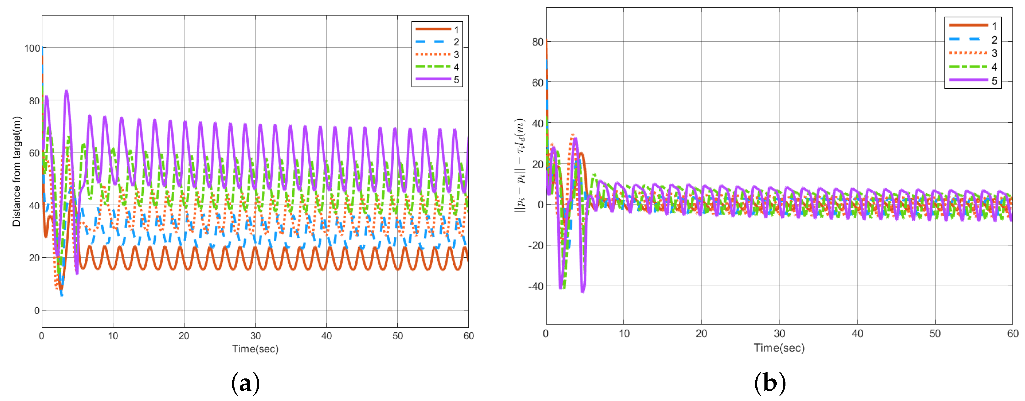
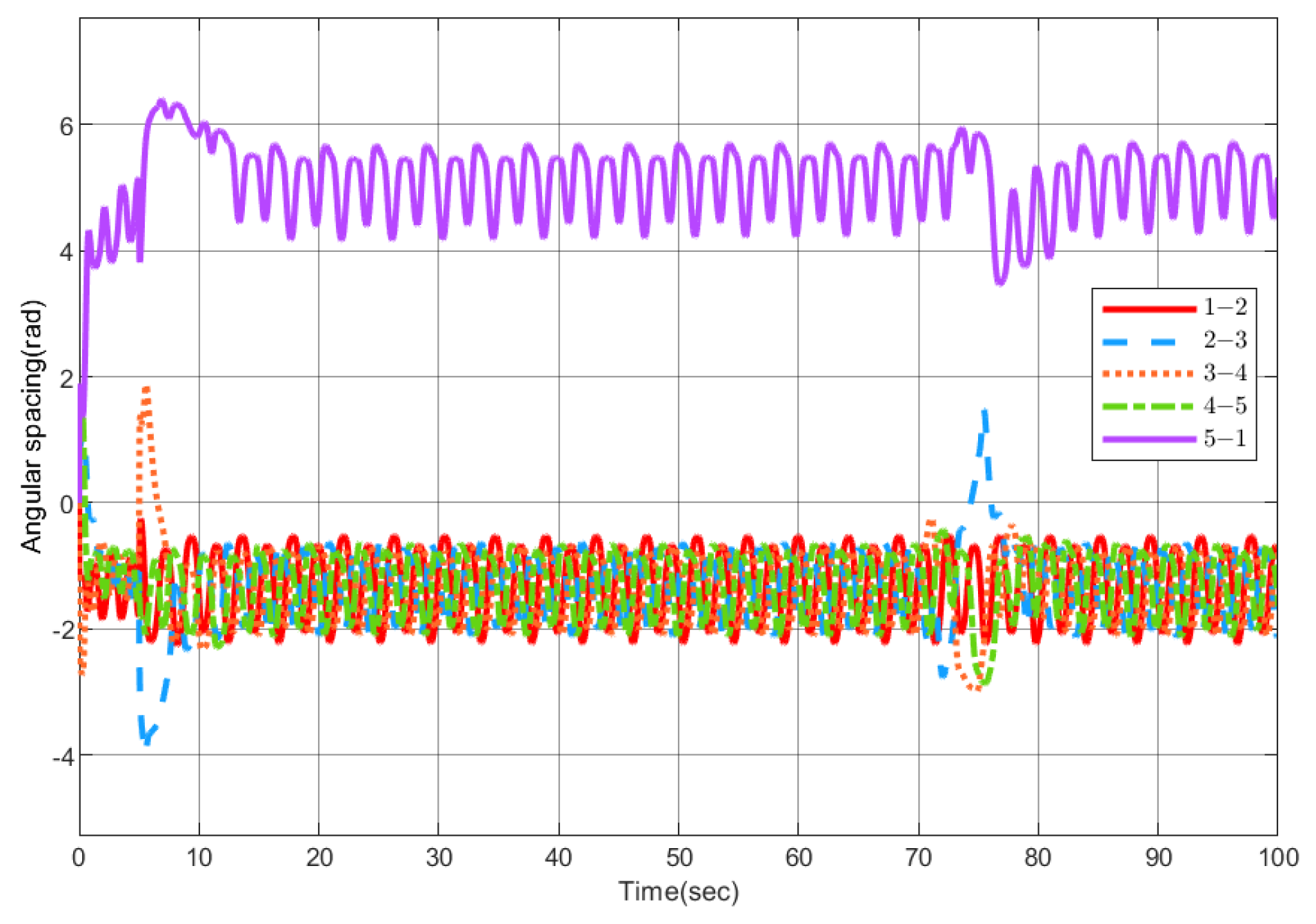
4.1. Case 1: Target Moves in a Straight Line

The speed of the moving target in three-dimensional space is selected as p t ˙ = [ 2 2 4 ] T .
First, the parameters of the estimator are selected, k = 1 , and the initial positions of the five UAVs are randomly generated. Figure 6 presents the simulation results of the convergence effect of the position estimator.
Next, when external interference is not considered, that is d i = [ 0 , 0 , 0 ] T , the parameters of the elliptical orbit are taken as a = 25 and b = 15, with τ i selected as τ i = [ 1 , 1.5 , 1.8 , , 2.3 , 2.8 ] .
Figure 7 shows the angular spacing between two adjacent UAVs, Figure 8 gives the circumnavigation control error, and Figure 8a shows distance between each UAV and the target, that is | | p i p t | | . Since the circumnavigation track is elliptical, the distance should change all the time. Figure 8b is | | p i p t | | τ i l d , that is, the error between the actual distance and estimated distance from the position of UAV to target. The three-dimensional simulation diagram of the UAVs circumnavigation is given in Figure 9.
Since the UAV is easily interfered with by external factors during the operation, the robustness of the control system is tested. When t = 70 s, the external interference of the third UAV is set to d 3 = [ 0 , 30 , 70 ] T . Figure 10 shows the change in the angular spacing between each UAV, and Figure 11 shows the circumnavigation control error, where Figure 11a is | | p i p t | | , and Figure 11b is | | p i p t | | τ i l d . It can be seen from the above pictures that when there is interference, the sliding mode control can quickly eliminate the influence of the interference and maintain the formation of the UAV group.

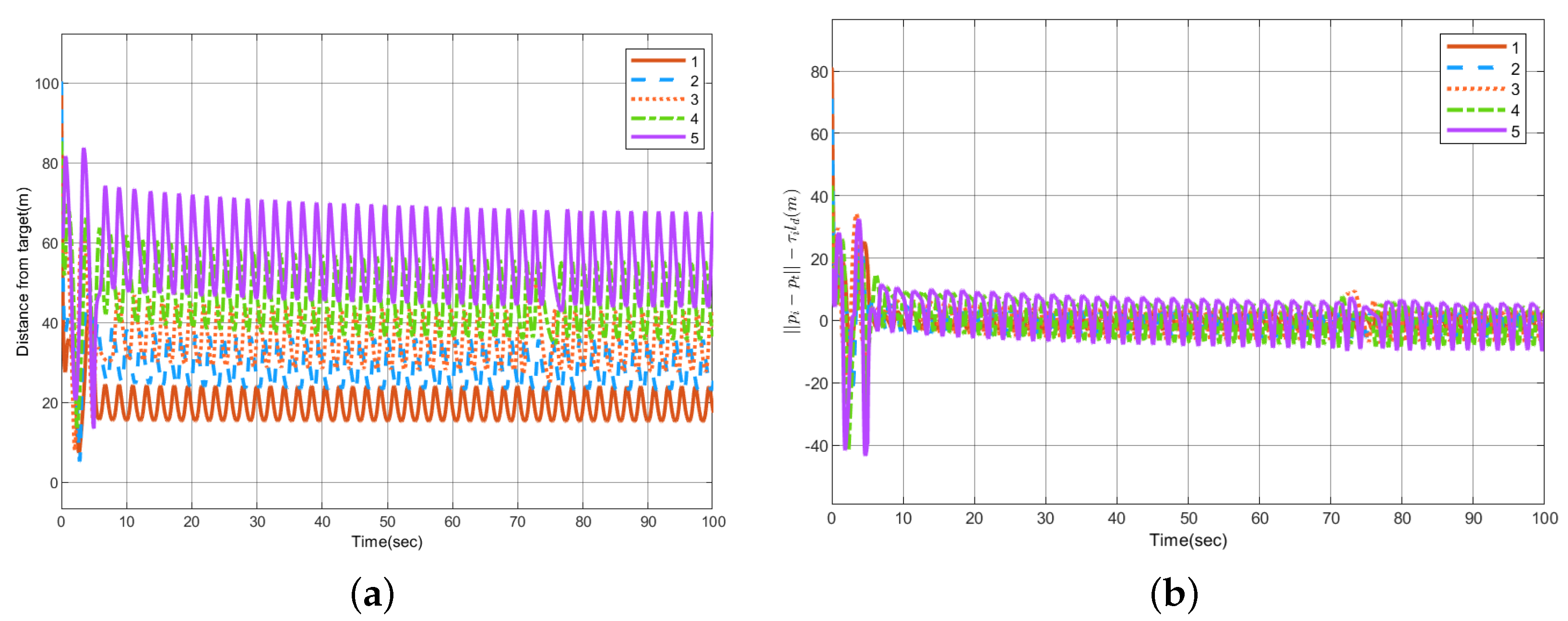
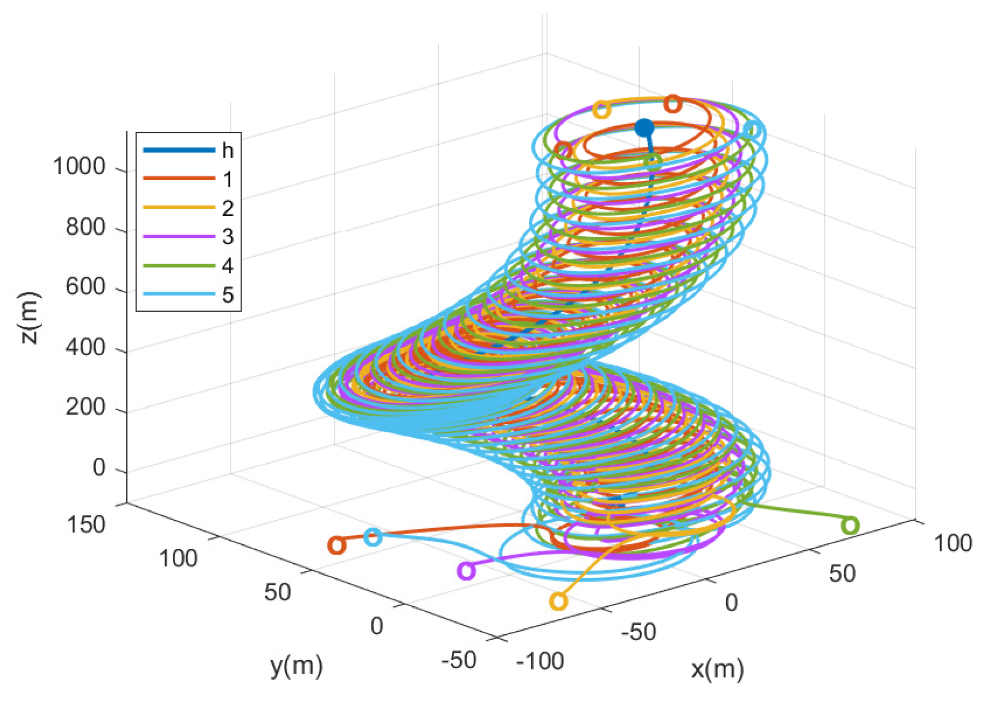
4.2. Case 2: Target Moves in a Curve

The speed of the moving target in three-dimensional space is selected as p ˙ t = [ 3 cos ( 0.5 t ) 3 sin ( 0.5 t ) t ] T .
The parameters of the estimator are selected, k = 1, and the initial positions of the five UAVs are randomly generated. Figure 12 presents the simulation results of the convergence effect of the position estimator.
When d i = [ 0 , 0 , 0 ] T , we take the parameters of the elliptical orbit as a = 30 and b = 20, with τ i selected as τ i = [ 1 , 1.2 , 1.4 , , 1.6 , 1.8 ] .
Figure 13 shows the angular spacing between two adjacent UAVs, Figure 14 gives the circumnavigation control error, and Figure 14a shows the distance between each UAV and the target, that is | | p i p t | | . Figure 14b is | | p i p t | | τ i l d . The three-dimensional simulation diagram of the UAVs circumnavigation is given in Figure 15.
The robustness of the system is verified again. When t = 70 s, the external interference of the fifth UAV is set to d 3 = [ 30 , 10 , 50 ] T . Figure 16 shows the change in the angular spacing between each UAV, and Figure 17 shows the circumnavigation control error, where Figure 17a is | | p i p t | | , and Figure 17b is | | p i p t | | τ i l d . The above experiments once again prove that the sliding mode control adopted in this paper has strong robustness.

5. Conclusions

In this paper, the problem of circumnavigation control in three-dimensional space is studied, the group of UAVs is made to circle the target in elliptical formation and with multiple orbits. The target is made to move with curvilinear variable speed, and UAVs estimate the position of the target only from the angle information. The error dynamic equation is constructed using the ideal relative velocity and the actual relative velocity, and the circumnavigation control is transformed into a velocity tracking problem. In order to improve the robustness of the system, sliding mode control is used to design the control law. Finally, the effectiveness of the proposed control law is proved by simulation, and disturbance is added to the simulation process to verify the robustness of sliding mode control.

Author Contributions

Conceptualization, Y.L. and Z.W.; methodology, Z.W.; software, Z.W.; validation, Y.L. and Z.W.; formal analysis, Z.W.; investigation, Z.W.; resources, Y.L.; data curation, Z.W.; writing—original draft preparation, Z.W.; writing—review and editing, Y.L.; visualization, Z.W.; supervision, Y.L.; project administration, Y.L.; funding acquisition, Y.L. All authors have read and agreed to the published version of the manuscript.

Funding

This research was funded by the National Natural Science Foundation of China (62173082), Shenyang Science & Technology Innovation Program for Young and Middle-aged Talents (RC210503), and the Liaoning Joint Fund of the National Natural Science Foundation of China (U1908217).

Institutional Review Board Statement

Not applicable.

Informed Consent Statement

Not applicable.

Data Availability Statement

Not applicable.

Conflicts of Interest

The authors declare no conflict of interest.

References

  1. Luo, Y.; Yu, X.; Yang, D.; Zhou, B. A survey of intelligent transmission line inspection based on unmanned aerial vehicle. Artif. Intell. Rev. 2022, 1–29. [Google Scholar] [CrossRef]
  2. Israr, A.; Ali, Z.A.; Alkhammash, E.H.; Jussila, J.J. Optimization Methods Applied to Motion Planning of Unmanned Aerial Vehicles: A Review. Drones 2022, 6, 126. [Google Scholar] [CrossRef]
  3. Ming, Z.; Huang, H. A 3d vision cone based method for collision free navigation of a quadcopter UAV among moving obstacles. Drones 2021, 5, 134. [Google Scholar] [CrossRef]
  4. Lan, Y.; Lin, Z.; Cao, M.; Yan, G. A distributed reconfigurable control law for escorting and patrolling missions using teams of unicycles. In Proceedings of the 49th IEEE Conference on Decision and Control, Atlanta, GA, USA, 15–17 December 2010; pp. 5456–5461. [Google Scholar]
  5. Zhang, Y.; Wen, Y.; Li, F.; Chen, Y. Distributed observer-based formation tracking control of multi-agent systems with multiple targets of unknown periodic inputs. Unmanned Syst. 2019, 7, 15–23. [Google Scholar] [CrossRef]
  6. Zhang, M.; Jia, J.; Mei, J. A composite system theory-based guidance law for cooperative target circumnavigation of UAVs. Aerosp. Sci. Technol. 2021, 118, 107034. [Google Scholar] [CrossRef]
  7. Le, W.; Xue, Z.; Chen, J.; Zhang, Z. Coverage Path Planning Based on the Optimization Strategy of Multiple Solar Powered Unmanned Aerial Vehicles. Drones 2022, 6, 203. [Google Scholar] [CrossRef]
  8. Yan, J.; Yu, Y.; Wang, X. Distance-Based Formation Control for Fixed-Wing UAVs with Input Constraints: A Low Gain Method. Drones 2022, 6, 159. [Google Scholar] [CrossRef]
  9. Leonard, N.E.; Paley, D.A.; Lekien, F.; Sepulchre, R.; Fratantoni, D.M.; Davis, R.E. Collective motion, sensor networks, and ocean sampling. Proc. IEEE 2007, 95, 48–74. [Google Scholar] [CrossRef] [Green Version]
  10. Kothari, M.; Sharma, R.; Postlethwaite, I.; Beard, R.W.; Pack, D. Cooperative target-capturing with incomplete target information. J. Intell. Robot. Syst. 2013, 72, 373–384. [Google Scholar] [CrossRef]
  11. Sepulchre, R.; Paley, D.A.; Leonard, N.E. Stabilization of planar collective motion: All-to-all communication. IEEE Trans. Autom. Control 2007, 52, 811–824. [Google Scholar] [CrossRef]
  12. Sepulchre, R.; Paley, D.A.; Leonard, N.E. Stabilization of planar collective motion with limited communication. IEEE Trans. Autom. Control 2008, 53, 706–719. [Google Scholar] [CrossRef] [Green Version]
  13. Marshall, J.A.; Broucke, M.E.; Francis, B.A. Formations of vehicles in cyclic pursuit. IEEE Trans. Autom. Control 2004, 49, 1963–1974. [Google Scholar] [CrossRef]
  14. Deghat, M.; Shames, I.; Anderson, B.D.; Yu, C. Localization and circumnavigation of a slowly moving target using bearing measurements. IEEE Trans. Autom. Control 2014, 59, 2182–2188. [Google Scholar] [CrossRef]
  15. Wang, J.; Ma, B.; Yan, K. Mobile Robot Circumnavigating an Unknown Target Using Only Range Rate Measurement. IEEE Trans. Circ. Syst. I Express Briefs 2021, 69, 2. [Google Scholar] [CrossRef]
  16. Greiff, M.; Deghat, M.; Sun, Z.; Robertsson, A. Target Localization and Circumnavigation with Integral Action in R2. IEEE Control Syst. Lett. 2021, 6, 1250–1255. [Google Scholar] [CrossRef]
  17. Summers, T.H.; Akella, M.R.; Mears, M.J. Coordinated standoff tracking of moving targets: Control laws and information architectures. J. Guid. Control Dyn. 2009, 32, 56–69. [Google Scholar] [CrossRef]
  18. Huo, M.; Duan, H.; Fan, Y. Pigeon-inspired circular formation control for multi-UAV system with limited target information. Guid. Navig. Control 2021, 1, 2150004. [Google Scholar] [CrossRef]
  19. Seyboth, G.S.; Wu, J.; Qin, J.; Yu, C.; Allgöwer, F. Collective circular motion of unicycle type vehicles with nonidentical constant velocities. IEEE Trans. Control Netw. Syst. 2014, 1, 167–176. [Google Scholar] [CrossRef]
  20. Hernandez, S.; Paley, D.A. Three-dimensional motion coordination in a spatiotemporal flowfield. IEEE Trans. Autom. Control 2010, 55, 2805–2810. [Google Scholar] [CrossRef]
  21. Kim, T.H.; Hara, S.; Hori, Y. Cooperative control of multi-agent dynamical systems in target-enclosing operations using cyclic pursuit strategy. Int. J. Control 2010, 83, 2040–2052. [Google Scholar] [CrossRef]
  22. Dong, F.; You, K.; Song, S. Target encirclement with any smooth pattern using range-based measurements. Automatica 2020, 116, 108932. [Google Scholar] [CrossRef] [Green Version]
  23. Cao, Y. UAV circumnavigating an unknown target under a GPS-denied environment with range-only measurements. Automatica 2015, 55, 150–158. [Google Scholar] [CrossRef] [Green Version]
  24. Shi, L.; Zheng, R.; Liu, M.; Zhang, S. Distributed circumnavigation control of autonomous underwater vehicles based on local information. Syst. Control Lett. 2021, 148, 104873. [Google Scholar] [CrossRef]
  25. Yu, X.; Liu, L. Cooperative control for moving-target circular formation of nonholonomic vehicles. IEEE Trans. Autom. Control 2016, 62, 3448–3454. [Google Scholar] [CrossRef]
  26. Sen, A.; Sahoo, S.R.; Kothari, M. Circumnavigation on multiple circles around a nonstationary target with desired angular spacing. IEEE Trans. Cybern. 2019, 51, 222–232. [Google Scholar] [CrossRef]
  27. Mehrabian, A.R.; Tafazoli, S.; Khorasani, K. Coordinated Attitude Control of Spacecraft Formation without Angular Velocity Feedback: A Decentralized Approach; Aerospace Research Central: Lawrence, KS, USA, 2009; p. 6289. [Google Scholar]
  28. Chen, Y.; Liang, J.; Miao, Z.; Wang, Y. Distributed Formation Control of Quadrotor UAVs Based on Rotation Matrices without Linear Velocity Feedback. Int. J. Control Autom. Syst. 2021, 19, 3464–3474. [Google Scholar] [CrossRef]
  29. Speck, C.; Bucci, D.J. Distributed uav swarm formation control via object-focused, multi-objective sarsa. In Proceedings of the 2018 Annual American Control Conference, Milwaukee, WI, USA, 27–29 June 2018; pp. 6596–6601. [Google Scholar]
  30. Qiao, L.; Zhang, W. Adaptive second-order fast nonsingular terminal sliding mode tracking control for fully actuated autonomous underwater vehicles. IEEE J. Ocean. Eng. 2018, 44, 363–385. [Google Scholar] [CrossRef]
  31. Bai, A.; Luo, Y.; Zhang, H.; Li, Z. L2-gain robust trajectory tracking control for quadrotor UAV with unknown disturbance. Asian J. Control 2021, 1–13. [Google Scholar] [CrossRef]
  32. Li, D.; Cao, K.; Kong, L.; Yu, H. Fully Distributed Cooperative Circumnavigation of Networked Unmanned Aerial Vehicles. IEEE/ASME Trans. Mechatron. 2021, 26, 709–718. [Google Scholar] [CrossRef]
Figure 1. Schematic diagram of three-dimensional space circumnavigation.
Drones 06 00296 g001
Figure 2. Top view of circumnavigation.
Drones 06 00296 g002
Figure 3. Multi-orbit circumnavigation.
Drones 06 00296 g003
Figure 4. Quadcopter UAV coordinate system.
Drones 06 00296 g004
Figure 5. Top view of the UAV i at time t.
Drones 06 00296 g005
Figure 6. Position estimator error convergence | | p ^ ti p t | | .
Drones 06 00296 g006
Figure 7. Angular spacing between adjacent UAVs.
Drones 06 00296 g007
Figure 8. Circumnavigation control error. (a) | | p i p t | | . (b) | | p i p t | | τ i l d .
Drones 06 00296 g008
Figure 9. Three−dimensional diagram of circumnavigation control.
Drones 06 00296 g009
Figure 10. Variation in angular separation between adjacent UAVs when interference occurs.
Drones 06 00296 g010
Figure 11. The circumnavigation control error when disturbance occurs. (a) | | p i p t | | . (b) | | p i p t | | τ i l d .
Drones 06 00296 g011
Figure 12. Position estimator error convergence | | p ^ ti p t | | .
Drones 06 00296 g012
Figure 13. Angular spacing between adjacent UAVs.
Drones 06 00296 g013
Figure 14. Circumnavigation control error. (a) | | p i p t | | . (b) | | p i p t | | τ i l d .
Drones 06 00296 g014
Figure 15. Three−dimensional diagram of circumnavigation control.
Drones 06 00296 g015
Figure 16. Variation in angular separation between adjacent UAVs when interference occurs.
Drones 06 00296 g016
Figure 17. The circumnavigation control error when disturbance occurs. (a) | | p i p t | | . (b) | | p i p t τ i l d | | .
Drones 06 00296 g017
Publisher’s Note: MDPI stays neutral with regard to jurisdictional claims in published maps and institutional affiliations.

