Article

Effects of Drainage Water Management in a Corn–Soy Rotation on Soil N2O and CH4 Fluxes

1
Appalachian Laboratory, University of Maryland Center for Environmental Science, Frostburg, MD 21532, USA
2
Department of Environmental Studies, University of North Carolina, Asheville, NC 28804, USA
3
Horn Point Laboratory, University of Maryland Center for Environmental Science, Cambridge, MD 21613, USA
4
Department of Environmental Science and Studies, Washington College, Chestertown, MD 21620, USA
5
Smithsonian Environmental Research Center, Edgewater, MD 21037, USA
6
University of Maryland Extension Caroline County, Denton, MD 21629, USA
*
Author to whom correspondence should be addressed.
Nitrogen 2022, 3(1), 128-148; https://doi.org/10.3390/nitrogen3010010
Submission received: 1 February 2022 / Revised: 4 March 2022 / Accepted: 9 March 2022 / Published: 17 March 2022

Abstract

:
Drainage water management (DWM), also known as controlled drainage, is a best management practice (BMP) deployed on drainage ditches with demonstrated success at reducing dissolved nitrogen export from agricultural fields. By slowing discharge from agricultural ditches, subsequent anaerobic soil conditions provide an environment for nitrate to be reduced via denitrification. Despite this success, incomplete denitrification might increase nitrous oxide (N2O) emissions and more reducing conditions might increase methanogenesis, resulting in increased methane (CH4) emissions. These two gases, N2O and CH4, are potent greenhouse gases (GHG) and N2O also depletes stratospheric ozone. This potential pollution swapping of nitrate reduction for GHG production could negatively impact the desirability of this BMP. We conducted three years of static chamber measurements of GHG emissions from the soil surface in farm plots with and without DWM in a corn–soybean rotation on the Delmarva Peninsula. We found that DWM raised the water table at the drainage ditch edge, but had no statistically significant effect on water-filled pore space in the field soil surface. Nor did we find a significant effect of DWM on GHG emissions. These findings are encouraging and suggest that, at least for this farm site, DWM can be used to remove nitrate without a significant tradeoff of increased GHG emissions.

1. Introduction

Excess agricultural nitrogen (N) and phosphorus (P) addition to the environment has been a long-term problem in the United States, contributing to algal blooms and eutrophication [1]. Within the Chesapeake Bay watershed agricultural production on the Delmarva peninsula accounted for ~90% of the nitrogen inputs [2,3,4], much of which is derived from synthetic nitrogen fertilizer [5]. Despite the need for nitrogen to increase crop yields, more than half of the N applied can be lost to the environment in a variety of pathways such as leaching and gas emissions [6,7]. Surface ditches and tile drains installed to remove water from wet fields act as conduits for export of dissolved nutrients. Drainage water management (DWM) is a best management practice (BMP) designed to slow this movement and thereby reduce reactive N loss from agricultural fields that have drainage ditches [8,9].
Drainage water management (DWM) functions by placing drainage control structures (DCS) at the end of drainage ditches with the goal of slowing water discharge and raising water levels in ditches. By keeping water in the field for longer, the water table upstream of the ditch rises, creating more widespread anaerobic soil conditions [10]. When N, as nitrate, is exposed to more reducing conditions microbially driven denitrification is more likely [11,12]. Some studies have demonstrated that DWM has been effective at reducing nitrate loading into downstream waters [13,14,15], including preliminary results from the farm of present study [16]. However, incomplete denitrification can result in nitrous oxide (N2O) production, a potent greenhouse gas (GHG) and a reactant in stratospheric ozone destruction [17,18]. In addition, nitrification has also been documented to produce N2O as a byproduct [11]. Agricultural soil management, driven by anthropogenic nitrogen inputs, is responsible for 75% of the total N2O emissions in the US and 45% of total N2O emissions in North America [19,20]. In addition to N2O, reducing conditions can also create higher methane (CH4) emissions via methanogenesis [21]. Methane is the second most important GHG, with potency 25-fold greater than CO2 in a 100 year time frame [22].
Broadly, soil N2O fluxes are controlled primarily by inorganic-N content, carbon availability, soil moisture, microbial community abundances, soil temperature, soil pH, and soil texture [11,12]. Fertilizer N can be rapidly converted to nitrate, through nitrification, and nitrate can then become substrate for denitrification. Both nitrification and denitrification can contribute to large N2O emission spikes [23], especially when high soil nitrate concentrations co-occur with high soil moisture conditions [24,25]. The combination of high N input with DWM that retains water in the field could result in lower hydrologic losses of N as nitrate through the ditch but with the tradeoff of higher losses of N2O.
Previous work examining the impact of water table changes and DWM on GHG emissions in agriculture fields has yielded contradictory results. Some studies found that undrained fields had higher N2O emissions than drained fields [26,27,28,29] while other studies found that there was no difference in N2O emissions between drained and undrained fields [30,31,32,33]. For CH4, one study [26] found higher emissions in undrained fields while others found no drainage effect on CH4 emissions [30,31,32]. Some of these studies did not directly evaluate DWM manipulations, creating higher and lower water tables at specific times of the year, rather they explored drainage impact in general [26,27,32], or drainage impact with subsurface irrigation [29,31]. The variability in conclusions and paucity of direct assessments of DWM mean that further research is needed to understand the impacts of this particular BMP on the potential for increased GHGs. Here, we compare measured soil emissions of N2O and CH4 in corn and soybean fields with controlled drainage (DWM) and free drainage (non-DWM) at a farm in eastern Maryland, on the Delmarva Peninsula. We hypothesized that DWM would increase soil GHG emissions.

2. Materials and Methods

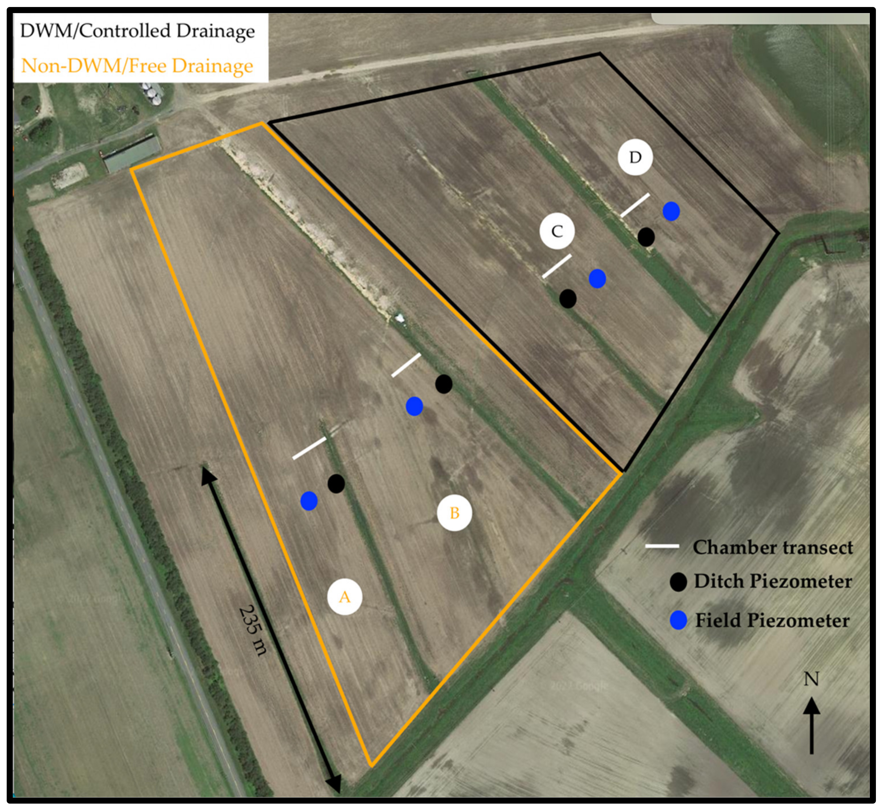
2.1. Study Site Location

The research site was located on a private farm within the Choptank watershed on the coastal plain of the Delmarva Peninsula on the Eastern Shore of Maryland (Figure 1, N 39.11973, W 75.8069). Historically a wet landscape, the land was made arable by installing drainage ditches. Harvested crops mostly contribute feed to nearby concentrated poultry production. Precipitation averages 110 cm per year. This study site is an operational farm with a collaborating farmer willing to accommodate our research needs while working within the timing of standard agricultural management. A DWM system was already in place and a direct evaluation of that system was possible in a relatively small area. The ditches split the site into four similarly sized fields ranging from 3 to 6 hectares each, with an average length of 220 m. The dominant soil type is a Fallsington series on 0–2 percent slopes classified as fine-loamy, mixed, active, mesic Typic Endoaquults.

2.2. Farm Management

The crop management plan was a no-till, corn–soybean rotation with a winter radish cover crop. The typical growing season ranged from April to October. Approximately 213 kg ha−1 of synthetic urea-ammonium nitrate (UAN) was applied during corn years and no N fertilizer was applied during soybean years. Approximately 22 kgN ha−1 was knifed-in during corn planting, and the other 191 kgN ha−1 was broadcast-applied in late May or early June. During corn planting, the fields received a sulfur addition of 15 kgS ha−1. Liquid or dry potash was applied during corn and soybean years. Herbicide was applied prior to or soon after planting and sometimes in June to suppress undesired vegetative growth. Prior to harvest, daikon radish seed was applied by air to serve as the winter cover crop. Manure and lime were applied every 5 years, which did not occur during this project’s duration. The site had pivot irrigation that was used to supplement natural precipitation events in the summer months. All the research fields had the same crop rotation schedule, N fertilization rate, and irrigation rate from 2017 to 2019.

2.3. DWM Management

The DWM strategy consisted of inserting and removing boards within the drainage control structures (DCS) to slow the ditch discharge while accommodating standard farm practices (Figure S1). For farm activities such as planting, N fertilization, and harvest, the DCS boards were removed and fields were drained to create a drier condition for equipment use. This management timeline was dependent on precipitation events, groundwater levels, and evapotranspiration; therefore the strategy was modified to adapt to changing environmental conditions. We refer to the time period when the boards were in place in the DWM DCS as “active” and the period when they were removed from the DWM DCS as “inactive”.

2.4. Experimental Design

Figure 1 shows a site map depicting the static chamber transect locations and borders of study plots. Non-DWM, or free drainage, was implemented on two fields (A and B) and controlled drainage, or DWM, implemented in the other two fields (C and D). In each field the soil chamber sampling design consisted of a transect of eight chambers installed perpendicular to the ditch. Each transect was approximately 12 m in length and the soil chamber collars were equally spaced. The replicate plots were adjacent to each other in order to increase the horizontal fetch of micrometeorological measurements of a companion part of this study that will be reported elsewhere.
Soil and soil gas flux measurements were taken approximately monthly, depending on climatic conditions, but more temporally intensive sampling was done around planting, irrigation, N fertilization, and harvest to better characterize trace gas dynamics during those periods. Because preliminary studies showed some diel variation (Figure S2), the order of chamber sampling was randomized to ensure that the same field was not measured at the same time of day during every sampling date, thus minimizing potential sampling biases due to diel variation. Fluxes were sampled starting at approximately 8:00 EST and extended until approximately 17:00 EST.
Two slotted PVC (5 cm diameter) piezometers, used to measured groundwater levels, were installed approximately 1.5–2 m deep in the four research fields. One piezometer was installed within 1 m of the perimeter of the ditch while another was placed in the field 15 m perpendicular to the ditch piezometer (Figure 1). The piezometers were located within 15 m of the chamber transect. Solinst water level data loggers were placed in each piezometer which recorded pressure and temperature every 30 min. The pressure was then converted to depth of water below the surface by subtracting barometric pressure recorded separately by a Solinst barologger. Thirty-minute water depths were aggregated to daily mean for this analysis.
There were four primary controls on the statistical power of this experimental design: (1) plot replication, (2) number of chamber measurements in each plot, (3) number of days of sampling over three years and (4) number of gas concentration measurements used to calculate each flux. This experimental design was limited to two replicate plots per treatment because four was the maximum number of flux towers that could be established in the companion micrometeorological study. The within-plot statistical power of this study was provided by eight chambers per field, which was needed for measurements known to have high spatial variability, as is the case with N2O and CH4 [34]. This study had excellent statistical strength in the number of gas concentration measurements per flux calculation, as there was a single chamber headspace concentration recorded every second (1 Hz), which increased the flux estimation accuracy, lowered the flux detection limit, reduced the time needed for each flux measurement, and afforded improved statistical analysis [35].

2.5. Flux Measurements

A Picarro G2308 cavity ringdown spectrometer and a static soil chamber system were used to measure N2O and CH4 soil gas fluxes. The instrument specifications state that the raw precision (1σ) of the instrument was <25 ppb + 0.05% of the reading for N2O and <10 ppb + 0.05% of the reading for CH4. The chambers consisted of a PVC chamber top with a curled vent, 12 cm length and 1 mm ID, and a matching PVC chamber collar. The chamber was approximately 25 cm in diameter. The chamber collar height was 5 cm and was inserted 3–4 cm into the soil. The chamber top height was 2.5 cm and had a rubber gasket around the perimeter to ensure a tight fit onto the collar. The approximate total volume of the chamber, dependent on insertion depth into the soil, was 4 L. The flux measurement system used a recirculation technique through inlet and outlet tubing connected to the instrument, air pump, and the chamber top. Twenty-meter lengths of 6 mm OD polyethylene tubing connected the gas analyzer to the chamber top. Given the average flow rate of the pump (~230 mL min−1), the tubing diameter, and length, it took approximately 45 s for gas to reach the analyzer from the chamber. Because of the high frequency (1 Hz) of reporting concentration by the instrument and its high sensitivity to change in concentration, the chamber top was left on each collar for only ~5 min, which was sufficient time to detect a non-zero slope of increasing or decreasing headspace concentrations, while minimizing a potential chamber artifact of altering the concentration gradient between soil and headspace gas. The slope was used to calculate a flux using Equation (1)
F lux   mol   m 2   min 1   = dConc dt P V A R T
where dConc/dt = slope (μL L−1 min−1), P = air pressure (atm), R = gas law constant (L atm mol−1 K−1), T = air temperature (K), V = chamber volume (L), and A = chamber area (m2). Flux units of μmol m−2 min−1 were used for statistical analyses, but when flux interpolations and annual estimates were conducted, the flux units were converted to μg N2O-N m−2 min−1.

2.6. Soil Chemical and Physical Characteristics

Volumetric water content (VWC) of the soil was measured using a manual Decagon 5TM soil moisture probe. The probe was inserted vertically into the soil surface to a depth of 5 cm. At each chamber location (n = 32), three VWC measurements were taken outside the chamber area, and the mean calculated. The probe calibration was checked in the laboratory prior to field usage and the VWC was obtained using the Topp equation [36].
Soil samples used for gravimetric soil moisture, nitrate and ammonium concentration analyses were taken using a 2.2 cm diameter soil push probe during each gas flux measurement. At each chamber (n = 32) three, 5 cm deep soil plugs surrounding the chamber were collected and placed together into a labeled bag. The bag was placed in a refrigerated cooler, transported back to the laboratory and processed within 48 h. At the lab, the soil within each bag was homogenized and sieved using a 10 mesh (2 mm) pan. Six grams of the field-moist sieved soil were extracted in 30 mL of 2M potassium chloride (KCL), placed on an oscillating shaker table for at least 2 h, and vacuum filtered through a Whatman No. 42 filter paper. Extracts were then analyzed for nitrate, nitrite, and ammonium concentration using flow injection analysis Lachat autoanalyzer [37]. If samples were not processed in the analyzer within 12 h, they were stored at 4 °C until analysis within 30 days of soil collection. Soil push probe samples from five sampling dates selected over the three-year study were also analyzed for total soil carbon and total soil nitrogen using a Carlo Erba NC2500 elemental analyzer.
The surface bulk density of the soil was measured using a 5 cm length, 5 cm diameter PVC core. Air-dried soil was sieved with 10 mesh (2 mm) pan and weighed. The bulk density was calculated as the <2 mm air-dried mass divided by the volume. Two bulk density surface cores were taken in each field for two years of this study and averaged by field and year. Surface bulk density measurements were used to convert VWC to water-filled pore space (WFPS) by calculating the total porosity assuming a particle density of 2.65 g cm−3 [38]. Soil texture was assessed twice using hand augered soil samples at 10 cm intervals to an approximate depth of 1 m, twice, in each field. The soils were sieved using a 10 mesh (2 mm diameter) pan, air-dried for at least 72 h, and measured for soil texture using the hydrometer method [39].

2.7. Non-Parametric DWM Impact Model

The purpose of this model was to determine if the dependent variables (gas fluxes, piezometer depth, soil moisture) were impacted by DWM. Because of non-normality and heteroskedasticity of the dependent variable data, a non-parametric Wilcoxon test was used. The piezometer water depth, soil moisture and fluxes were assessed separately as dependent variables of interest. The independent variables were treatment (DWM/controlled drainage; versus non-DWM/free drainage) and board period (active—DCS boards inserted in the DWM plots; versus inactive—DCS boards removed for the farmer’s management activities). A pairwise post hoc test was performed to estimate p-values assessing the difference between board periods under both treatment conditions.

2.8. Mixed-Effects Model

A generalized linear mixed-effects model (GLMER) in R program was used to assess the impact of treatment and other predictor variables on N2O and CH4 fluxes. Both N2O and CH4 fluxes were non-normal and right skewed, so a natural log transformation was applied. A small positive offset was added to make all values positive before log transformation [40]. A gamma log link distribution was applied in the GLMER model [41].
For N2O, the independent variables of treatment, fertilization period, year, and board period were categorical variables assessed as fixed effects. Chamber location (1–8, with 1 being closest to the ditch and 8 being furthest) was a continuous variable serving as a measure of distance from ditch edge. After distance from the ditch was found to not be a significant fixed effect (p > 0.05), chamber number was then considered a random effect. Sampling dates were considered part of the fertilization period if they occurred within a window of 4 weeks after a fertilization event. Several studies have shown a peak of N2O emissions within days of fertilization, followed by a gradual decline over 2–4 weeks [24,42,43]. Board period was the same categorical variable as described in Section 2.7. Interaction effects between all fixed effects were also evaluated. Final models were selected based on the lowest AIC value of multiple fixed effect combinations and interactions. An estimated marginal means post hoc test was conducted when p-values of main effects were less than 0.05. Model residuals were visually analyzed for normality and heteroskedasticity.
For CH4, the independent variables of treatment, seasonal period, board period, and year were categorical variables assessed as fixed effects. Chamber location (1–8, with 1 being closest to the ditch and 8 being furthest) was initially tested as a continuous variable serving as a measure of distance from ditch edge but was not significant (p > 0.05), therefore distance was considered a random effect. Seasonal period was assigned a value based on inclusion within the data range of 1 April–30 June. These dates were selected because they corresponded to the beginning of the warmer spring season with wet soil conditions, prior to drier summer months. The final model was selected based on the lowest AIC value of multiple fixed effect combinations and interactions. An estimated marginal means post hoc test was conducted when p-values of main effects were less than 0.05. Model residuals were visually analyzed for normality and heteroskedasticity.

2.9. Regression Statistics

To examine how environmental variables controlled N2O emissions, a stepwise linear regression was created using soil temperature, soil water-filled pore space (WFPS), and nitrate concentration as the predictor variables for N2O emissions. The data were unaggregated, so each chamber flux measurement was an observation, for a total of 536 measurements with a complete suite of data for all dependent and independent variables. All data were tested for normality using the Shapiro–Wilk normality test and were log-transformed. For WFPS, a quadratic term was added to the model to account for an expected non-linear response [11]. The stepwise regression created multiple models with different combinations of predictor variables. The model with the lowest AIC was selected. Homoscedasticity and normality were assessed in the final model residuals.

2.10. Annual Flux Calculations

2.10.1. Seasonally-Based Flux Interpolation

To estimate an annual N2O gas flux, each year was divided into 3–4 periods, detailed in Table S1, bounded by farm management events and observed seasonal impacts of patterns of measured fluxes. For periods in which no visually obvious N2O spikes occurred, an arithmetic mean was taken of all the flux measurements within that time period and multiplied by the number of days within that period. For periods in which a spike of N2O flux was observed followed by a sustained drop in flux values, usually within days or weeks after N fertilization in corn years or shortly after temperature and moisture increase in the soybean year, a decay curve and function were fitted to the data for the duration of those observations (Figure S3). Daily fluxes were then summed to obtain a total period value. The emission values in each period (both arithmetically derived and decay curve derived) were summed to obtain an annual flux measurement. There were 3–4 periods per year with 2 to 5 flux measurements per period. This procedure was repeated to calculate an annual flux for each chamber. The chamber annual fluxes were averaged by treatment and a 95% confidence interval (CI) was calculated, representing spatial flux variability.
For CH4, each year was divided into 3 periods bounded by seasonal impacts on measured fluxes (Table S2). A mean flux was calculated for each period, multiplied by the number of days within that period, and period fluxes were summed to obtain an annual CH4 flux. This procedure was repeated for each chamber and the chambers were averaged by treatment to obtain a 95% CI representing the spatial variation within the treatment.

2.10.2. Mixed-Effects Model Extrapolation

For an independent check on the interpolation method, annual CH4 and N2O fluxes were also calculated by extrapolating the mean flux values reported in the mixed-effects model results for each year. This more simplistic approach did not account specifically for observed spikes in gas fluxes but represented the spatial and temporal variation accounted for in the mixed-effects model. An error term for each annual estimate was calculated based on the standard errors of the estimates of the mixed-effects model output.

2.10.3. Regression Model N2O Flux Interpolation

A regression-based model was used to obtain another independent annual N2O flux estimate using environmental variables of soil moisture, soil nitrate, and soil temperature. Linear interpolations were made between each of the measured data points for these environmental drivers. The interpolated daily variable values were applied to a stepwise linear regression equation. Predicted hourly N2O fluxes were summed to an annual flux. This was done for each chamber (n = 32) and an average and standard error were calculated by treatment.

3. Results

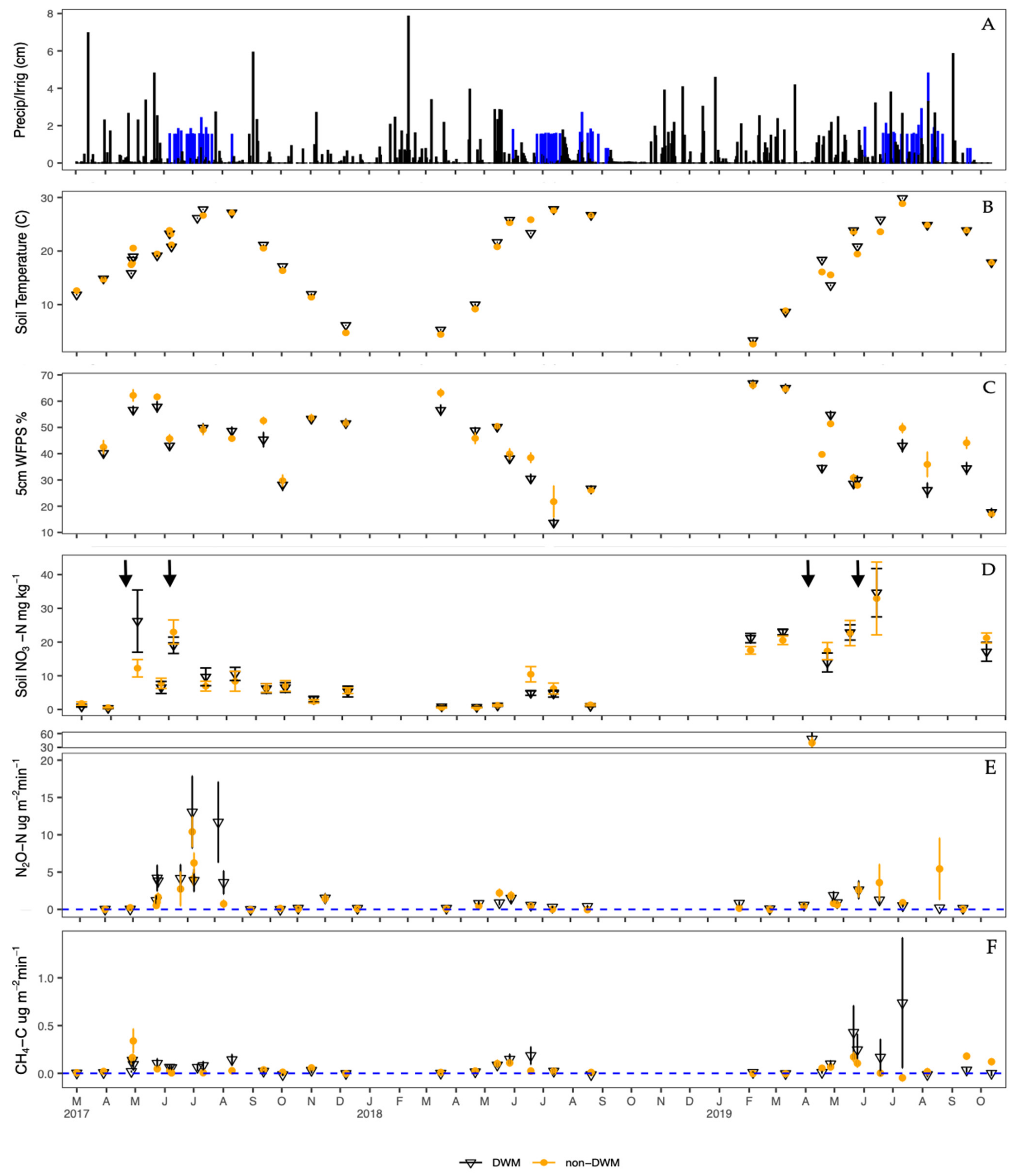
3.1. Environmental Variables

The following section describes the climatic and soil variables measured to complement the flux measurements (Figure 2).

3.1.1. Precipitation and Air Temperature

Daily precipitation and irrigation amounts were recorded over the course of this study (Figure 2A). The highest daily rainfall was 7.84 cm in February 2018. Seasonally averaged over three study years (2017–2019), March–May had the highest average rainfall with 31.8 ± 1 cm, followed by December–February with 26.4 ± 3.6 cm, June–August with 19.1 ± 8.6 cm, and September–November with 9.0 ± 1.9 cm. The daily average air temperature over three years was 14.1 °C and ranged from −13.0 to 30.1 °C (data not shown).

3.1.2. Soil Temperature and Moisture

Soil temperature and moisture at 5 cm depth were measured at the same frequencies as chamber fluxes. Soil temperature ranged from 2.1 to 29.1 °C and followed expected seasonality trends (Figure 2B). The measured mean percent water-filled pore space (%WFPS) by treatment ranged from 13% to 67% over the study period (Figure 2C). The highest recorded soil moisture contents occurred in the winter (December–February) and spring (March–May), and the lowest soil moisture contents occurred during the summer (June–August) and fall (September–November). There was a particularly dry period in July 2018, when the lowest soil moisture content of this study was recorded. Statistical analysis of WFPS can be found in results Section 3.4.

3.1.3. Soil Extractable Nitrogen

The soil extractable nitrate in the top 5 cm, measured at each chamber sampling, ranged from 0.38 to 34.6 mg N kg−1 (Figure 2D). In April 2017 and 2019, 22 kg N ha−1 as UAN fertilizer were applied during planting and in June 2017 and 2019 200 kg N ha−1 as UAN were applied, as indicated by arrows in Figure 2. In general, there was a positive association between N fertilization and soil nitrogen concentration. Soil nitrate values increased soon after application of N fertilizer in April and June of 2017 and 2019. After this period, the soil nitrate concentrations decreased throughout the remainder of the year. In the 2018 soybean crop, the soil nitrate values rose in the spring but did not reach concentrations as high as the years with N fertilization. For soil extractable ammonium values, the concentrations remained below 10 mg N kg−1 during the study period, except one measurement in June 2018 (data not shown). Ammonium values were more variable than nitrate and higher during summer than during winter.

3.1.4. Soil Texture and Bulk Density
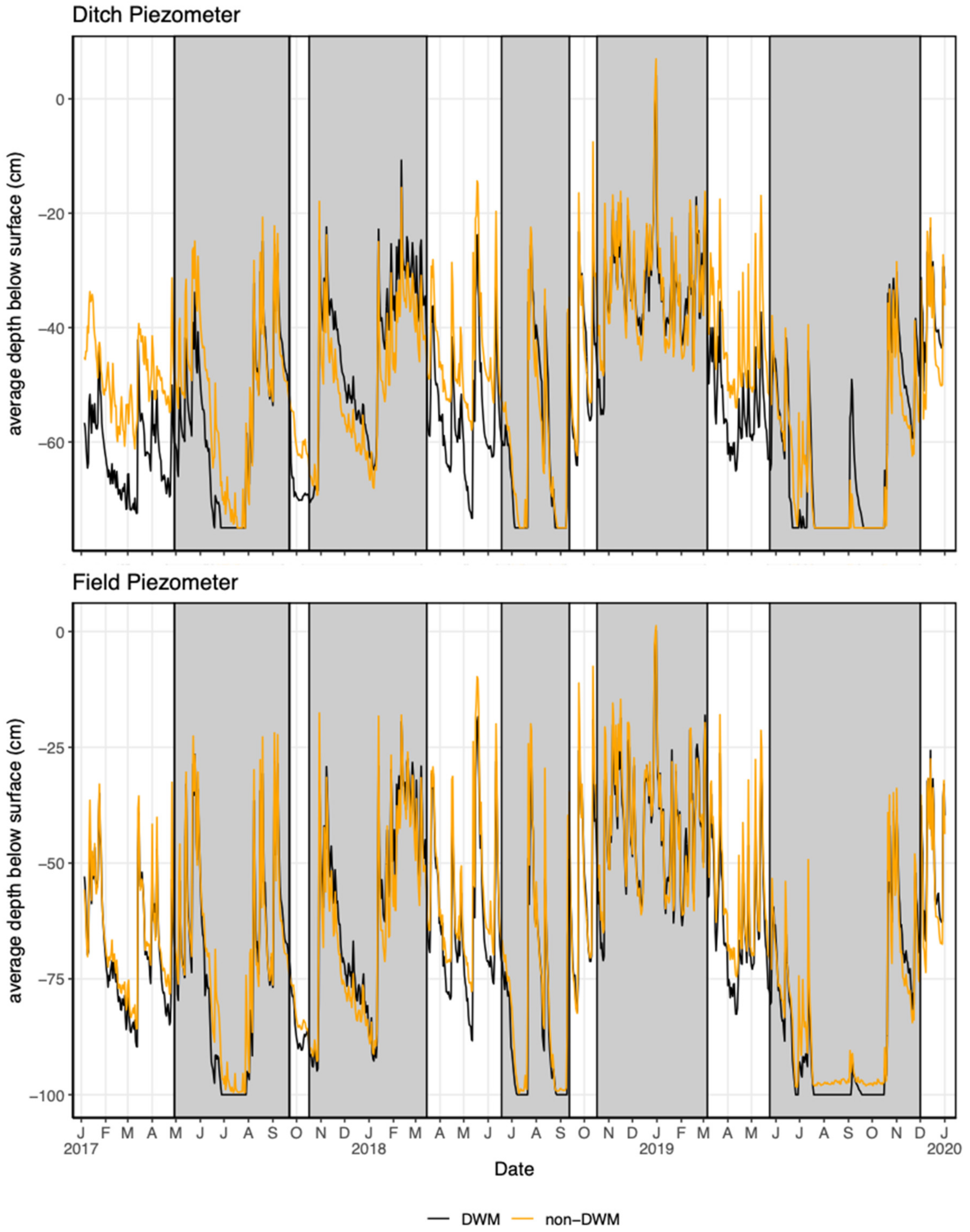
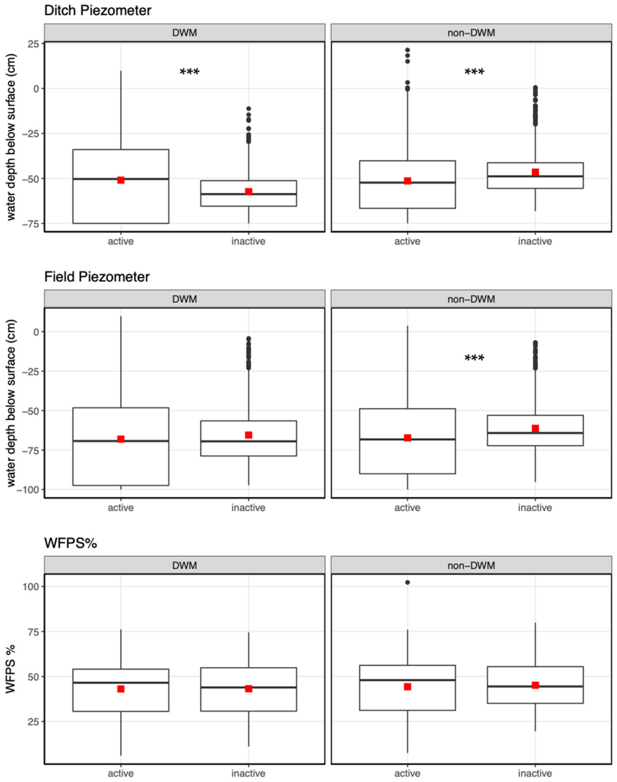
Soil texture varied spatially within and between the four fields. Augered soil cores in field C had higher clay and silt content compared to fields A, B, and D at depths ranging from 20 to 60 cm (Figure S4 and Table S3). The 5 cm surface bulk density values, %C, and %N also varied by field, with higher %C and %N values associated with higher clay content (Table S4).

3.2. Piezometers

The daily mean piezometer water depth was aggregated by treatment and piezometer location during the inactive and active DWM DCS board periods (Figure 3). In the ditch piezometers, in the DCS inactive (unshaded) periods, the DWM depth values were generally deeper than the non-DWM plot values, indicating spatial heterogeneity across the field. During the DCS active (shaded) periods, however, the lines on Figure 3 tend to converge, indicating that the DCS active installation of boards in the DWM plots increased the ditch piezometer water levels. In the field piezometers, the effect of board placement is less clear. The statistical evaluation of these piezometer data were combined analysis of WFPS data and are found in Section 3.4.

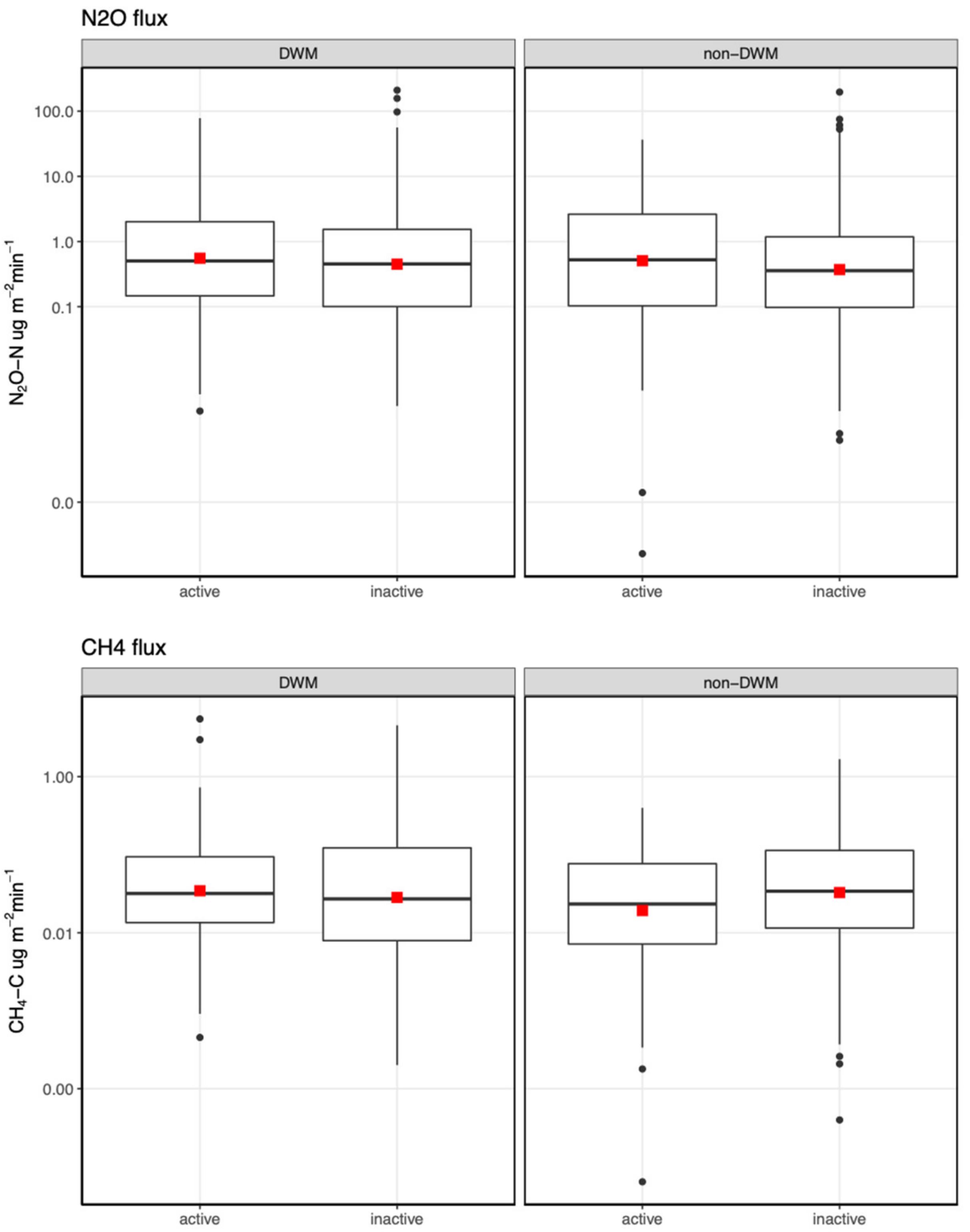
3.3. Chamber Flux Summary

From 2017 to 2019, 959 chamber flux measurements were taken. Most fluxes were small and the data had right-skewed distribution. When calculating the fluxes using the change in slope over time, assessed by linear regression, 96% of the methane slopes were significantly different from zero (p < 0.05) and of those 21% were negative, indicating CH4 consumption events. For N2O, 85% of the N2O slopes were significantly different from zero (p < 0.05) and 15% of those were negative. Because of the data skew, a log transformation was applied for parametric statistical analyses. An analysis of the minimum detectable flux (MDF) is provided in the Supplementary Materials (Table S5).
Figure 2E shows the N2O-N flux data, averaged by treatment. The highest emissions occurred after N fertilization events (planting or broadcast) in the April–July period of 2017 and 2019, marked by arrows. In 2017, the larger N2O peak occurred during the second fertilization and in 2019, after the first fertilization. The large response to the first fertilization in April 2019 N application may have resulted from co-occurrence of a precipitation event the day following application. Soil N2O consumption events occurred at various times throughout this study at the individual chamber scale, but never as the average flux from all chambers at the field scale. This indicates small scale flux variability within a field, but not net negative fluxes at the field scale.
For CH4, the highest CH4 emissions occurred in the spring period (April–June; Figure 2F). Several individual chambers showed net consumption of atmospheric CH4, but only rarely did this translate to net consumption as the mean at the field or treatment scale.

3.4. Non-Parametric DWM Model for Effects on Piezometers, WFPS, and Gas Fluxes

The non-parametric statistical analysis results for dependent variables of ditch piezometer, field piezometer, and surface WFPS showed differences in the interaction of treatment and board period (Figure 4). For the ditch piezometers, the mean water depth below ground was significantly deeper during the inactive DCS period than the active DCS period in the non-DWM sites. However, this trend was reversed in the DWM sites, with a higher mean water depth in the active DCS period compared to the inactive DCS period, indicating that the additional boards in the DWM sites raised the water table near the ditch, even during the dry summer. The field piezometer water levels showed the same trends as the ditch piezometers, except that the mean water level between active and inactive DCS periods was not significantly different in the DWM condition, indicating that the additional boards in the DWM sites had less of an effect on the water table in the mid-field, approximately 15 m from the ditch. The DWM only raised the water table in the mid-field piezometers to the same level as the non-DWM plots in the active DCS season, but did not exceed it, as was the case for the ditch piezometers (Figure 4). The WFPS showed no significant differences by treatment or board period, indicating the DWM did not affect near surface moisture content. The same non-parametric analysis for gas fluxes showed no significant differences by treatment or board period, indicating the DWM did not impact the soil gas fluxes in the fields (Figure 5).

3.5. Mixed-Effects Model Results for N2O and CH4 Fluxes

The purpose of the mixed-effects model was to assess the impact of the DWM treatment and other dependent variables. For N2O fluxes, the effects of the post-N fertilization period, year, chamber location, and interactions were assessed using two sub-models. In the first sub-model, the N fertilization effect was evaluated using only 2017 and 2019 data (corn years) because 2018 data (soybean year) did not have a N fertilization period. In the second sub-model the effects of treatment and year were assessed using all years’ data, but N fertilization variable was not included. The mixed model results (Table 1) show that DWM did not significantly affect N2O fluxes, which is consistent with the non-parametric model results (Figure 4 and Figure 5). Year had a significant effect on N2O fluxes, as the fertilized corn years of 2017 and 2019 had higher N2O fluxes compared to the unfertilized soybean year of 2018. The post hoc test showed that the N2O fluxes in 2017 and 2019 were not significantly different. Using the sub-model with only data from N fertilization years, the post-N fertilization period had significantly higher N2O fluxes than the non-fertilization period (Table 2). No interaction effects between independent variables were significant.
For CH4, DWM treatment, year and season were tested. CH4 emissions did not have significant differences based on year or treatment (Table 1). The spring seasonal period had higher CH4 emissions compared to the non-spring periods (Table 2).

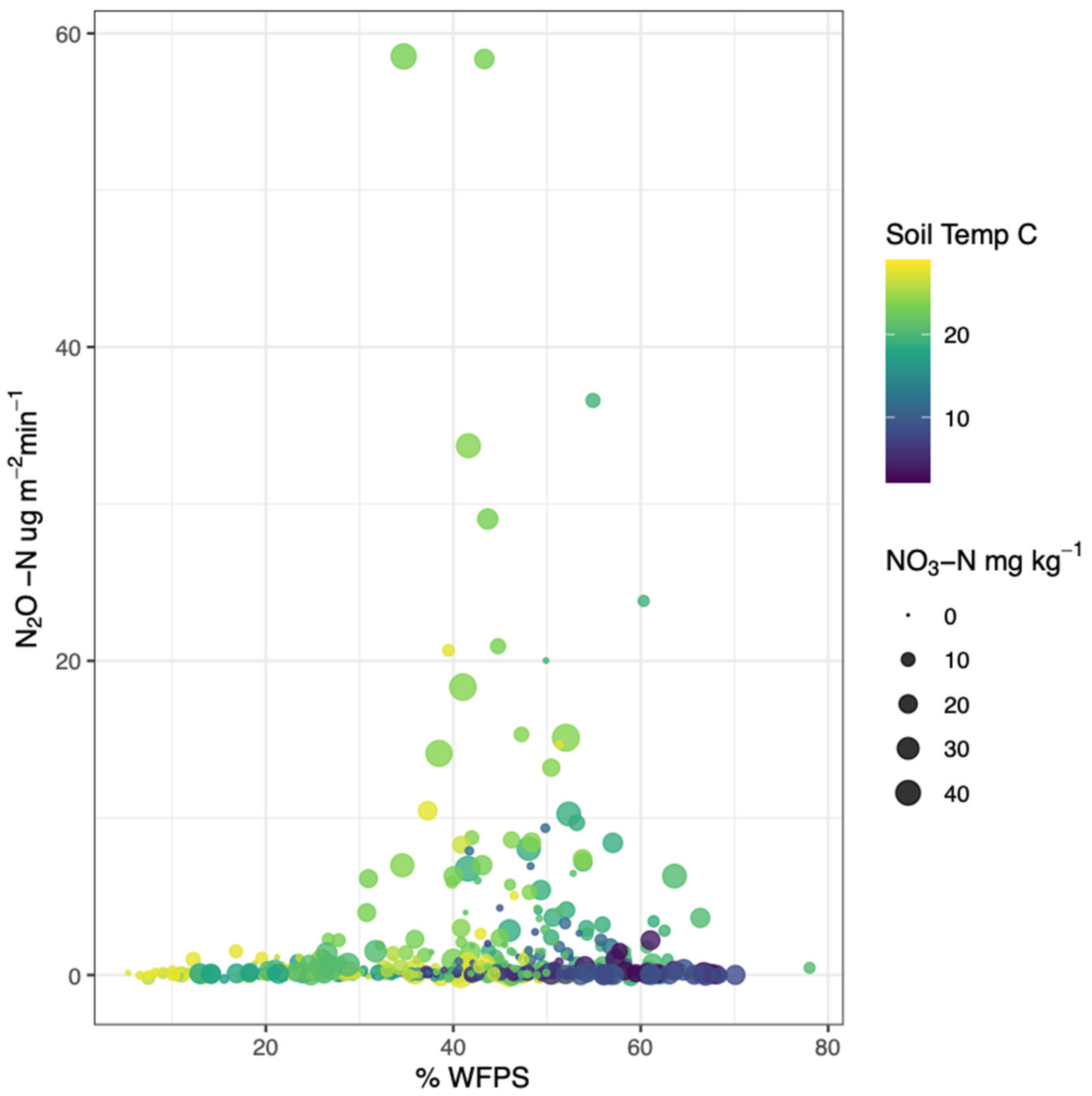
3.6. N2O Multiple Regression

There was a weak positive linear relationship (r2 = 0.12, p < 0.001, Figure S5) between soil nitrate and N2O fluxes. The largest N2O fluxes occurred when soil nitrate concentrations were high, but some large N2O fluxes also occurred at lower soil nitrate concentrations. For soil temperature, the higher N2O emissions occurred above 12 °C, although it should be noted that N fertilization events also only occurred during periods above this temperature. For WFPS, the highest N2O emission events occurred at intermediate WFPS values, but not all N2O flux events between those WPFS values resulted in high emissions. The highest N2O emissions typically occurred when the following combination of conditions existed: the soil temperature was above 12 °C, nitrate concentration was at least 10 mg N kg−1, and WFPS was between 35% and 60% (Figure 6).
The stepwise linear regression yielded the lowest AIC when the model included all terms, including a quadratic term for WFPS. The most important predictor variable was soil nitrate followed by soil temperature, and WFPS. The full model (Equation (2)) and each predictor variable were significant (p < 0.001), and the full model yielded an r2 value of 0.23 (Table S6).
ln   N 2 O + 1 = 0.029   NO 3 N + 0.021 soil   temp + 0.056 WFPS 0.001 WFPS 2 1.37
where N2O is N2O flux (μg N2O-N m−2 min−1), NO3-N is concentration of nitrate (mg NO3-N kg−1 dry soil), WFPS is water-filled pore space (%), soil temp is soil temperature (°C).

3.7. Annual Soil Emission Flux Estimates

Annual soil gas flux estimates were derived from the three methods described in Section 2.10 (Table 3 and Table 4). All the methods indicated that the N2O-N emissions in the corn years of 2017 and 2019 were elevated in both the DWM and non-DWM conditions compared to the soybean year of 2018. While the annual estimates show higher emissions in 2019 compared to 2017 which is a result of a higher peak N2O emission and nitrate measurements after the first fertilization event in 2019 (Figure 2), the non-parametric and the mixed-effects model tests discussed above indicated that the difference between 2017 and 2019 fluxes was not significant. The seasonally-based interpolation method yielded higher annual flux estimates, but there was generally broad agreement between the three methods, given the uncertainty terms.
The seasonally-based interpolation method permitted partitioning fluxes into periods. Individual seasonal period estimates (mean ± 95% CI) for N2O showed that brief (6–8 weeks) seasonal periods following the fertilization events, which were quantified by the decay function, contributed nearly half of the total annual N2O flux (Table S1).
There were small net positive annual CH4 fluxes in each year and treatment (Table 4 and S2). Consistent with the mixed-effects model, there were no clear differences between years and treatments, except that the seasonally-based interpolation estimates were higher for 2019. This may be an artifact caused by unusually high fluxes measured in a few chambers during a period with sparse temporal coverage.

4. Discussion

4.1. Impact of Drainage Water Management

4.1.1. Groundwater Level

The DWM treatment raised the near-ditch water table when the DCS were active (Figure 4). This effect was also observed in the field piezometers but was weaker, indicating that DWM had an impact on the groundwater storage, with the strongest effect close to the ditch. In contrast, the DWM did not affect the surface soil moisture within the agricultural fields. The observed effectiveness of DWM to reduce nitrate load in previous studies may be due to denitrification occurring in the ditches or in the elevated groundwater leading to the ditches [13,16,44,45,46,47,48]. It is likely that the DWM reduced nitrate leaching into the ditches but did not significantly affect surface (5 cm) soil moisture and rates of denitrification within the surface soils of cropped fields between the ditches where the chamber flux measurements were conducted.

4.1.2. N2O and CH4 Fluxes

Soil GHG emissions were not significantly impacted by DWM or the interaction of board period and treatment (Figure 5 and Table 1). While DWM affected the depth of the water table, and preliminary results showed that hydrologic nitrate export was reduced [16], DWM did not impact the surface soil moisture or the GHG fluxes from the soil in the cropped areas (Figure 4 and Table 1). Hence, the results do not support the hypothesis that DWM would increase CH4 or N2O soil emissions. This null impact of DWM on GHG emissions confirms other literature findings, particularly those evaluating field scale DWM manipulations [30,31,32,33]. Other studies found some increase in CH4 and N2O emissions in undrained fields, but were not evaluating the effect of DWM manipulations per se, but rather the effect of tile drainage in general, by comparing drained fields to undrained fields. In those instances, the undrained fields had higher N2O and CH4 emissions, although the differences were seasonally variable and not consistent over multiple years [26,27].

4.2. Farm Management Impact on GHGs

For N2O fluxes, in both DWM and non-DWM fields, the mixed model results (Table 1 and Table 2) demonstrated that N fertilization during corn years had the greatest impact on N2O emissions. Soon after each of the N fertilization events, we observed a pulsed increase in both soil nitrate concentrations and N2O emissions, which then declined over a period of 1–2 months as soil nitrate declined during crop development (Figure 2D,E). This finding confirms existing literature that shows that N2O fluxes are highest in the days and weeks following N fertilization [42,49,50,51].
For all N fertilization events in this study, fluxes were measured 1 day and again 3 or 4 days after. The largest fluxes were observed at 3–4 days after N fertilization. A study of corn/soybean in Brazil demonstrated a similar lag of a few days between fertilization and subsequent N2O flux spikes, which they attributed to the time it took for nitrification to convert fertilizer-N to nitrate [42].
The multiple regression results align with the published literature demonstrating that key variables of soil nitrate, temperature, and soil moisture play a role in controlling N2O emissions (Figure 6; Equation (2)) [42,52]. The variation in these parameters fit within the context found for N-fertilized agricultural fields [53].
There was not a specific farm management action that most controlled CH4 fluxes in this study. Seasonality explained most of the CH4 flux trends. The highest CH4 emissions occurred during the period from April to July in all three years of this study. This period corresponded with a time when the temperature had already increased above winter lows but WFPS still remained high (≥55%) due to spring rain and low rates of evapotranspiration before and for a few weeks following planting. The relatively warm and wet conditions were sufficiently conducive to methanogenesis within the soil to produce a period of somewhat elevated emissions relative to other seasons. No DWM effect occurred, and the spring seasonal effect occurred in both treatments.

4.3. Comparing Annual Soil Emission Estimates

For N2O, all three interpolation methods produced lower annual estimates in the 2018 soybean year compared to the corn years of 2017 and 2019. The higher emissions in the corn years were driven by N fertilization. There was an appearance of a possible difference in treatment means (albeit with overlapping standard errors) in the seasonally-based interpolation in 2017, but this was not observed in 2018 or 2019, nor in the other two annual estimate techniques (Table 3). The non-parametric model and the mixed-effects model did not show significant differences in N2O gas fluxes between treatments in any year, which suggests that the interpolated treatment means in 2017 should not be considered different. The regression-based interpolation produced similar annual estimates to the mixed-effects model mean extrapolation, and both were somewhat lower than the seasonally-based interpolation. A lower annual estimate for the regression model is likely because non-linear responses to soil nitrate and lack of continuous nitrate data may cause underestimation of the N2O fluxes. Similarly, extrapolation of the means of the mixed-effects model gives more weight to mean responses rather than pulse (spike) events. Despite limitations for each of the three methods for estimating annual fluxes, they are in broad agreement and therefore represent the likely range of annual fluxes for each year and treatment. Because it captures the post-N fertilization N2O peaks, we used the seasonally-based interpolation estimate for comparison to the literature in Section 4.4.
For CH4, the seasonally-based annual interpolation had somewhat higher annual estimates compared to the mixed-effects model mean extrapolation, but all estimates indicated a very small net source, which is consistent with other studies of agricultural soils [54]. There were no differences in treatment in any year for either interpolation technique.

4.4. Comparison to Regional and Global Nitrogen Budget Measures

4.4.1. N2O Emissions Factor

The nitrous oxide emission factor (EF) was calculated by dividing the seasonally-based interpolated N2O annual flux, averaged over treatment and year, for the corn years reported in Table 3, by the average N fertilization rate of 213 kg N ha−1. This resulted in an EF of 3.0%. This calculation method does not account for N2O emissions from a background, unfertilized agriculture site, likely leading to an EF overestimate. To partially account for this, the soybean N2O emissions in 2018 were used as an unfertilized control, and subtracted from the averaged N2O emissions in 2017 and 2019. This may overcompensate for the expected flux from an unfertilized soil control because the previous year’s fertilization could have had a residual impact on soil N availability in 2018 and because biological N fixation likely added soil N during the soybean year. However, subtracting the entire annual flux from the soybean year provides a lower bracket estimate for the EF during the corn years. This correction yields an EF of 2.2%. An N2O EF in fertilized agriculture is influenced by a range of environmental variables such as soil type, N input type, and precipitation. The current IPCC guidelines use a default EF range of 1.3–1.9% for synthetic fertilizer agriculture in climates with greater than 1000 mm precipitation [55,56]. The EF estimate from this research is slightly higher than the upper limit of the uncertainty range of IPCC recommendation.

4.4.2. Nitrogen Balance

We calculated a nitrogen balance and nitrogen use efficiency (NUE) based upon average data from the two corn years. The average total amount of nitrogen applied during fertilized corn years was 213 kg N ha−1. The average corn yield was 13,800 kg ha−1 (~220 bushels ac−1). The harvested corn had an average (across treatments) nitrogen content of 0.84 ± 0.18% (n = 8), resulting in removal of 91–141 kg N ha−1, the range representing the variation in the measured nitrogen content. The nitrogen balance (also known as N surplus), defined as the amount of N applied minus the amount of N removed via harvest, was estimated to be 97 ± 20 kg N ha−1. Using these estimates of N inputs and outputs, and assuming that annual N deposition rate at this site of 6 kg N ha−1 [57] had a negligible impact, and that N fixation was only applicable during soybean crop years, the average nitrogen use efficiency (NUE) for the corn years, defined as the N removed in the harvest divided by the N additions, was 54 ± 11%. This value is somewhat low for the U.S. but falls within the range of values calculated nationally and globally in irrigated maize systems [6,58,59,60,61]. Ours is the first study known to us on N budget estimates from corn grown in the U.S. Mid-Atlantic region. Compared to the dataset compiled by [62] from the U.S. cornbelt, which supported a non-linear correlation between annual N2O emissions and N balance, the annual N2O emission estimates from the present study fall within the range reported by [62], but are higher than predicted based on their reported relationship with N balance (Figure S6). This result is consistent with the lower than average NUE reported here.

5. Conclusions

The DWM condition did not increase soil N2O and CH4 emissions. While there was evidence that DWM impacted the groundwater table near the drainage ditches, this impact was not evident in the surface soil moisture nor the surface soil GHG fluxes themselves. This finding spanned multiple years of corn and soybean crop rotation.
Three independent methods for deriving annual flux estimates revealed consistent estimates within their uncertainty ranges. Comparing the annual N2O flux estimates and related measures of N cycling to other studies on corn fields in the U.S., this farm had above average N surplus, below average NUE, and above average annual N2O fluxes, although these values fell within reported regional and global ranges.
Follow-up studies will address the possibility of N2O accumulation within the groundwater near the ditch areas and degassing of ditch water and will also report on the effect of DWM on export of dissolved N and P. For the cropland soil surface studied here, DWM did not have an unintended consequence of increased greenhouse gas emissions. This study provides evidence that DWM may be an effective BMP to reduce hydrologic nitrate export from crop fields without concerns of significant pollution swapping of increased greenhouse gas emissions from the soil surface.

Supplementary Materials

The following supporting information can be downloaded at: https://www.mdpi.com/article/10.3390/nitrogen3010010/s1, Figure S1: Detail of DCS and DWM technique; Figure S2: Summary of diel variation of N2O fluxes; Figure S3: Visual of decay curve fitting for annual N2O estimate; Figure S4: Clay size fraction by depth and field; Figure S5: Summary of individual regression results for input variables into multiple linear regression; Figure S6: Plot of N balance versus N2O emissions; Table S1: N2O seasonally-based annual estimate details; Table S2: CH4 seasonally-based annual estimate details; Table S3: USDA soil textural class description; Table S4: Soil characterization results; Table S5: Summary of minimal detectable flux calculations; Table S6: Summary results of multiple linear regression model. References [63,64,65,66] are cited in the Supplementary Materials.

Author Contributions

Conceptualization, E.A.D., T.R.F., R.J.F., M.S.C., J.L. and J.G.H.; methodology, J.G.H., E.A.D., T.R.F., R.J.F., Q.Z., A.B.G., E.K., M.S.C. and J.L.; formal analysis, J.G.H. and E.A.D.; investigation, J.G.H., T.R.F., R.J.F., Q.Z., A.B.G., E.K. and M.S.C.; data curation, J.G.H.; writing—original draft preparation, J.G.H. and E.A.D.; writing—review and editing, J.G.H., E.A.D., T.R.F., R.J.F., Q.Z., A.B.G., E.K., M.S.C. and J.L.; visualization, J.G.H. and E.A.D.; supervision, E.A.D., T.R.F., R.J.F., M.S.C. and J.L.; project administration, E.A.D., T.R.F., R.J.F., M.S.C. and J.L.; funding acquisition, E.A.D., T.R.F., R.J.F., M.S.C., J.L. and J.G.H. All authors have read and agreed to the published version of the manuscript.

Funding

This research was funded by USDA NIFA, grant number 2016-67019-25263, Maryland SeaGrant R/E-22F, Maryland Water Resources Research Center Z9212103, and the UMCES Appalachian Laboratory.

Institutional Review Board Statement

Not applicable.

Informed Consent Statement

Not applicable.

Data Availability Statement

Data available in a publicly accessible repository. The data presented in this study are openly available in [FigShare] at [10.6084/m9.figurshare.19349828].

Acknowledgments

We would like to acknowledge training and technical support from Katie Kline at UMCES Appalachian Laboratory. We acknowledge data collection work performed by Michelle Lepori-Bui through UMCES Horn Point Laboratory. We acknowledge Nick Nickerson for the loaning of the Eosense automated chamber gas flux equipment for a period of this research.

Conflicts of Interest

The authors declare no conflict of interest. The funders had no role in the design of the study; in the collection, analyses, or interpretation of data; in the writing of the manuscript, or in the decision to publish the results.

Sample Availability

Samples are not available.

References

  1. Gilbert, P.M. From hogs to HABs: Impacts of industrial farming in the US on nitrogen and phosphorus and greenhouse gas pollution. Biogeochemistry 2020, 150, 139–180. [Google Scholar] [CrossRef] [PubMed]
  2. Wieczorek, M.E.; LaMotte, A.E. Attributes for NHDPlus Catchments (Version 1.1) for the Conterminous United States: Nutrient Application (Phosphorus and Nitrogen) for Fertilizer and Manure Applied to Crops (Cropsplit), 2002; Data Series DS-490-08; U.S. Geological Survey Digital: Reston, VA, USA, 2010. [Google Scholar]
  3. Ator, S.W.; Denver, J.M. Understanding the Nutrients in the Chesapeake Bay Watershed and Implications for Management and Restoration: The Eastern Shore; Circular Series 1406; U.S. Geological Survey Digital: Reston, VA, USA, 2015; p. 84. [Google Scholar]
  4. Sabo, R.D.; Clark, C.M.; Bash, J.; Sobota, D.; Cooter, E.; Dobrowolski, J.P.; Houlton, B.Z.; Rea, A.; Schwede, D.; Morford, S.L.; et al. Decadal shift in nitrogen inputs and fluxes across the contiguous United States: 2002–2012. J. Geophys. Res. Biogeosciences 2019, 124, 3104–3124. [Google Scholar] [CrossRef]
  5. Smil, V. Nitrogen in crop production: An account of global flows. Glob. Biogeochem. Cycles 1999, 13, 647–662. [Google Scholar] [CrossRef] [Green Version]
  6. Lassaletta, L.; Billen, G.; Grizzetti, B.; Anglade, J.; Garnier, J. 50 year trends in nitrogen use efficiency of world cropping systems: The relationship between yield and nitrogen input to cropland. Environ. Res. Lett. 2014, 9, 105011. [Google Scholar] [CrossRef]
  7. Zhang, X.; Zou, T.; Lassaletta, L.; Mueller, N.D.; Tubiello, F.N.; Lisk, M.D.; Lu, C.; Conant, R.T.; Dorich, C.D.; Gerber, J.; et al. Quantification of global and national nitrogen budgets for crop production. Nat. Food 2021, 2, 529–540. [Google Scholar] [CrossRef]
  8. Skaggs, R.W.; Breve, M.A.; Gilliam, J.W. Hydrologic and water quality impacts of agricultural drainage. Crit. Rev. Environ. Sci. Technol. 1994, 24, 1–32. [Google Scholar] [CrossRef]
  9. Evans, R.O.; Skaggs, R.W.; Gilliam, J.W. Controlled versus conventional drainage effects on water quality. J. Irrig. Drain. Eng. 1995, 121, 271–276. [Google Scholar] [CrossRef]
  10. Skaggs, R.W.; Fausey, N.R.; Evans, R.O. Drainage water management. J. Soil Water Conserv. 2012, 67, 167A–172A. [Google Scholar] [CrossRef] [Green Version]
  11. Firestone, M.K.; Davidson, E.A. Microbiological basis of NO and N2O production and consumption in soil. Exch. Trace Gases Terr. Ecosyst. Atmos. 1989, 47, 7–21. [Google Scholar]
  12. Nömmik, H. Investigations on denitrification in soil. Acta Agric. Scand. 1956, 6, 195–228. [Google Scholar] [CrossRef]
  13. Carstensen, M.V.; Hashemi, F.; Hoffmann, C.C.; Zak, D.; Audet, J.; Kronvang, B. Efficiency of mitigation measures targeting nutrient losses from agricultural drainage systems: A review. Ambio 2020, 49, 1820–1837. [Google Scholar] [CrossRef]
  14. Drury, C.F.; Tan, C.S.; Reynolds, W.D.; Welacky, T.W.; Oloya, T.O.; Gaynor, J.D. Managing tile drainage, subirrigation, and nitrogen fertilization to enhance crop yields and reduce nitrate loss. J. Environ. Qual. 2009, 38, 1193–1204. [Google Scholar] [CrossRef]
  15. Sunohara, M.D.; Craiovan, E.; Topp, E.; Gottschall, N.; Drury, C.F.; Lapen, D.R. Comprehensive nitrogen budgets for controlled tile drainage fields in eastern Ontario, Canada. J. Environ. Qual. 2014, 43, 617–630. [Google Scholar] [CrossRef] [Green Version]
  16. Hagedorn, J.; Davidson, E.; Fox, R.; Koontz, E.; Fisher, T.; Castro, M.; Zhu, Q.; Gustafson, A. Pollution Swapping of N2O and CH4 Emissions with Dissolved Nitrogen and Phosphorus Export in Drainage Water Managed Agricultural Field. In Proceedings of the AGU 2019 Fall Meeting, San Francisco, CA, USA, 9–13 December 2019. [Google Scholar] [CrossRef]
  17. Kanter, D.; Wagner-Riddle, C.; Groffman, P.M.; Davidson, E.A.; Galloway, J.N.; Gourevitch, J.D.; van Grinsven, H.J.M.; Houlton, B.Z.; Keeler, B.L.; Ogle, S.M.; et al. Improving the social cost of nitrous oxide. Nat. Clim. Change 2021, 11, 1008–1010. [Google Scholar] [CrossRef]
  18. Prather, M.J.; Hsu, J.; DeLuca, N.M.; Jackman, C.H.; Oman, L.; Douglass, A.R.; Fleming, E.L.; Strahan, S.E.; Steenrod, S.D.; Søvde, O.A.; et al. Measuring and modeling the lifetime of nitrous oxide including its variability. J. Geophys. Res. Atmos. 2015, 120, 5693–5705. [Google Scholar] [CrossRef]
  19. US-EPA. In Inventory of US Greenhouse Gas Emissions and Sinks, 1990–2019; US Environmental Protection Agency, 2021. Available online: https://www.epa.gov/ghgemissions/inventory-us-greenhouse-gas-emissions-and-sinks (accessed on 13 November 2021).
  20. Xu, R.; Tian, H.; Pan, N.; Thompson, R.L.; Canadell, J.G.; Davidson, E.A.; Nevison, C.; Winiwarter, W.; Shi, H.; Pan, S.; et al. Magnitude and uncertainty of nitrous oxide emissions from North America based on bottom-up and top-down approaches: Informing future research and national inventories. Geophys. Res. Lett. 2021, 48, e2021GL095264. [Google Scholar] [CrossRef]
  21. Knowles, R. Methane: Processes of production and consumption. Agric. Ecosyst. Eff. Trace Gases Glob. Clim. Change 1993, 55, 145–156. [Google Scholar]
  22. Pachauri, R.K.; Meyers, L.A. Climate Change 2014: Synthesis Report. Contribution of Working Groups I, II and III to the Fifth Assessment Report of the Intergovernmental Panel on Climate Change; IPCC: Geneva, Switzerland, 2014; p. 151. [Google Scholar]
  23. Bateman, E.J.; Baggs, E.M. Contributions of nitrification and denitrification to N2O emissions from soils at different water-filled pore space. Biol. Fertil. Soils 2005, 41, 379–388. [Google Scholar] [CrossRef]
  24. Fisher, T.R.; Fox, R.J.; Gustafson, A.B.; Lewis, J.; Millar, N.; Winstene, J.R. Fluxes of nitrous oxide and nitrate from agricultural fields on the Delmarva Peninsula: N biogeochemistry and economics of field management. Agric. Ecosyst. Environ. 2018, 254, 162–178. [Google Scholar] [CrossRef]
  25. Dobbie, K.E.; McTaggart, I.P.; Smith, K.A. Nitrous oxide emissions from intensive agricultural systems: Variations between crops and seasons, key driving variables, and mean emission factors. J. Geophys. Res. Atmos. 1999, 104, 26891–26899. [Google Scholar] [CrossRef]
  26. Kumar, S.; Nakajima, T.; Kadono, A.; Lal, R.; Fausey, N. Long-term tillage and drainage influences on greenhouse gas fluxes from a poorly drained soil of central Ohio. J. Soil Water Conserv. 2014, 69, 553–563. [Google Scholar] [CrossRef] [Green Version]
  27. Fernández, F.G.; Venterea, R.T.; Fabrizzi, K.P. Corn nitrogen management influences nitrous oxide emissions in drained and undrained soils. J. Environ. Qual. 2016, 45, 1847–1855. [Google Scholar] [CrossRef] [PubMed]
  28. Kliewer, B.A.; Gilliam, J.W. Water table management effects on denitrification and nitrous oxide evolution. Soil Sci. Soc. Am. J. 1995, 59, 1694–1701. [Google Scholar] [CrossRef]
  29. Elmi, A.; Burton, D.; Gordon, R.; Madramootoo, C. Impacts of water table management on N2O and N2 from a sandy loam soil in southwestern Quebec, Canada. Nutr. Cycl. Agroecosystems 2005, 72, 229–240. [Google Scholar] [CrossRef]
  30. Nangia, V.; Sunohara, M.; Topp, E.; Gregorich, E.; Drury, C.; Gottschall, N.; Lapen, D. Measuring and modeling the effects of drainage water management on soil greenhouse gas fluxes from corn and soybean fields. J. Environ. Manag. 2013, 129, 652–664. [Google Scholar] [CrossRef] [PubMed]
  31. Crézé, C.M.; Madramootoo, C.A. Water table management and fertilizer application impacts on CO2, N2O and CH4 fluxes in a corn agro-ecosystem. Sci. Rep. 2019, 9, 1–13. [Google Scholar]
  32. Datta, A.; Smith, P.; Lal, R. Effects of long-term tillage and drainage treatments on greenhouse gas fluxes from a corn field during the fallow period. Agric. Ecosyst. Environ. 2013, 171, 112–123. [Google Scholar] [CrossRef]
  33. Van Zandvoort, A.; Lapen, D.; Clark, I.; Flemming, C.; Craiovan, E.; Sunohara, M.; Boutz, R.; Gottschall, N. Soil CO2, CH4, and N2O fluxes over and between tile drains on corn, soybean, and forage fields under tile drainage management. Nutr. Cycl. Agroecosystems 2017, 109, 115–132. [Google Scholar] [CrossRef]
  34. Kravchenko, A.N.; Robertson, G.P. Statistical challenges in analyses of chamber-based soil CO2 and N2O emissions data. Soil Sci. Soc. Am. J. 2015, 79, 200–211. [Google Scholar] [CrossRef] [Green Version]
  35. Levy, P.E.; Gray, A.; Leeson, S.R.; Gaiawyn, J.; Kelly, M.P.C.; Cooper, M.D.A.; Dinsmore, K.J.; Jones, S.K.; Sheppard, L.J. Quantification of uncertainty in trace gas fluxes measured by the static chamber method. Eur. J. Soil Sci. 2011, 62, 811–821. [Google Scholar] [CrossRef]
  36. Topp, G.C.; Davis, J.L.; Annan, A.P. Electromagnetic determination of soil water content: Measurements in coaxial transmission lines. Water Resour. Res. 1980, 16, 574–582. [Google Scholar] [CrossRef] [Green Version]
  37. Maynard, D.G.; Kalra, Y.P.; Crumbaugh, J.A. Nitrate and exchangeable ammonium nitrogen. In Soil Sampling and Methods of Analysis; CRC Press: Boca Raton, FL, USA, 1993; Volume 1. [Google Scholar]
  38. Robertson, G.P.; Coleman, D.C.; Sollins, P.; Bledsoe, C.S. Standard Soil Methods for Long-Term Ecological Research; Oxford University Press: Oxford, UK, 1999; Volume 2. [Google Scholar]
  39. Gavlak, R.; Horneck, D.; Miller, R.O. Soil, Plant and Water Reference Methods for the Western Region; WREP-125; Western Region Extension Publication: Logan, UT, USA, 2005. [Google Scholar]
  40. Van der Weerden, T.J.; Noble, A.N.; Luo, J.; de Klein, C.A.M.; Saggar, S.; Giltrap, D.; Gibbs, J.; Rys, G. Meta-analysis of New Zealand’s nitrous oxide emission factors for ruminant excreta supports disaggregation based on excreta form, livestock type and slope class. Sci. Total Environ. 2020, 732, 139235. [Google Scholar] [CrossRef]
  41. Bolker, B.M.; Brooks, M.E.; Clark, C.J.; Geange, S.W.; Poulsen, J.R.; Stevens, M.H.H.; White, J.-S.S. Generalized linear mixed models: A practical guide for ecology and evolution. Trends Ecol. Evol. 2009, 24, 127–135. [Google Scholar] [CrossRef]
  42. Jankowski, K.; Neill, C.; Davidson, E.A.; Macedo, M.N.; Costa, C.; Galford, G.L.; Santos, L.M.; Lefebvre, P.; Nunes, D.; Cerri, C.E.P.; et al. Deep soils modify environmental consequences of increased nitrogen fertilizer use in intensifying Amazon agriculture. Sci. Rep. 2018, 8, 1–11. [Google Scholar] [CrossRef] [Green Version]
  43. Matson, P.A.; Billow, C.; Hall, S.; Zachariassen, J. Fertilization practices and soil variations control nitrogen oxide emissions from tropical sugar cane. J. Geophys. Res. Atmos. 1996, 101, 18533–18545. [Google Scholar] [CrossRef]
  44. Fisher, T.R.; Jordan, T.E.; Staver, K.W.; Gustafson, A.B.; Koskelo, A.I.; Fox, R.J.; Sutton, A.J.; Kana, T.; Beckert, K.A.; Stone, J.P.; et al. The Choptank Basin in transition: Intensifying agriculture, slow urbanization, and estuarine eutrophication. In Coastal Lagoons: Systems of Natural and Anthropogenic Change; Kennish, M.J., Paerl, H.W., Eds.; CRC Press: Boca Raton, FL, USA, 2010; pp. 135–165. [Google Scholar]
  45. Williams, M.R.; King, K.W.; Fausey, N.R. Drainage water management effects on tile discharge and water quality. Agric. Water Manag. 2015, 148, 43–51. [Google Scholar] [CrossRef]
  46. Lavaire, T.; Gentry, L.E.; David, M.B.; Cooke, R.A. Fate of water and nitrate using drainage water management on tile systems in east-central Illinois. Agric. Water Manag. 2017, 191, 218–228. [Google Scholar] [CrossRef]
  47. Smith, E.L.; Kellman, L.M. Nitrate loading and isotopic signatures in subsurface agricultural drainage systems. J. Environ. Qual. 2011, 40, 1257–1265. [Google Scholar] [CrossRef]
  48. Lalonde, V.; Madramootoo, C.A.; Trenholm, L.; Broughton, R.S. Effects of controlled drainage on nitrate concentrations in subsurface drain discharge. Agric. Water Manag. 1996, 29, 187–199. [Google Scholar] [CrossRef]
  49. Parkin, T.B.; Kaspar, T.C. Nitrous oxide emissions from corn–soybean systems in the Midwest. J. Environ. Qual. 2006, 35, 1496–1506. [Google Scholar] [CrossRef] [Green Version]
  50. Baggs, E.M.; Stevenson, M.; Pihlatie, M.; Regar, A.; Cook, H.; Cadisch, G. Nitrous oxide emissions following application of residues and fertiliser under zero and conventional tillage. Plant Soil 2003, 254, 361–370. [Google Scholar] [CrossRef]
  51. Bremner, J.M.; Breitenbeck, G.A.; Blackmer, A.M. Effect of nitrapyrin on emission of nitrous oxide from soil fertilized with anhydrous ammonia. Geophys. Res. Lett. 1981, 8, 353–356. [Google Scholar] [CrossRef]
  52. Ullah, S.; Moore, T.R. Biogeochemical controls on methane, nitrous oxide, and carbon dioxide fluxes from deciduous forest soils in eastern Canada. J. Geophys. Res. Biogeosciences 2011, 116. [Google Scholar] [CrossRef] [Green Version]
  53. Venterea, R.T.; Coulter, J.A. Split application of urea does not decrease and may increase nitrous oxide emissions in rainfed corn. Agron. J. 2015, 107, 337–348. [Google Scholar] [CrossRef] [Green Version]
  54. Cowan, N.; Maire, J.; Krol, D.; Cloy, J.M.; Hargreaves, P.; Murphy, R.; Carswell, A.; Jones, S.K.; Hinton, N.; Anderson, M.; et al. Agricultural soils: A sink or source of methane across the British Isles? Eur. J. Soil Sci. 2021, 72, 1842–1862. [Google Scholar] [CrossRef]
  55. Intergovernmental Panel on Climate Change. 2019 Refinement to the 2006 IPCC Guidelines for National Greenhouse Gas Inventories, Volume 4—Agriculture, Forestry and Other Land Use, Chapter 3. Consistent Representation of Lands. 2019. Available online: https://www.ipcc-nggip.iges.or.jp/public/2019rf/vol4.html (accessed on 13 November 2021).
  56. Hergoualc’H, K.; Mueller, N.; Bernoux, M.; Kasimir, Ä.; van der Weerden, T.J.; Ogle, S.M. Improved accuracy and reduced uncertainty in greenhouse gas inventories by refining the IPCC emission factor for direct N2O emissions from nitrogen inputs to managed soils. Glob. Change Biol. 2021, 27, 6536–6550. [Google Scholar] [CrossRef]
  57. Fisher, T.R.; Fox, R.J.; Gustafson, A.B.; Koontz, E.; Lepori-Bui, M.; Lewis, J. Localized water quality improvement in the choptank estuary, a tributary of Chesapeake Bay. Estuaries Coasts 2021, 44, 1274–1293. [Google Scholar] [CrossRef]
  58. Conant, R.T.; Berdanier, A.B.; Grace, P.R. Patterns and trends in nitrogen use and nitrogen recovery efficiency in world agriculture. Glob. Biogeochem. Cycles 2013, 27, 558–566. [Google Scholar] [CrossRef]
  59. Zhang, X.; Davidson, E.A.; Mauzerall, D.L.; Searchinger, T.D.; Dumas, P.; Shen, Y. Managing nitrogen for sustainable development. Nature 2015, 528, 51–59. [Google Scholar] [CrossRef] [Green Version]
  60. Basso, B.; Shuai, G.; Zhang, J.; Robertson, G.P. Yield stability analysis reveals sources of large-scale nitrogen loss from the US Midwest. Sci. Rep. 2019, 9, 1–9. [Google Scholar] [CrossRef]
  61. Roy, E.D.; Wagner, C.R.H.; Niles, M.T. Hot spots of opportunity for improved cropland nitrogen management across the United States. Environ. Res. Lett. 2021, 16, 035004. [Google Scholar] [CrossRef]
  62. Eagle, A.J.; McLellan, E.L.; Brawner, E.M.; Chantigny, M.H.; Davidson, E.A.; Dickey, J.B.; Linquist, B.A.; Maaz, T.M.; Pelster, D.E.; Pittelkow, C.M.; et al. Quantifying on-farm nitrous oxide emission reductions in food supply chains. Earth’s Future 2020, 8, e2020EF001504. [Google Scholar] [CrossRef]
  63. Verchot, L.V.; Davidson, E.; Cattanio, J.H.; Ackerman, I.L.; Erickson, H.E.; Keller, M. Land use change and biogeochemical controls of nitrogen oxide emissions from soils in eastern Amazonia. Glob. Biogeochem. Cycles 1999, 13, 31–46. [Google Scholar] [CrossRef]
  64. Courtois, E.A.; Stahl, C.; Burban, B.; Van den Berge, J.; Berveiller, D.; Bréchet, L.; Soong, J.L.; Arriga, N.; Peñuelas, J.; Janssens, I.A. Automatic high-frequency measurements of full soil greenhouse gas fluxes in a tropical forest. Biogeosciences 2019, 16, 785–796. [Google Scholar] [CrossRef] [Green Version]
  65. Christiansen, J.R.; Outhwaite, J.; Smukler, S.M. Comparison of CO2, CH4 and N2O soil-atmosphere exchange measured in static chambers with cavity ring-down spectroscopy and gas chromatography. Agric. For. Meteorol. 2015, 211, 48–57. [Google Scholar] [CrossRef]
  66. Nickerson, N. Evaluating Gas Emission Measurements using Minimum Detectable Flux (MDF); Eosense Inc.: Dartmouth, Canada, 2016. [Google Scholar]
Figure 1. Aerial image of the research site showing the approximate piezometer locations, chamber transect locations, and treatment area borders. Fields A and B were free draining (non-DWM); fields C and D had controlled drainage (DWM).
Nitrogen 03 00010 g001
Figure 2. Climactic, soil, and flux variables measured over the course of this study. Arrows mark N fertilization events. Blue bars in panel (A) are irrigation events and black bars are precipitation events. The other measured variables are soil temperature (B), WFPS (C), soil nitrate (D), N2O-N flux (E) and CH4-C flux (F). Dashed blue lines in panels (E,F) mark the value of zero net flux. Mean + SE bars.
Nitrogen 03 00010 g002
Figure 3. Mean piezometer water depth (cm) colored by treatment and piezometer location. The shaded time frame represents the active DWM DCS period and unshaded the inactive DWM DCS period.
Nitrogen 03 00010 g003
Figure 4. Box plot of the ditch piezometer, field piezometer and %WFPS in surface soil. Data were aggregated by treatment and board period. Asterisks indicate the significance of a Wilcoxon rank sum test for comparison between active DCS versus inactive DCS periods within each treatment (*** indicate p < 0.001; no asterisks indicate p > 0.05). Red squares represent means.
Nitrogen 03 00010 g004
Figure 5. Box plot of gas flux data aggregated by board period and treatment. There were no significant differences (p > 0.05) between board period in either of the treatments according to the Wilcoxon rank sum test. Red squares represent means.
Nitrogen 03 00010 g005
Figure 6. Bubble scatter plot showing the relationship between N2O fluxes (y-axis), WFPS (x-axis), soil NO3-N content (circle size), and soil temperature (color range).
Nitrogen 03 00010 g006
Table 1. Mixed-effects model results for N2O-N and CH4-C mean fluxes (± SE) aggregated by year and treatment. For N2O-N, years 2017 and 2019 were significantly different from 2018, but not significantly different from each other. The effects of year and DWM treatment were not significant for CH4 fluxes.
N2O-N (μg N m−2 min−1)CH4-C (μg C m2 min−1)
YearDWM (A)Non-DWM (A)DWM (A)Non-DWM (A)
20170.94 ± 0.38 a0.81 ± 0.38 a0.03 ± 0.01 a0.02 ± 0.01 a
20180.48 ± 0.40 b0.39 ± 0.39 b0.03 ± 0.01 a0.02 ± 0.01 a
20191.20 ± 0.39 a1.02 ± 0.39 a0.04 ± 0.01 a0.03 ± 0.01 a
Uppercase letters (A,B) indicate statistical difference (p < 0.05) by treatment, within each gas type. Lowercase letters (a,b) indicate statistical difference (p < 0.05) by year.
Table 2. Modeled mean ± SE of N2O-N and CH4-C fluxes aggregated by N fertilization period for years 2017 and 2019 for N2O-N and by season for CH4. The post-fertilization period had significantly higher N2O emissions compared to the non-N fertilization period. The spring seasonal period had higher CH4 emissions compared to the non-spring periods.
N2O-N (μg N m−2 min−1)CH4-C (μg C m−2 min−1)
N Fertilization PeriodMean ± SESeasonal PeriodMean ± SE
Post-fertilization2.15 ± 0.38 aSpring0.04 ± 0.001 a
Non-fertilization0.21 ± 0.38 bNon-spring0.02 ± 0.001 b
Lower case letters (a,b) next to mean ± SE indicate statistical difference (p < 0.05) by period within gas type.
Table 3. Comparison between annual N2O flux measurement methods. The SE associated with the seasonally-based interpolation and regression-based interpolation means represent spatial heterogeneity among chambers. The mixed-effects model mean extrapolation error represents the reported model mean error.
N2O-N kg ha−1 yr−1 (Mean ± SE)
Seasonally-Based InterpolationMx Effects Model Mean ExtrapolatedRegression-Based Interpolation
YearDWMNon-DWMDWMNon-DWMDWMNon-DWM
20176.4 ± 1.14.3 ± 0.84.9 ± 1.94.3 ± 1.93.9 ± 1.03.8 ± 0.7
20182.1 ± 0.31.2 ± 0.32.5 ± 2.12.0 ± 2.01.5 ± 0.21.8 ± 0.2
20197.7 ± 1.47.2 ± 3.56.3 ± 2.05.7 ± 2.05.7 ± 1.36.4 ± 2.3
Table 4. Summary of comparison between the two annual CH4 flux calculation methods. The SE associated with the seasonally-based interpolation represents the spatial heterogeneity among chambers. The mixed-effects model mean extrapolation error was derived from the model output error term.
CH4-C kg ha−1 yr−1 (Mean ± SE)
Mx Effects Model Mean ExtrapolatedSeasonally-Based Interpolation
YearDWMNon-DWMDWMNon-DWM
20170.16 ± 0.050.11 ± 0.050.18 ± 0.100.19 ± 0.06
20180.16 ± 0.050.11 ± 0.050.17 ± 0.150.15 ± 0.06
20190.21 ± 0.050.16 ± 0.050.56 ± 0.730.42 ± 0.12
Publisher’s Note: MDPI stays neutral with regard to jurisdictional claims in published maps and institutional affiliations.

