A Class of Sixth-Order Iterative Methods for Solving Nonlinear Systems: The Convergence and Fractals of Attractive Basins

Abstract

In this paper, a Newton-type iterative scheme for solving nonlinear systems is designed. In the process of proving the convergence order, we use the higher derivatives of the function and show that the convergence order of this iterative method is six. In order to avoid the influence of the existence of higher derivatives on the proof of convergence, we mainly discuss the convergence of this iterative method under weak conditions. In Banach space, the local convergence of the iterative scheme is established by using the $\omega$-continuity condition of the first-order Fréchet derivative, and the application range of the iterative method is extended. In addition, we also give the radius of a convergence sphere and the uniqueness of its solution. Finally, the superiority of the new iterative method is illustrated by drawing attractive basins and comparing them with the average iterative times of other same-order iterative methods. Additionally, we utilize this iterative method to solve both nonlinear systems and nonlinear matrix sign functions. The applicability of this study is demonstrated by solving practical chemical problems.

1. Introduction

Nonlinear problems are pervasive in scientific and engineering computations; they encompass classical nonlinear finite element problems [1] and nonlinear programming problems in economics [2], as well as fundamental problems in physics, chemistry, and fluid mechanics [3,4,5]. Consequently, resolving nonlinear systems is represented by

$$\mathcal{F}(s)=0$$

which has emerged as a pivotal aspect in tackling scientific computing challenges. However, owing to the intricacy inherent in nonlinear systems, it is often difficult to obtain analytical solutions directly, which makes numerical solutions the key to solve such problems.

The iterative method stands out as the most frequently employed numerical approach for solving nonlinear systems. The Newton iterative method is the most classical iterative method, which has the following form [6]:

$$y^{(k)}=x^{(k)}-{\mathcal{F}}^{\prime }{(x^{(k)})}^{-1}\mathcal{F}(x^{(k)}).$$

where ${\mathcal{F}}^{\prime }(x^{(k)})$ is the Jacobian matrix of the function $\mathcal{F}$ iterated at step k, and ${\mathcal{F}}^{\prime }{(x^{(k)})}^{-1}$ is the inverse of ${\mathcal{F}}^{\prime }(x^{(k)})$. Newton’s method can be used to find the approximate solution of the nonlinear systems $\mathcal{F}(s)=0$ in both real and complex fields. When the initial value $s_0$ is sufficiently proximate to the root of the function $\mathcal{F}(s)$, Newton’s method exhibits a convergence order of at least 2. However, Newton’s method is categorized as a single-point iterative approach. To circumvent the sluggish convergence associated with single-point iterative methods when tackling complex nonlinear problems, researchers have shifted their focus toward multi-point iterative methods, which are characterized by enhanced computational efficiency and higher convergence orders.

The concept of multi-point iterative methods was first introduced by Traub in 1964 [7]. Since then, numerous scholars have dedicated their efforts to formulating iterative methods of varying orders and conducting convergence analyses. Cordero et al. introduced a class of optimal fourth-order iterative methods with weight functions and conducted a dynamic analysis of one of the iterative methods [8]. Argyros et al. presented the following sixth-order iterative method ($M1$) [9]:

$$\left\{\begin{array}{c}{y}^{(k)}=x^{(k)}-{\mathcal{F}}^{\prime }{(x^{(k)})}^{-1}\mathcal{F}(x^{(k)}),\\ z^{(k)}=x^{(k)}-2{({\mathcal{F}}^{\prime }(x^{(k)})+{\mathcal{F}}^{\prime }(y^{(k)}))}^{-1}\mathcal{F}(x^{(k)}),\\ {\displaystyle x^{(k+1)}=z^{(k)}-(\frac{7}{2}I-4{\mathcal{F}}^{\prime }{(x^{(k)})}^{-1}{\mathcal{F}}^{\prime }(y^{(k)})+\frac{3}{2}({\mathcal{F}}^{\prime }{(x^{(k)})}^{-1}{\mathcal{F}}^{\prime }{(y^{(k)})}^2)){\mathcal{F}}^{\prime }{(x^{(k)})}^{-1}\mathcal{F}(z^{(k)}).}\end{array}\right.$$

(1)

In recognizing that the format of the iterative method $M1$ (1) is complex, this paper introduces a Newton-type iterative method with two free parameters. The format of the proposed method is as follows:

$$\left\{\begin{array}{c}{y}^{(k)}=x^{(k)}-{\mathcal{F}}^{\prime }{(x^{(k)})}^{-1}\mathcal{F}(x^{(k)}),\\ z^{(k)}=y^{(k)}-(\mathcal{P}t+\mathcal{Q}I){\mathcal{F}}^{\prime }{(x^{(k)})}^{-1}\mathcal{F}(y^{(k)}),\\ x^{(k+1)}=z^{(k)}-(\mathcal{P}t+\mathcal{Q}I){\mathcal{F}}^{\prime }{(x^{(k)})}^{-1}\mathcal{F}(z^{(k)}).\end{array}\right.$$

(2)

where $t=-{\mathcal{F}}^{\prime }{(x^{(k)})}^{-1}·[x^{(k)},y^{(k)};\mathcal{F}]+I$ and $[x,y;\mathcal{F}](x-y)=\mathcal{F}(x)-\mathcal{F}(y),x,y\in {\mathbb{R}}^n$. When $\mathcal{P}=2$ and $\mathcal{Q}=1$, Iterative Method (2) can reach the sixth order. This will be proved in Theorem 1.

To provide a more intuitive demonstration of the convergence of the proposed iterative method, fractal graphs were generated under various nonlinear functions. This approach has been employed in several studies. For instance, in leveraging fractal theory, Sabban scrutinized the stability of the proposed iterative method through dynamic plane visualization [10]. Additionally, Wang et al. explored the parameters that ensured the stability of the iterative method by studying its fractal graph with varying parameters [11]. Wang et al. utilized dynamic plane plots of the conformable vector obtained with Traub’s method [12].

The contributions of this paper are summarized as follows: (1) The proposal of a sixth-order Newton-type iterative method (30) for solving nonlinear systems accompanied by a proof of its convergence. (2) A discussion of the local convergence of the proposed sixth-order iterative method (30) in Banach space is provided, in which scenarios where equations in nonlinear systems may lack higher-order derivatives are considered. (3) An illustration of the advantages and applicability of the new iterative method (30) is delivered through comparisons of convergence rates and average iterative numbers with other iterative methods of the same order. This is achieved using fractal graphs and conducting numerical experiments.

The rest of this paper is arranged as follows. In Section 2, we outline the preparations for analyzing the convergence of Iterative Method (30). In Section 3, the conditions that need to be satisfied to make the convergence order of Iterative Method (1) reach the sixth order are given, and the local convergence of Iterative Method (30) is established in Banach space by using the $\omega$-continuity condition on the first-order Fréchet derivative. The proposed analysis helps to avoid the absence of higher derivatives of the function, as well as extends Iterative Method (30). In addition, we also give the distance information between the initial point and the exact point to ensure the convergence of the convergence sequence and the uniqueness of the solution. In Section 4, we plot the fractal plot of Iterative Method (30) under nonlinear polynomials and compare the average number of iterations with other iterative methods of the same order. In Section 5, we employ Iterative Method (30) to solve nonlinear systems and nonlinear matrix symbolic functions. In addition, we apply the analysis in Section 3 to solve practical chemical problems to demonstrate its validity (see Section 5). Finally, we provide a concise summary and highlight our future research directions.

2. Preparation for Convergence Analysis

The convergence proof of the iterative method is provided by Theorem 1. The proof of Theorem 1 (refer to Section 3) reveals a requirement for the higher derivative of the function, thereby implying a constraint on convergence. Specifically, if the higher derivative of the solution function does not exist, the iterative method becomes inapplicable. Additionally, in establishing the convergence of iterative sequences, it is customary to assume that the initial point $s^{(0)}$ is sufficiently proximate to the exact solution ${\alpha }^{\ast }$. However, determining the precise proximity required remains uncertain. To address this, numerous scholars have undertaken research on local convergence [13,14,15]. Similar to the “problem” functions in these literature, a function $\mathcal{F}$ defined on ${\displaystyle [-\frac{1}{2},\frac{3}{2}]}$ is achieved with the following:

$$\mathcal{F}(s)=\left\{\begin{array}{cc}\hfill s^{3}ln(s^2),& ifs\ne 0\hfill \\ \hfill 0,& ifs=0.\hfill \end{array}\right.$$

In examining this function, it was observed that its third derivative is unbounded within its domain. Consequently, Iterative Method (2) becomes unsuitable for solving this equation. To address this limitation, a local convergence analysis was conducted, whereby the aim was to circumvent the reliance on higher derivatives in the convergence study. This approach broadened the applicability of Iterative Method (2).

We will discuss the local convergence of the proposed iterative method in Banach spaces. Let $\mathcal{F}:\mathcal{U}\subset {\mathcal{X}}_1\to {\mathcal{X}}_2$ be a continuous Fréchet differentiable operator, where ${\mathcal{X}}_1$ and ${\mathcal{X}}_2$ are both Banach spaces, $\mathcal{U}$ is an open set on ${\mathcal{X}}_1$, and $\mathcal{U}$ is convex. First, we constructed the space in which the conditions exist. For any point $\alpha \in {\mathcal{X}}_1$ and a given distance $\rho >0$, let us say

$$\mathcal{B}(\alpha ,\rho )=\{\beta \in {\mathcal{X}}_1:\parallel \alpha -\beta \parallel <\rho \},$$

$$\overline{\mathcal{B}}(\alpha ,\rho )=\{\beta \in {\mathcal{X}}_1:\parallel \alpha -\beta \parallel \le \rho \},$$

$$\mathcal{L}({\mathcal{X}}_1,{\mathcal{X}}_2)=\{\mathcal{G}:{\mathcal{X}}_1\to {\mathcal{X}}_2\},$$

where $\mathcal{G}$ is a bounded and linear operator. Before giving the local convergence theorem, we need to assume that the following non-decreasing continuous functions exist:

•

On the interval $I_1=[0,\infty )$, the function ${\mathcal{D}}_1:I_1\to I_1$ exists and satisfies condition ${\mathcal{D}}_1(0)=0$.

•

Let $s_{min}$ exist, where $s_{min}$ is the least positive solution satisfying ${\mathcal{D}}_1(s)=1$.

•

On the interval $I_2=[0,s_{min})$, the function ${\mathcal{D}}_2:I_2\to I_1$ exists and satisfies condition ${\mathcal{D}}_2(0)=0$.

•

On the interval $I_2=[0,s_{min})$, the function ${\mathcal{D}}_3:I_2\to I_1$ exists and satisfies condition ${\mathcal{D}}_3(0)<1$.

Given the existence of these three functions, for the sake of simplifying the expression in the proof process, the following functions were constructed:

We then defined the following functions on interval $I_2$:

$${\displaystyle {\mathcal{G}}_1(s)=\frac{{\int }_0^1{\mathcal{D}}_2((1-\theta )s)d\theta }{1-{\mathcal{D}}_1(s)},}$$

(3)

$$\mathcal{M}={\int }_0^1{\mathcal{D}}_3(\theta ·{\mathcal{G}}_1(\parallel x_0-{\alpha }^{\ast }\parallel )·\parallel x_0-{\alpha }^{\ast }\parallel )d\theta ,$$

(4)

$${\displaystyle {\mathcal{G}}_2(s)={\mathcal{G}}_1(s)\times (1+(2+\frac{2\mathcal{M}·{\mathcal{G}}_1(s)}{{\int }_0^1{\mathcal{D}}_3(\theta s)d\theta })\times \frac{\mathcal{M}}{1-{\mathcal{D}}_1(s)}),}$$

(5)

$$\mathcal{N}={\int }_0^1{\mathcal{D}}_3(\theta ·{\mathcal{G}}_2(\parallel x_0-{\alpha }^{\ast }\parallel )·\parallel x_0-{\alpha }^{\ast }\parallel )d\theta ,$$

(6)

$${\displaystyle {\mathcal{G}}_3(s)={\mathcal{G}}_2(s)\times (1+(2+\frac{2\mathcal{M}·{\mathcal{G}}_1(s)}{{\int }_0^1{\mathcal{D}}_3(\theta s)d\theta })\times \frac{\mathcal{N}}{1-{\mathcal{D}}_1(s)}),}$$

(7)

$${\mathcal{U}}_1(s)={\mathcal{G}}_1(s)-1,$$

(8)

$${\mathcal{U}}_2(s)={\mathcal{G}}_2(s)-1,$$

(9)

$${\mathcal{U}}_3(s)={\mathcal{G}}_3(s)-1.$$

(10)

It is easy to show that ${\mathcal{U}}_i(0)<0$, and that, as s approaches $s_{min}$, ${\mathcal{U}}_i(s),i\in \{1,2,3\}$ approaches $+\infty$. We know that $s_i$, the smallest zero of ${\mathcal{U}}_i(s)$, exists, and that $s_i\in \{0,s_{min}\}, i\in \{1,2,3\}$. This point can be proved by applying the mean value theorem. Let us say $r=min\{s_1,s_2,s_3\}$, then for any $s\in [0,r)$, we have

$$0\le {\mathcal{G}}_1(s)<1,$$

(11)

$$0\le {\mathcal{G}}_2(s)<1,$$

(12)

$$0\le {\mathcal{G}}_3(s)<1.$$

(13)

Under these assumptions, the local convergence proof of the proposed iterative method is presented in Theorem 2.

3. Analysis of Convergence

In this section, we will explore the conditions under which the free parameters $\mathcal{P}$ and $\mathcal{Q}$ in Iterative Method (2) satisfy the convergence requirements, whereby it is ensured that the convergence order of Iterative Method (2) can attain six.

Theorem 1.

Consider function $\mathcal{F}:D\subseteq {\mathbb{R}}^n\to {\mathbb{R}}^n$, which is a sufficiently Fréchet differentiable function in a neighborhood D of ${\alpha }^{\ast }$ and $\mathcal{F}({\alpha }^{\ast })=0$. Suppose that the Jacobian ${\mathcal{F}}^{\prime }(x)$ is continuous and non-singular in ${\alpha }^{\ast }$, and that $\mathcal{P}=2$ and $\mathcal{Q}=1$. Thus, when the initial estimate $x^{(0)}$ is close enough to ${\alpha }^{\ast }$, the iterative sequence $\{x^{(k)}\}$ generated by (1) converges to ${\alpha }^{\ast }$, and the error equation is as follows:

$$x^{(k+1)}-{\alpha }^{\ast }=(30A_2^5-11A_2^3{A}_3+A_2{A}_3^2){(e^{(k)})}^6+O({(e^{(k)})}^7),$$

where $e^{(k)}=x^{(k)}-{\alpha }^{\ast }$ and ${\displaystyle A_j=\frac{{\mathcal{F}}^{\prime }{({\alpha }^{\ast })}^{-1}{\mathcal{F}}^{(j)}({\alpha }^{\ast })}{j!}\in L_j({\mathbb{R}}^n\times {\mathbb{R}}^n),j=2,3,\cdots }$.

Proof. 

In Iterative Method (2), the first-order divided difference operator appears. We can consider it a mapping $[·,·;\mathcal{F}]:D\times D\subset {\mathbb{R}}^n\times {\mathbb{R}}^n\to L({\mathbb{R}}^n)$, where

$$[x+d,x;\mathcal{F}]={\int }_0^1{\mathcal{F}}^{\prime }(x+\rho d)d\rho ,\forall (x,d)\in {\mathbb{R}}^n\times {\mathbb{R}}^n.$$

By expanding ${\mathcal{F}}^{\prime }(x+\rho d)$ at x by a Taylor series, we obtain

$${\displaystyle {\int }_0^1{\mathcal{F}}^{\prime }(x+\rho d)d\rho ={\mathcal{F}}^{\prime }(x)+\frac{1}{2}{\mathcal{F}}^{″}(x)d+\frac{1}{6}{\mathcal{F}}^{‴}(x)d^2+O(d^3).}$$

Let ${\alpha }^{\ast }$ be the root of the nonlinear system $\mathcal{F}(s)=0$. If $\mathcal{F}(x^{(k)})$ is expanded by a Taylor series at ${\alpha }^{\ast }$, then

$$\mathcal{F}(x^{(k)})={\mathcal{F}}^{\prime }({\alpha }^{\ast })[e^{(k)}+A_2{(e^{(k)})}^2+A_3{(e^{(k)})}^3+A_4{(e^{(k)})}^4+A_5{(e^{(k)})}^5+O({(e^{(k)})}^6)],$$

(14)

where $e^{(k)}=x^{(k)}-{\alpha }^{\ast }$ and ${\displaystyle A_j=\frac{{\mathcal{F}}^{\prime }{({\alpha }^{\ast })}^{-1}{\mathcal{F}}^{(j)}({\alpha }^{\ast })}{j!}\in L_j({\mathbb{R}}^n\times {\mathbb{R}}^n),j=2,3,\cdots }$.

By differentiating Equation (14), we can obtain

$${\mathcal{F}}^{\prime }(x^{(k)})={\mathcal{F}}^{\prime }({\alpha }^{\ast })[I+2A_2{e}^{(k)}+3A_3{(e^{(k)})}^2+4A_4{(e^{(k)})}^3+5A_5{(e^{(k)})}^4+O({(e^{(k)})}^5)],$$

(15)

$${\mathcal{F}}^{″}(x^{(k)})={\mathcal{F}}^{\prime }({\alpha }^{\ast })[2A_2+6A_3{e}^{(k)}+12A_4{(e^{(k)})}^2+20A_5{(e^{(k)})}^3+O({(e^{(k)})}^4)],$$

(16)

$${\mathcal{F}}^{‴}(x^{(k)})={\mathcal{F}}^{\prime }({\alpha }^{\ast })[6A_3+24A_4{e}^{(k)}+60A_5{(e^{(k)})}^2+O({(e^{(k)})}^3)].$$

(17)

Considering $\mathcal{F}$ is invertible, we can let ${\mathcal{F}}^{\prime }{({\alpha }^{\ast })}^{-1}={\Gamma }^{-1}$. Then, we have

$${\mathcal{F}}^{\prime }{(x^{(k)})}^{-1}=[I+D_2{e}^{(k)}+D_3{(e^{(k)})}^2+D_4{(e^{(k)})}^3+D_5{(e^{(k)})}^4]{\Gamma }^{-1}+O({(e^{(k)})}^5).$$

(18)

According to ${\mathcal{F}}^{\prime }{(x^{(k)})}^{-1}{\mathcal{F}}^{\prime }(x^{(k)})=I$, we can determine $D_2-D_5$ as follows:

•

$D_2=-2A_2;$

•

$D_3=4A_2^2-3A_3;$

•

$D_4=-8A_2^3+12A_2{A}_3-4A_4$;

•

$D_5=16A_2^4+9A_3^2+16A_2{A}_4-36A_2^2{A}_3-5A_5.$

Therefore,

$$\begin{array}{cc}\hfill {\mathcal{F}}^{\prime }{(x^{(k)})}^{-1}\mathcal{F}(x^{(k)})& =e^{(k)}-A_2{(e^{(k)})}^2+(2A_2^2-2A_3){(e^{(k)})}^3+(-5A_2^3+7A_2{A}_3-3A_4){(e^{(k)})}^4\hfill \\ \hfill & +O({(e^{(k)})}^5).\hfill \end{array}$$

(19)

From the first step in Iterative Method (1), the following equation is established:

$$\begin{array}{cc}\hfill y^{(k)}-{\alpha }^{\ast }& =x^{(k)}-{\alpha }^{\ast }-{\mathcal{F}}^{\prime }{(x^{(k)})}^{-1}\mathcal{F}(x^{(k)})\hfill \\ \hfill & =A_2{(e^{(k)})}^2+(2A_3-2A_2^2){(e^{(k)})}^3+(5A_2^3-7A_2{A}_3+3A_4){(e^{(k)})}^4+O({(e^{(k)})}^5),\hfill \end{array}$$

(20)

and

$$\begin{array}{cc}\hfill {\mathcal{F}}^{\prime }(y^{(k)})& ={\mathcal{F}}^{\prime }({\alpha }^{\ast })[A_2{(e^{(k)})}^2-2(A_2^2-A_3){(e^{(k)})}^3+(5A_2^3-7A_2{A}_3+3A_4)(e^{(k)})]+O({(e^{(k)})}^5).\hfill \end{array}$$

(21)

Therefore, by combining Expression (18) and Expression (21), we can obtain

$$\begin{array}{cc}\hfill {\mathcal{F}}^{\prime }{(x^{(k)})}^{-1}\mathcal{F}(y^{(k)})& =A_2{(e^{(k)})}^2+(-4A_2^2+2A_3){(e^{(k)})}^3+(13A_2^3-14A_2{A}_3+3A_4){(e^{(k)})}^4\hfill \\ \hfill & +O({(e^{(k)})}^5).\hfill \end{array}$$

(22)

By $x+d=y$, $d=y-x=-\mathcal{F}{(x^{(k)})}^{-1}\mathcal{F}(x^{(k)})$, we then have

$$\begin{array}{cc}\hfill [x^{(k)},y^{(k)};\mathcal{F}]& ={\mathcal{F}}^{\prime }({\alpha }^{\ast })[I+A_2{e}^{(k)}+(A_2^2+A_3){(e^{(k)})}^2+(A_4+3A_2{A}_3-2A_2^3){(e^{(k)})}^3\hfill \\ & +(4A_2^4-8A_2^2{A}_3+4A_2{A}_4+2A_3^2+A_5){(e^{(k)})}^4+O({(e^{(k)})}^5)].\hfill \end{array}$$

(23)

Using the result of Equation (18), we have

$$\begin{array}{cc}\hfill {\mathcal{F}}^{\prime }{(x^{(k)})}^{-1}·[x^{(k)},y^{(k)};\mathcal{F}]& =I-A_2{e}^{(k)}+(3A_2^2-2A_3){(e^{(k)})}^2+(-8A_2^3+10A_2{A}_3-3A_4){(e^{(k)})}^3\hfill \\ & +(20A_2^4-37A_2^2{A}_3+8A_3^2+14A_2{A}_4-4A_5){(e^{(k)})}^4+O({(e^{(k)})}^5).\hfill \end{array}$$

(24)

Next, let us consider the concrete form of t. By Equations (18) and (23), we have

$$\begin{array}{cc}\hfill t& =-{\mathcal{F}}^{\prime }{(x^{(k)})}^{-1}·[x^{(k)},y^{(k)};\mathcal{F}]+I\hfill \\ \hfill & =A_2{e}^{(k)}+(2A_3-3A_2^2){(e^{(k)})}^2+(8A_2^3-10A_2{A}_3+3A_4){(e^{(k)})}^3\hfill \\ \hfill & +(4A_5-14A_2{A}_4-8A_3^2+37A_2^2{A}_3-20A_2^4){(e^{(k)})}^4+O({(e^{(k)})}^5).\hfill \end{array}$$

(25)

As such, we also have

$$\begin{array}{cc}\hfill z^{(k)}-{\alpha }^{\ast }& =y^{(k)}-{\alpha }^{\ast }-(\mathcal{P}t+\mathcal{Q}I)·{\mathcal{F}}^{\prime }{(x^{(k)})}^{-1}\mathcal{F}(y^{(k)})\hfill \\ \hfill & =(A_2-A_2\mathcal{P}){(e^{(k)})}^2+(-2A_3(-1+\mathcal{P})+A_2^2(-2+4\mathcal{P}-\mathcal{Q})){(e^{(k)})}^3\hfill \\ & +(-3A_4(-1+\mathcal{P})+A_2{A}_3(-7+14\mathcal{P}-4\mathcal{Q})+A_2^3(4-13\mathcal{P}+7\mathcal{Q})){(e^{(k)})}^4\hfill \\ & +O({(e^{(k)})}^5),\hfill \end{array}$$

(26)

and

$$\begin{array}{cc}\hfill \mathcal{F}(z^{(k)})& ={\mathcal{F}}^{\prime }({\alpha }^{\ast })[(A_2-A_2\mathcal{P}){(e^{(k)})}^2+(-2A_3(-1+\mathcal{P})+A_2^2(-2+4\mathcal{P}-\mathcal{Q})){(e^{(k)})}^3\hfill \\ & +(-3A_4(-1+\mathcal{P}+A_2{A}_3(-7+14\mathcal{P}-4\mathcal{Q}))+A_2^3(5-15\mathcal{P}+{\mathcal{P}}^2+7\mathcal{Q})){(e^{(k)})}^4]\hfill \\ & +O({(e^{(k)})}^5).\hfill \end{array}$$

(27)

Combined with Equation (18), the following formula is established:

$$\begin{array}{cc}\hfill {\mathcal{F}}^{\prime }{(x^{(k)})}^{-1}\mathcal{F}(z^{(k)})& =(A_2-A_2\mathcal{P}){(e^{(k)})}^2+(-4A_2^2+2A_3+6A_2^2\mathcal{P}-2A_3\mathcal{P}-A_2^2\mathcal{Q}){(e^{(k)})}^3\hfill \\ \hfill & +(13A_2^3-14A_2{A}_3+3A_4-27A_2^3\mathcal{P}+21A_2{A}_3\mathcal{P}-3A_4\mathcal{P}+A_2^3{\mathcal{P}}^2\hfill \\ \hfill & +9A_2^3\mathcal{Q}-4A_2{A}_3\mathcal{Q}){(e^{(k)})}^4+O({(e^{(k)})}^5).\hfill \end{array}$$

(28)

At last, we have

$$\begin{array}{cc}\hfill x^{(k+1)}-{\alpha }^{\ast }& =z^{(k)}-{\alpha }^{\ast }-(\mathcal{P}t+\mathcal{Q}I)·{\mathcal{F}}^{\prime }{(x^{(k)})}^{-1}\mathcal{F}(z^{(k)})\hfill \\ \hfill & =A_2{(-1+\mathcal{P})}^2{(e^{(k)})}^2+2(-1+\mathcal{P})(A_3(-1+\mathcal{P})+A_2^2(1-3\mathcal{P}+\mathcal{Q})){(e^{(k)})}^3\hfill \\ & +E_4{(e^{(k)})}^4+E_5{(e^{(k)})}^5+E_6{(e^{(k)})}^6+O({(e^{(k)})}^7),\hfill \end{array}$$

(29)

where

$E_4=3A_4{(-1+\mathcal{P})}^2-A_2{A}_3(-1+\mathcal{P})(-7+21\mathcal{P}-8\mathcal{Q})+A_2^3(4+27{\mathcal{P}}^2-{\mathcal{P}}^3+14\mathcal{Q}+{\mathcal{Q}}^2-2\mathcal{P}(13+9\mathcal{Q}))$,

$E_5=-2(-1+\mathcal{P})(-2A_5(-1+\mathcal{P}))+A_3^2(-3+9\mathcal{P}-4\mathcal{Q})-2A_2{A}_4(-1+\mathcal{P})(-5+15\mathcal{P}-6\mathcal{Q})+2A_2^2{A}_3(10+66{\mathcal{P}}^2-2{\mathcal{P}}^3+38\mathcal{Q}+3{\mathcal{Q}}^2-\mathcal{P}(64+9\mathcal{Q}))+A_2^4(10{\mathcal{P}}^3-{\mathcal{P}}^2(104+3\mathcal{Q})+2\mathcal{P}(38+53\mathcal{Q})-2(4+33\mathcal{Q}+6{\mathcal{Q}}^2)$ and

$E_6=(-1+\mathcal{P})(5A_6(-1\mathcal{P})+A_3{A}_4(17-5(\mathcal{P}+24\mathcal{Q}))+A_2^2{A}_4(28+186{\mathcal{P}}^2-6{\mathcal{P}}^3+110\mathcal{Q}+9{\mathcal{Q}}^2-2\mathcal{P}(90+71\mathcal{Q}))+A_2^3{A}_3(-52+52{\mathcal{P}}^3+{\mathcal{P}}^4-450\mathcal{Q}-89{\mathcal{Q}}^2-18{\mathcal{Q}}^2(36+\mathcal{Q})+\mathcal{P}(480+724\mathcal{Q}))+A_2^5(16-62{\mathcal{P}}^3+258\mathcal{Q}+88{\mathcal{Q}}^2+{\mathcal{P}}^2(362+39\mathcal{Q}))-\mathcal{P}(208+506\mathcal{Q}+3{\mathcal{Q}}^2)+A_2(-A_5(-1+\mathcal{P}))(-13+39\mathcal{P}-16\mathcal{Q})+A_3^2(33+210{\mathcal{P}}^2-4{\mathcal{P}}^3+136\mathcal{Q}+12{\mathcal{Q}}^2-2\mathcal{P}(103+88\mathcal{Q}))$.

If we choose $\mathcal{P}=2$ and $\mathcal{Q}=1$, then we have

$$x^{(k+1)}-{\alpha }^{\ast }=(30A_2^5-11A_2^3{A}_3+A_2{A}_3^2){(e^{(k)})}^6+O({(e^{(k)})}^7).$$

□

This indicates that the iterative method in the following format achieves a sixth-order convergence.

$$\left\{\begin{array}{c}{y}^{(k)}=x^{(k)}-{\mathcal{F}}^{\prime }{(x^{(k)})}^{-1}\mathcal{F}(x^{(k)}),\\ z^{(k)}=y^{(k)}-(-2{\mathcal{F}}^{\prime }{(x^{(k)})}^{-1}[x^{(k)},y^{(k)};\mathcal{F}]+3I){\mathcal{F}}^{\prime }{(x^{(k)})}^{-1}\mathcal{F}(y^{(k)}),\\ x^{(k+1)}=z^{(k)}-(-2{\mathcal{F}}^{\prime }{(x^{(k)})}^{-1}[x^{(k)},y^{(k)};\mathcal{F}]+3I){\mathcal{F}}^{\prime }{(x^{(k)})}^{-1}\mathcal{F}(z^{(k)}).\end{array}\right.$$

(30)

Subsequently, we will conduct an analysis of its convergence and delve into the approximate problem of its locally unique solution.

Theorem 2.

Consider the Fréchet differentiable operator $\mathcal{F}:\mathcal{U}\subset {\mathcal{X}}_1\to {\mathcal{X}}_2$ on a Banach space. Let ${\alpha }^{\ast }$ be the root of $\mathcal{F}(s)=0$, and let ${\mathcal{F}}^{\prime }({\alpha }^{\ast })\ne 0$. Suppose the following conditions apply to $\mathcal{F}$:

$$\mathcal{F}({\alpha }^{\ast })=0,{\mathcal{F}}^{\prime }{({\alpha }^{\ast })}^{-1}\in \mathcal{L}({\mathcal{X}}_2,{\mathcal{X}}_1).$$

(31)

$$\parallel {\mathcal{F}}^{\prime }{({\alpha }^{\ast })}^{-1}({\mathcal{F}}^{\prime }(u)-{\mathcal{F}}^{\prime }({\alpha }^{\ast }))\parallel \le {\mathcal{D}}_1(\parallel u-{\alpha }^{\ast }\parallel ),\forall u\in \mathcal{U}.$$

(32)

$$\parallel {\mathcal{F}}^{\prime }{(\alpha )}^{-1}({\mathcal{F}}^{\prime }(u)-{\mathcal{F}}^{\prime }(v))\parallel \le {\mathcal{D}}_2(\parallel u-v\parallel ),\forall u,v\in {\mathcal{U}}_0:=\mathcal{U}\cap \mathcal{B}({\alpha }^{\ast },s_{min}).$$

(33)

$$\parallel {\mathcal{F}}^{\prime }{({\alpha }^{\ast })}^{-1}{\mathcal{F}}^{\prime }(u)\le {\mathcal{D}}_3(\parallel u-{\alpha }^{\ast }\parallel )\parallel ,\forall u\in {\mathcal{O}}_0.$$

(34)

$$\overline{\mathcal{B}}({\alpha }^{\ast },r)\subseteq \mathcal{U}.$$

(35)

Based on the above five conditions, $\forall s_0\in \mathcal{B}({\alpha }^{\ast },r)$, the iterative sequence ${\{s_n\}}_{n\ge 0}$ can be generated by Iterative Method (30). In addition, there is ${\{s_n\}}_{n\ge 0}\in \mathcal{B}({\alpha }^{\ast },r)$. As n approaches $+\infty$, the distance between $s_n$ and ${\alpha }^{\ast }$ approaches 0, that is, ${\{s_n\}}_{n\ge 0}$ is a convergence sequence. In addition, for $n\ge 0$, the following formulas are also true:

$$\parallel y_n-{\alpha }^{\ast }\parallel \le {\mathcal{G}}_1(\parallel x_n-{\alpha }^{\ast }\parallel )·\parallel x_n-{\alpha }^{\ast }\parallel \le \parallel x_n-{\alpha }^{\ast }\parallel <r,$$

$$\parallel z_n-{\alpha }^{\ast }\parallel \le {\mathcal{G}}_2(\parallel x_n-{\alpha }^{\ast }\parallel )·\parallel x_n-{\alpha }^{\ast }\parallel \le \parallel x_n-{\alpha }^{\ast }\parallel <r,$$

$$\parallel x_{n+1}-{\alpha }^{\ast }\parallel \le {\mathcal{G}}_3(\parallel x_n-{\alpha }^{\ast }\parallel )·\parallel x_n-{\alpha }^{\ast }\parallel \le \parallel x_n-{\alpha }^{\ast }\parallel <r.$$

Finally, if there exists an $\mathcal{E}\ge r$ satisfying ${\int }_0^1{\mathcal{D}}_1(\theta ·\mathcal{E})d\theta <1$, then the root on ${\mathcal{U}}^{\prime }=\mathcal{U}\bigcap \overline{\mathcal{B}}({\alpha }^{\ast },\mathcal{E})$ satisfying $\mathcal{F}(s)=0$ is unique.

Proof. 

Let $\eta \in \mathcal{B}({\alpha }^{\ast },r)$, then use Equation (32) to obtain

$$\parallel {\mathcal{F}}^{\prime }{({\alpha }^{\ast })}^{-1}({\mathcal{F}}^{\prime }(\eta )-{\mathcal{F}}^{\prime }({\alpha }^{\ast }))\parallel \le {\mathcal{D}}_1(\parallel \eta -{\alpha }^{\ast }\parallel )<{\mathcal{D}}_1(r)<1.$$

(36)

Through the simple transformation of the above equation, we can directly obtain

$${\displaystyle \parallel {\mathcal{F}}^{\prime }{(\eta )}^{-1}{\mathcal{F}}^{\prime }({\alpha }^{\ast })\parallel \le \frac{1}{1-{\mathcal{D}}_1(\parallel \eta -{\alpha }^{\ast }\parallel )}<\frac{1}{1-{\mathcal{D}}_1(r)}.}$$

(37)

When $n=0$ in Iterative Method (30), it is obtained by the first step in (30) as follows:

$$\begin{array}{cc}\hfill y_0-{\alpha }^{\ast }& =x_0-{\alpha }^{\ast }-{\mathcal{F}}^{\prime }{(x_0)}^{-1}\mathcal{F}(x_0)\hfill \\ \hfill & =-[{\mathcal{F}}^{\prime }{(x_0)}^{-1}{\mathcal{F}}^{\prime }({\alpha }^{\ast })][{\int }_0^1{\mathcal{F}}^{\prime }{({\alpha }^{\ast })}^{-1}({\mathcal{F}}^{\prime }({\alpha }^{\ast }+\theta (x_0-{\alpha }^{\ast }))-{\mathcal{F}}^{\prime }(x_0))(x_0-{\alpha }^{\ast })d\theta ].\hfill \end{array}$$

(38)

Its norm can be obtained as follows:

$$\begin{array}{cc}\hfill \parallel y_0-{\alpha }^{\ast }\parallel & \le \parallel {\mathcal{F}}^{\prime }{(x_0)}^{-1}{\mathcal{F}}^{\prime }({\alpha }^{\ast })\parallel ·\parallel {\int }_0^1{\mathcal{F}}^{\prime }{({\alpha }^{\ast })}^{-1}({\mathcal{F}}^{\prime }({\alpha }^{\ast }+\theta (x_0-{\alpha }^{\ast }))-{\mathcal{F}}^{\prime }(x_0))(x_0-{\alpha }^{\ast })d\theta \parallel \hfill \\ \hfill & {\displaystyle \le \frac{{\int }_0^1{\mathcal{D}}_2((1-\theta )·\parallel x_0-{\alpha }^{\ast }\parallel )d\theta ·\parallel x_0-{\alpha }^{\ast }\parallel }{1-{\mathcal{D}}_1(\parallel x_0-{\alpha }^{\ast }\parallel )}}\hfill \\ \hfill & ={\mathcal{G}}_1(\parallel x_0-{\alpha }^{\ast }\parallel )·\parallel x_0-{\alpha }^{\ast }\parallel <\parallel x_0-{\alpha }^{\ast }\parallel <r.\hfill \end{array}$$

(39)

Notice that

$$\parallel {\mathcal{F}}^{\prime }{(x_0)}^{-1}\mathcal{F}(y_0)\parallel \le \parallel {\mathcal{F}}^{\prime }{({\alpha }^{\ast })}^{-1}\mathcal{F}(y_0)\parallel ·\parallel {\mathcal{F}}^{\prime }{(x_0)}^{-1}{\mathcal{F}}^{\prime }({\alpha }^{\ast })\parallel ,$$

(40)

and

$$\begin{array}{cc}\hfill \parallel {\mathcal{F}}^{\prime }{({\alpha }^{\ast })}^{-1}\mathcal{F}(y_0)\parallel & =\parallel {\mathcal{F}}^{\prime }{({\alpha }^{\ast })}^{-1}{\int }_0^1{\mathcal{F}}^{\prime }({\alpha }^{\ast }+\theta (y_0-{\alpha }^{\ast }))(y_0-{\alpha }^{\ast })d\theta \parallel \hfill \\ \hfill & \le {\int }_0^1{\mathcal{D}}_3(\theta ·\parallel y_0-{\alpha }^{\ast }\parallel )d\theta ·\parallel y_0-{\alpha }^{\ast }\parallel \hfill \\ \hfill & \le {\int }_0^1{\mathcal{D}}_3(\theta ·{\mathcal{G}}_1(\parallel x_0-{\alpha }^{\ast }\parallel )·\parallel x_0-{\alpha }^{\ast }\parallel )d\theta ·\parallel y_0-{\alpha }^{\ast }\parallel \hfill \\ \hfill & =\mathcal{M}·\parallel y_0-{\alpha }^{\ast }\parallel .\hfill \end{array}$$

(41)

Combined with the result of Equation (37), the following can be obtained:

$${\displaystyle \parallel {\mathcal{F}}^{\prime }{(x_0)}^{-1}\mathcal{F}(y_0)\parallel \le \frac{\mathcal{M}·\parallel y_0-{\alpha }^{\ast }\parallel }{1-{\mathcal{D}}_1(\parallel x_0-{\alpha }^{\ast }\parallel )}\parallel .}$$

(42)

According to

$${\displaystyle [x_0,y_0;\mathcal{F}]=\frac{\mathcal{F}(y_0)-\mathcal{F}(x_0)}{y_0-x_0},}$$

we can see

$$\begin{array}{cc}\hfill {\mathcal{F}}^{\prime }{(x_0)}^{-1}[x_0,y_0;\mathcal{F}]& {\displaystyle =\frac{{\mathcal{F}}^{\prime }{(x_0)}^{-1}(\mathcal{F}(y_0)-\mathcal{F}(x_0))}{y_0-x_0}}\hfill \\ \hfill & {\displaystyle =\frac{{\mathcal{F}}^{\prime }{(x_0)}^{-1}\mathcal{F}(y_0)-{\mathcal{F}}^{\prime }{(x_0)}^{-1}\mathcal{F}(x_0)}{y_0-x_0}.}\hfill \end{array}$$

(43)

Further, we can obtain the following:

$${\displaystyle 2{\mathcal{F}}^{\prime }{(X_0)}^{-1}[x_0,y_0;\mathcal{F}]-3I=2\frac{{\mathcal{F}}^{\prime }{(x_0)}^{-1}\mathcal{F}(y_0)-{\mathcal{F}}^{\prime }{(x_0)}^{-1}\mathcal{F}(x_0)}{y_0-x_0}-3I.}$$

Through the second step of Iteration Method (30), we can know

$$\begin{array}{cc}\hfill z_0-{\alpha }^{\ast }& =y_0-{\alpha }^{\ast }-(-2{\mathcal{F}}^{\prime }{(x_0)}^{-1}[x_0,y_0;\mathcal{F}]+3I){\mathcal{F}}^{\prime }{(x_0)}^{-1}\mathcal{F}(y_0)\hfill \\ \hfill & =y_0-{\alpha }^{\ast }+(2{\mathcal{F}}^{\prime }{(x_0)}^{-1}[x_0,y_0;\mathcal{F}]-3I){\mathcal{F}}^{\prime }{(x_0)}^{-1}\mathcal{F}(y_0).\hfill \end{array}$$

(44)

Then,

$$\begin{array}{cc}\hfill \parallel z_0-{\alpha }^{\ast }\parallel & \le \parallel y_0-{\alpha }^{\ast }\parallel +\parallel 2{\mathcal{F}}^{\prime }{(x_0)}^{-1}[x_0,y_0;\mathcal{F}-3I]\parallel ·\parallel {\mathcal{F}}^{\prime }{(x_0)}^{-1}\mathcal{F}(y_0)\parallel \hfill \\ \hfill & \le \parallel y_0-{\alpha }^{\ast }\parallel +\parallel 2{\mathcal{F}}^{\prime }{(x_0)}^{-1}[x_0,y_0;\mathcal{F}]\parallel ·\parallel {\mathcal{F}}^{\prime }{(x_0)}^{-1}\mathcal{F}(y_0)\parallel \hfill \\ \hfill & {\displaystyle \le \parallel y_0-{\alpha }^{\ast }\parallel +\frac{2(\parallel {\mathcal{F}}^{\prime }{(x_0)}^{-1}\mathcal{F}(y_0)\parallel +\parallel \mathcal{F}{(x_0)}^{-1}\mathcal{F}(x_0)\parallel )}{\parallel y_0-x_0\parallel }·\parallel {\mathcal{F}}^{\prime }{(x_0)}^{-1}\mathcal{F}(y_0)\parallel }\hfill \\ \hfill & {\displaystyle \le \parallel y_0-{\alpha }^{\ast }\parallel +\frac{2(\parallel {\mathcal{F}}^{\prime }{(x_0)}^{-1}\mathcal{F}(y_0)\parallel +\parallel \mathcal{F}{(x_0)}^{-1}\mathcal{F}(x_0)\parallel )}{\parallel {\mathcal{F}}^{\prime }{(x_0)}^{-1}\mathcal{F}(x_0)\parallel }·\parallel {\mathcal{F}}^{\prime }{(x_0)}^{-1}\mathcal{F}(y_0)\parallel }\hfill \\ \hfill & {\displaystyle =\parallel y_0-{\alpha }^{\ast }\parallel +(\frac{2\mathcal{M}·\parallel y_0-{\alpha }^{\ast }\parallel }{{\int }_0^1{\mathcal{D}}_3(\theta ·\parallel x_0-{\alpha }^{\ast }\parallel )d\theta ·\parallel x_0-{\alpha }^{\ast }\parallel }+2)\times \frac{\mathcal{M}·\parallel y_0-{\alpha }^{\ast }\parallel }{1-{\mathcal{D}}_1(\parallel x_0-{\alpha }^{\ast }\parallel )}}\hfill \\ \hfill & {\displaystyle =[1+(2+\frac{2\mathcal{M}{\mathcal{G}}_1(\parallel x_0-{\alpha }^{\ast }\parallel )}{{\int }_0^1{\mathcal{D}}_3(\theta ·\parallel x_0-{\alpha }^{\ast }\parallel )d\theta })\times \frac{\mathcal{M}}{1-{\mathcal{D}}_1(\parallel x_0-{\alpha }^{\ast }\parallel )}]·\parallel y_0-{\alpha }^{\ast }\parallel }\hfill \\ \hfill & {\displaystyle =[1+(2+\frac{2\mathcal{M}{\mathcal{G}}_1(\parallel x_0-{\alpha }^{\ast }\parallel )}{{\int }_0^1{\mathcal{D}}_3(\theta ·\parallel x_0-{\alpha }^{\ast }\parallel )d\theta })\times \frac{\mathcal{M}}{1-{\mathcal{D}}_1(\parallel x_0-{\alpha }^{\ast }\parallel )}]·{\mathcal{G}}_1(\parallel x_0-{\alpha }^{\ast }\parallel )\parallel x_0-{\alpha }^{\ast }\parallel }\hfill \\ \hfill & ={\mathcal{G}}_2(\parallel x_0-{\alpha }^{\ast }\parallel )·\parallel x_0-{\alpha }^{\ast }\parallel <\parallel x_0-{\alpha }^{\ast }\parallel <r.\hfill \end{array}$$

(45)

Similar to Equation (40), is the following:

$$\parallel {\mathcal{F}}^{\prime }{(x_0)}^{-1}\mathcal{F}(z_0)\parallel \le \parallel {\mathcal{F}}^{\prime }({\alpha }^{\ast })\mathcal{F}(z_0)\parallel ·\parallel {\mathcal{F}}^{\prime }{(x_0)}^{-1}{\mathcal{F}}^{\prime }({\alpha }^{\ast })\parallel ,$$

(46)

and

$$\begin{array}{cc}\hfill \parallel {\mathcal{F}}^{\prime }{({\alpha }^{\ast })}^{-1}\mathcal{F}(z_0)\parallel & =\parallel {\mathcal{F}}^{\prime }{({\alpha }^{\ast })}^{-1}{\int }_0^1{\mathcal{F}}^{\prime }({\alpha }^{\ast }+\theta (z_0-{\alpha }^{\ast }))(z_0-{\alpha }^{\ast })d\theta \parallel \hfill \\ \hfill & \le {\int }_0^1{\mathcal{D}}_3(\theta ·\parallel z_0-{\alpha }^{\ast }\parallel )d\theta ·\parallel z_0-{\alpha }^{\ast }\parallel \hfill \\ \hfill & \le {\int }_0^1{\mathcal{D}}_3(\theta ·{\mathcal{G}}_2(\parallel x_0-{\alpha }^{\ast }\parallel )·\parallel x_0-{\alpha }^{\ast }\parallel )d\theta ·\parallel z_0-{\alpha }^{\ast }\parallel \hfill \\ \hfill & =\mathcal{N}·\parallel z_0-{\alpha }^{\ast }\parallel .\hfill \end{array}$$

(47)

As such, we have

$${\displaystyle \parallel {\mathcal{F}}^{\prime }{(x_0)}^{-1}\mathcal{F}(z_0)\parallel \le \frac{\mathcal{N}·\parallel z_0-{\alpha }^{\ast }\parallel }{1-{\mathcal{D}}_1(\parallel x_0-{\alpha }^{\ast }\parallel )}.}$$

(48)

For the third step in Iterative Method (30), the following can be obtained:

$$x_1-{\alpha }^{\ast }=z_0-{\alpha }^{\ast }+(2{\mathcal{F}}^{\prime }{(x_0)}^{-1}[x_0,y_0;\mathcal{F}]){\mathcal{F}}^{\prime }{(x_0)}^{-1}\mathcal{F}(z_0),$$

(49)

and

$$\begin{array}{cc}\hfill \parallel x_1-{\alpha }^{\ast }\parallel & \le \parallel z_0-{\alpha }^{\ast }\parallel +\parallel 2{\mathcal{F}}^{\prime }{(x_0)}^{-1}[x_0,y_0;\mathcal{F}]-3I\parallel ·\parallel {\mathcal{F}}^{\prime }{(x_0)}^{-1}\mathcal{F}(z_0)\parallel \hfill \\ \hfill & \le \parallel z_0-{\alpha }^{\ast }\parallel +\parallel 2{\mathcal{F}}^{\prime }{(x_0)}^{-1}[x_0,y_0;\mathcal{F}]\parallel ·\parallel {\mathcal{F}}^{\prime }{(x_0)}^{-1}\mathcal{F}(z_0)\parallel \hfill \\ \hfill & {\displaystyle \le \parallel z_0-{\alpha }^{\ast }\parallel +\frac{2(\parallel {\mathcal{F}}^{\prime }{(x_0)}^{-1}\mathcal{F}(y_0)\parallel +\parallel {\mathcal{F}}^{\prime }{(x_0)}^{-1}\mathcal{F}(x_0)\parallel )}{\parallel {\mathcal{F}}^{\prime }{(x_0)}^{-1}\mathcal{F}(x_0)\parallel }·\parallel {\mathcal{F}}^{\prime }{(x_0)}^{-1}\mathcal{F}(z_0)\parallel }\hfill \\ \hfill & {\displaystyle \le \parallel z_0-{\alpha }^{\ast }\parallel +(\frac{2\mathcal{M}·\parallel y_0-{\alpha }^{\ast }\parallel }{{\int }_0^1{\mathcal{D}}_3(\theta ·\parallel x_0-{\alpha }^{\ast }\parallel )d\theta ·\parallel x_0-{\alpha }^{\ast }\parallel }+2)\times \frac{\mathcal{N}·\parallel z_0-{\alpha }^{\ast }\parallel }{1{\mathcal{D}}_1(\parallel x_0-{\alpha }^{\ast }\parallel )}}\hfill \\ \hfill & {\displaystyle =[1+(2+\frac{2\mathcal{M}·{\mathcal{G}}_1(\parallel x_0-{\alpha }^{\ast }\parallel )}{{\int }_0^1{\mathcal{D}}_3(\theta ·\parallel x_0-{\alpha }^{\ast }\parallel )d\theta })\times \frac{\mathcal{N}}{1-{\mathcal{D}}_1(\parallel x_0-{\alpha }^{\ast }\parallel )}]·\parallel z_0-{\alpha }^{\ast }\parallel }\hfill \\ \hfill & {\displaystyle =[1+(2+\frac{2\mathcal{M}·{\mathcal{G}}_1(\parallel x_0-{\alpha }^{\ast }\parallel )}{{\int }_0^1{\mathcal{D}}_3(\theta ·\parallel x_0-{\alpha }^{\ast }\parallel )d\theta })\times \frac{\mathcal{N}}{1-{\mathcal{D}}_1(\parallel x_0-{\alpha }^{\ast }\parallel )}]·{\mathcal{G}}_2(\parallel x_0-{\alpha }^{\ast }\parallel )·\parallel x_0-{\alpha }^{\ast }\parallel }\hfill \\ \hfill & ={\mathcal{G}}_3(\parallel x_0-{\alpha }^{\ast }\parallel )·\parallel x_0-{\alpha }^{\ast }\parallel <\parallel x_0-{\alpha }^{\ast }\parallel <r.\hfill \end{array}$$

(50)

As such, this proves what happens when $n=0$. By applying mathematical induction, we can prove that $\parallel x_{n+1}-{\alpha }^{\ast }\parallel \le {\mathcal{G}}_3(r)·\parallel x_n-{\alpha }^{\ast }\parallel <r$, so ${\{s_n\}}_{n\ge 0}\in \mathcal{B}({\alpha }^{\ast },r)$. We can also prove that as n approaches $+\infty$, the distance between $s_n$ and ${\alpha }^{\ast }$ approaches 0, so ${\{s_n\}}_{n\ge 0}$ is a convergence sequence.

Suppose that there is a point $\xi \in {\mathcal{U}}^{\prime }$ and $\xi \ne {\alpha }^{\ast }$ that satisfies $\mathcal{F}(\xi )=0$, then we can construct the function $\mathcal{T}={\int }_0^1{\mathcal{F}}^{\prime }({\alpha }^{\ast }+\theta (\xi -{\alpha }^{\ast }))d\theta$. Through Equation (32) and ${\int }_0^1{\mathcal{D}}_1(\theta ·\mathcal{E})d\theta <1$, we can see that the following formula is true:

$$\parallel {\mathcal{F}}^{\prime }{({\alpha }^{\ast })}^{-1}(\mathcal{T}-{\mathcal{F}}^{\prime }({\alpha }^{\ast }))\parallel \le {\int }_0^1{\mathcal{D}}_1(\theta ·\parallel \xi -{\alpha }^{\ast }\parallel )d\theta \le {\int }_0^1{\mathcal{D}}_1(\theta ·\mathcal{E})d\theta <1.$$

(51)

That means that ${\mathcal{T}}^{-1}\in \mathcal{L}({\mathcal{X}}_2,{\mathcal{X}}_1)$. As such, from $0={\mathcal{F}}^{\prime }({\alpha }^{\ast })-{\mathcal{F}}^{\prime }(\xi )=\mathcal{T}({\alpha }^{\ast }-\xi )$, we can obtain ${\alpha }^{\ast }=\xi$. Thus, uniqueness is obtained. □

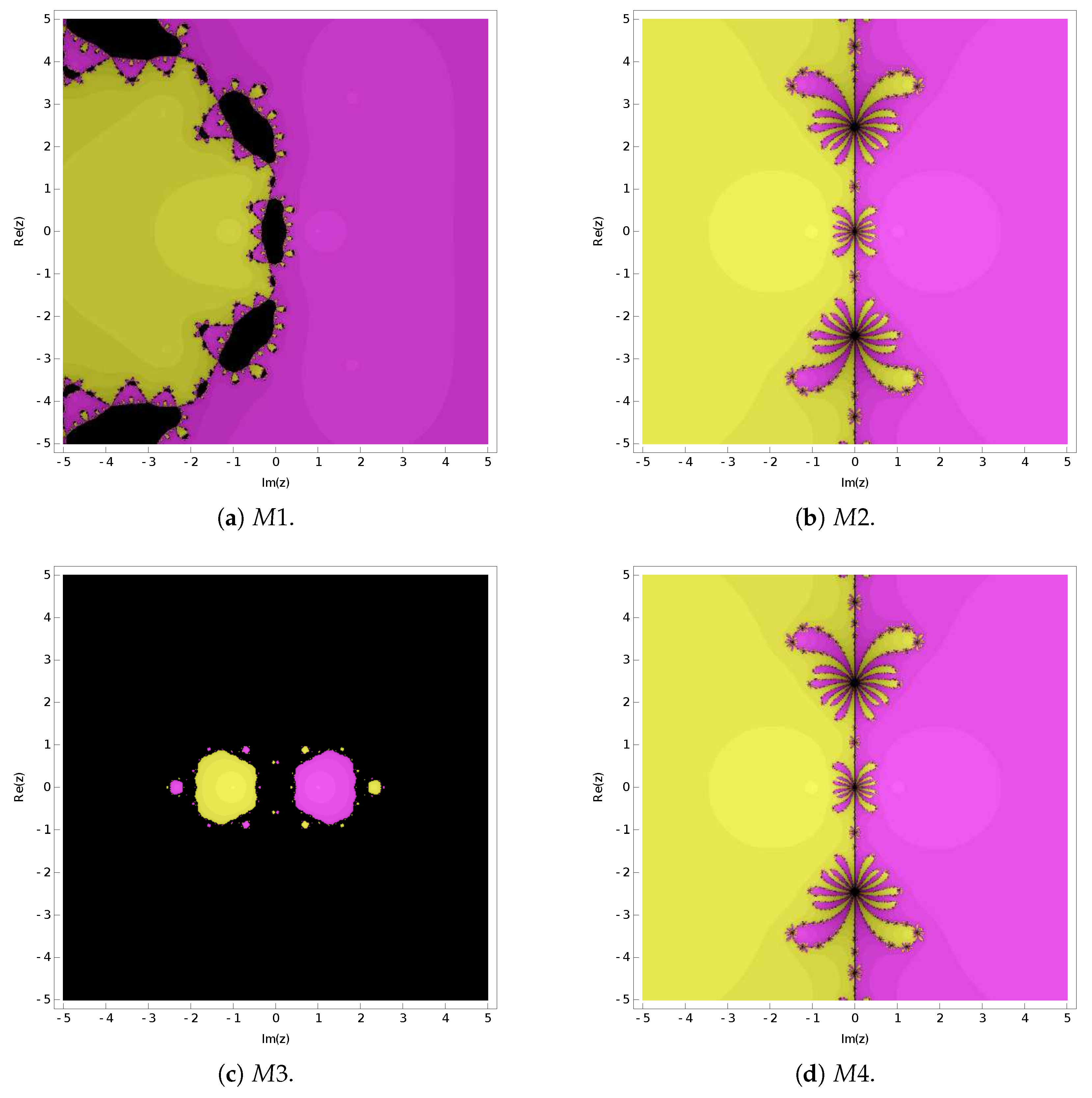
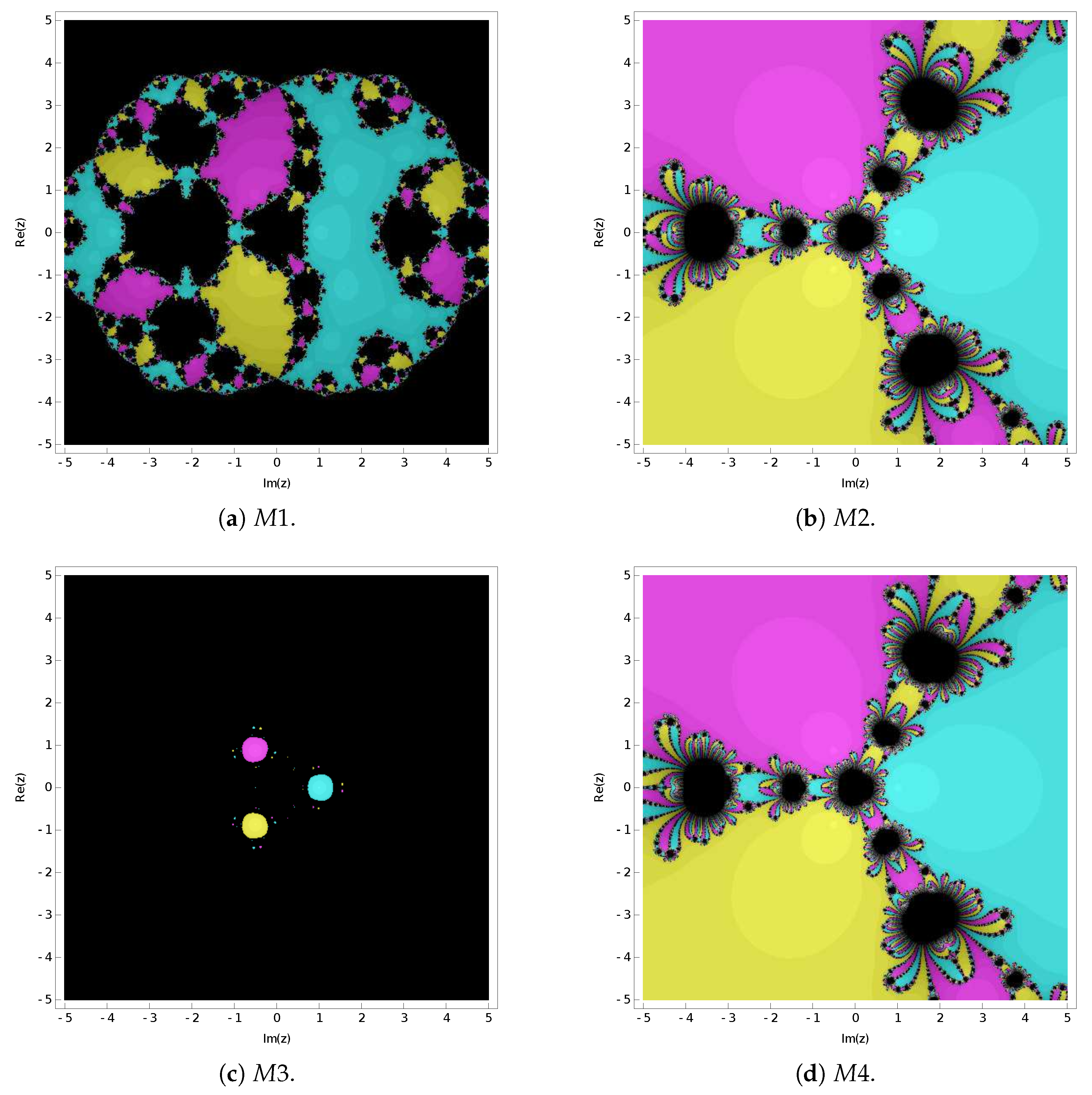
4. Fractals of Attractive Basins

In this section, we will generate fractal plots for Iterative Method (30) under various nonlinear functions to visually illustrate its convergence. Additionally, we will depict the fractal graphs of three sixth-order iterative methods for solving nonlinear equations. The average number of iterations after five iterations were calculated and are, respectively, presented in Figure 1 and Figure 2, as well as

Table 1. Comparison of the average number of iterations after five iterations of Iterative Methods $M1$–$M4$.

	$\mathit{M}1$	$\mathit{M}2$	$\mathit{M}3$	$\mathit{M}4$
$f(x)=x^2-1$	$5.4303$	$3.9349$	$13.243$	$3.9349$
$f(x)=x^3-1$	$11.827$	$7.3072$	$10.359$	$7.2266$

. The different colors in Figure 1 and Figure 2 denote the attractive basins of the different roots. The maximum number of iterations per iteration was set to 25. If the number of iterations exceeded 25 or the iteration sequence failed to converge, it is represented in black.

Let us consider the following sixth-order iterative methods: Iterative Method $M2$, which was proposed by Wang [16]; and $M3$, which was proposed by Behl et al. [17]. As for Iterative Method (30), we will label it as $M4$. Specifically, $M2$ and $M3$ take the following forms, respectively:

$M2$ [16]:

$$\left\{\begin{array}{c}{y}^{(k)}=x^{(k)}-{\mathcal{F}}^{\prime }{(x^{(k)})}^{-1}\mathcal{F}(x^{(k)}),\\ z^{(k)}=y^{(k)}-(2I-{\mathcal{F}}^{\prime }{(x^{(k)})}^{-1}{\mathcal{F}}^{\prime }(y^{(k)})){\mathcal{F}}^{\prime }{(x^{(k)})}^{-1}\mathcal{F}(y^{(k)}),\\ x^{(k+1)}=z^{(k)}-(2I-{\mathcal{F}}^{\prime }{(x^{(k)})}^{-1}{\mathcal{F}}^{\prime }(y^{(k)})){\mathcal{F}}^{\prime }{(x^{(k)})}^{-1}\mathcal{F}(z^{(k)}).\end{array}\right.$$

(52)

$M3$ [17]:

$$\left\{\begin{array}{c}{\displaystyle y^{(k)}=x^{(k)}-\frac{2}{3}{\mathcal{F}}^{\prime }{(x^{(k)})}^{-1}\mathcal{F}(x^{(k)}),}\\ {\displaystyle z^{(k)}{x}^{(k)}-\frac{1}{2}[I+2{\mathcal{F}}^{\prime }(x^{(k)}){(3{\mathcal{F}}^{\prime }(y^{(k)})-{\mathcal{F}}^{\prime }(x^{(k)}))}^{-1}]{\mathcal{F}}^{\prime }{(x^{(k)})}^{-1}\mathcal{F}(x^{(k)}),}\\ x^{(k+1)}=z^{(k)}-2(3{\mathcal{F}}^{\prime }(y^{(k)})-{\mathcal{F}}^{\prime }{(x^{(k)})}^{-1})\mathcal{F}(z^{(k)}).\end{array}\right.$$

(53)

Upon examining Figure 1 and Figure 2, it is evident that the convergence of Iterative Methods $M2$ and $M4$ surpasses that of Iterative Methods $M1$ and $M3$. The data presented in Table 1 further support this observation, with Iterative Method $M4$ demonstrating the lowest average number of iterations over the five iterations.

Building on this conclusion, the subsequent section will involve numerical experiments to compare the performance of Iterative Method $M2$ (52) and Iterative Method $M4$ (30).

5. Numerical Experiments and Practical Applications

In this section, we will utilize Iterative Method (30) to solve nonlinear systems and matrix symbolic functions. We will then compare its performance with that of Iterative Method $M2$ (52), where the advantages of Iterative Method (30) is emphasized. In order to demonstrate the advantages of Iterative Method (30) in terms of computational accuracy, we will also compare the following three other sixth-order iterative methods: $M5$ (54) [18], $M6$ (55) [19], and $M7$ (56) [20]. Method $M5$ is as follows:

$$\left\{\begin{array}{c}{\displaystyle y^{(k)}=x^{(k)}-\frac{1}{2}{\mathcal{F}}^{\prime }{(x^{(k)})}^{-1}\mathcal{F}(x^{(k)}),}\\ z^{(k)}=x^{(k)}+{[{\mathcal{F}}^{\prime }(x^{(k)})-2{\mathcal{F}}^{\prime }(y^{(k)})]}^{-1}[3\mathcal{F}(x^{(k)})-4\mathcal{F}(y^{(k)})],\\ x^{(k+1)}=z^{(k)}+{[{\mathcal{F}}^{\prime }(x^{(k)})-2{\mathcal{F}}^{\prime }(y^{(k)})]}^{-1}\mathcal{F}(z^{(k)}).\end{array}\right.$$

(54)

Method $M6$ is as follows:

$$\left\{\begin{array}{c}{\displaystyle y^{(k)}=x^{(k)}-\frac{2}{3}{\mathcal{F}}^{\prime }{(x^{(k)})}^{-1}\mathcal{F}(x^{(k)}),}\\ {\displaystyle z^{(k)}=x^{(k)}-[\frac{23}{8}-(3+\frac{9}{8}{\mathcal{F}}^{\prime }(y^{(k)})){\mathcal{F}}^{\prime }(y^{(k)})]{\mathcal{F}}^{\prime }{(x^{(k)})}^{-1}\mathcal{F}(x^{(k)}),}\\ {\displaystyle x^{(k+1)}=z^{(k)}-\frac{5}{2}\mathcal{F}(z^{(k)})+\frac{3}{2}\mathcal{F}{(y^{(k)})}^{-1}\mathcal{F}(z^{(k)}).}\end{array}\right.$$

(55)

Method $M7$ is as follows:

$$\left\{\begin{array}{c}{y}^{(k)}=x^{(k)}-\mathcal{F}{[x^{(k)}+\mathcal{F}(x^{(k)}),x-\mathcal{F}(x^{(k)})]}^{-1}\mathcal{F}(x^{(k)}),\\ z^{(k)}=y^{(k)}-{\{2\mathcal{F}[x^{(k)},y^{(k)}]-\mathcal{F}[x^{(k)}+\mathcal{F}(x^{(k)}),x-\mathcal{F}(x^{(k)})]\}}^{-1}\mathcal{F}(y^{(k)}),\\ x^{(k+1)}=z^{(k)}-{\{2\mathcal{F}[x^{(k)},y^{(k)}]-\mathcal{F}[x^{(k)}+\mathcal{F}(x^{(k)}),x-\mathcal{F}(x^{(k)})]\}}^{-1}\mathcal{F}(z^{(k)}).\end{array}\right.$$

(56)

Additionally, we will apply Iterative Method (30) to address practical chemistry problems, thus showcasing its applicability.

5.1. Solving Nonlinear Systems

We will address the following three nonlinear systems (where k represents the number of iterations, the experimental accuracy was 2048, and the experimental results are presented in

Table 2. Experimental results of Problem 1.

The Iterative Method	k	$\parallel {\mathit{x}}^{(\mathit{k})}-{\mathit{x}}^{(\mathit{k}-1)}\parallel$	$\parallel \mathcal{F}({\mathit{x}}^{(\mathit{k})})\parallel$
$M2$	4	$9.193\times {10}^{-158}$	$7.704\times {10}^{-946}$
$M4$	4	$8.793\times {10}^{-240}$	$9.423\times {10}^{-1439}$
$M5$	4	$1.350\times {10}^{-260}$	$1.409\times {10}^{-1239}$
$M6$	4	$2.427\times {10}^{-232}$	$6.265\times {10}^{-1394}$
$M7$	5	$7.121\times {10}^{-144}$	$9.423\times {10}^{-575}$

,

Table 3. Experimental results of Problem 2.

The Iterative Method	k	$\parallel {\mathit{x}}^{(\mathit{k})}-{\mathit{x}}^{(\mathit{k}-1)}\parallel$	$\parallel \mathcal{F}({\mathit{x}}^{(\mathit{k})})\parallel$
$M2$	5	$3.985\times {10}^{-562}$	$1.000\times {10}^{-2048}$
$M4$	5	$1.018\times {10}^{-568}$	$1.000\times {10}^{-2048}$
$M5$	4	$5.015\times {10}^{-138}$	$1.409\times {10}^{-823}$
$M6$	5	$9.737\times {10}^{-569}$	$1.000\times {10}^{-2048}$
$M7$	4	$1.483\times {10}^{-107}$	$2.358\times {10}^{-639}$

and

Table 4. Experimental results of Problem 3.

The Iterative Method	k	$\parallel {\mathit{x}}^{(\mathit{k})}-{\mathit{x}}^{(\mathit{k}-1)}\parallel$	$\parallel \mathcal{F}({\mathit{x}}^{(\mathit{k})})\parallel$
$M2$	5	$2.417\times {10}^{-297}$	$1.111\times {10}^{-1779}$
$M4$	5	$6.170\times {10}^{-464}$	$6.000\times {10}^{-2048}$
$M5$	5	$4.248\times {10}^{-465}$	$3.000\times {10}^{-2048}$
$M6$	6	$9.128\times {10}^{-409}$	$3.000\times {10}^{-2048}$
$M7$	5	$8.615\times {10}^{-290}$	$9.599\times {10}^{-1734}$

):

$Problem1$

$$\left\{\begin{array}{c}{x}_2+x_3+x_4-e^{-x_1}=0,\\ x_1+x_3+x_4-e^{-x_2}=0,\\ x_2+x_1+x_4-e^{-x_3}=0,\\ x_1+x_2+x_3-e^{-x_4}=0.\end{array}\right.$$

(57)

During the iteration, we chose the initial value to be $x^{(0)}={(1.5,1.5,1.5,1.5)}^T$. The solution to the system is ${(2.576\times {10}^{-1},2.576\times {10}^{-1},2.576\times {10}^{-1},2.576\times {10}^{-1})}^T$. The stop criterion is $\parallel x^{(k)}-x^{(k-1)}\parallel <{10}^{-100}$.

$Problem2$

$$\left\{\begin{array}{c}{x}_1^3-sin(x_2)=0,\\ x_2^3-sin(x_1)=0.\end{array}\right.$$

(58)

During the iteration, we chose the initial value to be $x^{(0)}={(1.1,1.1)}^T$. The solution to the system is ${(9.286\times {10}^{-1},9.286\times {10}^{-1})}^T$. The stop criterion is $\parallel x^{(k)}-x^{(k-1)}\parallel <{10}^{-100}$.

$Problem3$

$$\left\{\begin{array}{c}{x}_1-cos(2x_1-{\displaystyle {\sum }_{j=1}^m}{x}_j)=0,\\ x_i-cos(2x_i-{\displaystyle {\sum }_{j=1}^m}{x}_j)=0,1⩽i⩽m.\end{array}\right.$$

(59)

Here, m is the number of equations. During the iteration, we chose the initial value to be $x^{(0)}={(0.1,\cdots ,0.1)}^T$. When $m=6$, the solution to the system is ${(3.131\times {10}^{-1},\cdots ,3.131\times {10}^{-1})}^T$. The stop criterion is $\parallel x^{(k)}-x^{(k-1)}\parallel <{10}^{-100}$.

The experimental results from Table 2, Table 3 and Table 4 show that the convergence accuracy of Iterative Method $M7$ is inferior to the other four iterative methods. Therefore, we will contrast Iterative Methods $M2,M4,M5,$ and $M6$ in the next section by solving a nonlinear matrix sign function.

5.2. Solving the Matrix Sign Function

In this section, we will, respectively, apply Iterative Methods $M2,M4,M5,$ and $M6$ to solve the nonlinear matrix symbolic function $X^2-I=0$, where I represents the identity matrix. Therefore, when solving this function, the corresponding iterative formats for $M2, M4, M5,$ and $M6$ are

•

$$\begin{gathered} X_{n+1}=8192X_n^{19}{[-I+4X_n^2-27X_n^4+120X_n^6-306X_n^8-2174X_n^{12}+4104X_n^{14}-7421X_n^{16} \\ +\mathrm{11,068}{X}_n^{18}+1737X_n^{20}]}^{-1} \end{gathered}$$,

•

$X_{n+1}=1024X_n^{13}{[I-13X_n^2+85X_n^4-305X_n^6+659X_n^8-951X_n^{10}+1303X_n^{12}+245X_n^{14}]}^{-1}$,

•

$X_{n+1}=-{(I+X_n^2)}^3{\left[2X_n^3(3+8X{n}^2+9X_n^4)\right]}^{-1}$,

•

$$\begin{gathered} X_{n+1}=-\mathrm{82,944}{X}_n^{14}(-I+4X_n^4)[-160I+320X_n^2+3408X_n^3+3040X_n^4-6816X_n^5 \\ -2512X_n^6-\mathrm{53,424}{X}_n^7-\mathrm{18,656}{X}_n^8-\mathrm{104,856}{X}_n^9+\mathrm{24,560}{X}_n^{10}+\mathrm{625,584}{X}_n^{11}-\mathrm{960,810}{X}_n^{12} \\ +\mathrm{1,057,896}{X}_n^{13}+\mathrm{1,020,244}{X}_n^{14}-\mathrm{4,451,451}{X}_n^{15}+\mathrm{3,955,646}{X}_n^{16}+\mathrm{55,830}{X}_n^{17} \\ -\mathrm{4,435,280}{X}_n^{18}+\mathrm{5,390,181}{X}_n^{19}+\mathrm{89,000}{X}_n^{20}-\mathrm{3,637,632}{X}_n^{21}+\mathrm{160,768}{X}_n^{22}+\mathrm{872,448}{X}_n^{23} \\ +\mathrm{163,840}{X}_n^{24}]\text{ respectively.} \end{gathered}$$

The experimental results are displayed in

Table 5. Experimental results of the solving matrix sign function.

The Iterative Method	Matrices	n	t
$M2$	1	$nc$	$nc$
	4	$nc$	$nc$
	10	$nc$	$nc$
	15	$nc$	$nc$
$M4$	1	1	$0.008228$
	4	18	$0.040754$
	10	22	$0.051711$
	15	36	$0.089662$
$M5$	1	$nc$	$nc$
	4	$nc$	$nc$
	10	$nc$	$nc$
	15	$nc$	$nc$
$M6$	1	1	$0.035088$
	4	$nc$	$nc$
	10	$nc$	$nc$
	15	$nc$	$nc$

, where n represents the number of iterations, t represents the CPU running time, and $nc$ indicates no convergence. The termination criterion was set to $\parallel X_n^2{-I\parallel }_2⩽{10}^{-100}$.

According to the experimental results in Table 5, it can be seen that Iterative Method $M4$ is superior to $M2,M5,$ and $M6$ in solving the nonlinear matrix symbolic function.

5.3. Practical Applications

The gas equation of the state problem stands out as one of the most crucial challenges in addressing practical chemical problems. In this context, we will apply Theorem 2 from Section 3 to this problem. To begin with, let us consider the following van der Waals equation:

$${\displaystyle \mathcal{F}(V)=(p+\frac{a{n}^2}{V^2})(V-nb)-nRT=0,}$$

(60)

where a = 4.17 atm·L/mol² and b = 0.0371 L/mol. Then, the volume of the container is found by considering the pressure of 945.36 kPa (9.33 atm) and the temperature of 300.2 K with 2 mol nitrogen. Finally, by substituting the data into (60), we obtain

$$\mathcal{F}(V)=9.33V^3-96.9611V^2+16.68V-1.23766=0.$$

In the context of a practical problem, the solution to this nonlinear equation can only be found on $\mathbb{R}$. If we further qualify $\mathcal{U}=[0,0.2]$, then ${\alpha }^{\ast }=0.109171$, where ${\alpha }^{\ast }$ is the result of preserving 6 significant digits for the exact solution. As such, by using Theorem 2, we find

$${\mathcal{D}}_1=15.8667s,{\mathcal{D}}_2=16.3673s,{\mathcal{D}}_3=2.$$

According to Theorem 2, we can finally obtain

$$s_{min}=0.0630251,s_1=0.0415794,s_2=0.0138653,s_3=0.00391481.$$

As such, $r=min\{s_1,s_2,s_3\}=0.0391481$.

In the chemical production process of converting nitrogen–hydrogen feed into ammonia, if the air pressure is 250 atm and the temperature is 500 degrees Celsius, then the following equation can be derived:

$$\mathcal{F}(s)=s^4-7.79075s^3+14.7445s^2+2.511s-1.674.$$

(61)

In a practical context, by limiting the range of solutions to $[0,1]$, we know that the root of Equation (61) is ${\alpha }^{\ast }=0$. Then, we have

$${\mathcal{D}}_1=2.59403s,{\mathcal{D}}_2=3.28225s,{\mathcal{D}}_3=2.$$

According to Theorem 2, we can finally obtain

$$s_{min}=0.385501,s_1=0.236119,s_2=0.0737151,s_3=0.02006.$$

As such, $r=min\{s_1,s_2,s_3\}=0.02006$.

6. Conclusions and Discussion

In this paper, a class of iterative methods for solving nonlinear systems (1) was presented. Through the proof results in Theorem 1, we established that, when $\mathcal{P}=2$ and $\mathcal{Q}=1$, Iterative Method (1) can reach a sixth-order convergence, which is Iterative Method (30).

During the proof of Theorem 1, we noticed that this convergence process has a high limitation on the existence of the higher derivatives of functions. But not all functions have higher derivatives. Therefore, we discussed the local convergence of Iterative Method (30) in Section 3. By using the $\omega$-continuity condition on the first-order Fréchet derivative in Banach space, we established the conditions for a local convergence of Iterative Method (30), thus avoiding the discussion of the higher-order derivative of the function.

Finally, by drawing the attractive basin of Iterative Method (30)—as well as by comparing it with the average number of iterations of five cycles for the known sixth-order iterative methods $M1$, $M2$, and $M3$ for solving nonlinear systems—it was shown that the new Iterative Method $M4$ (30) is superior to the other three iterative methods in terms of convergence and average number of iterations. In the experiment where nonlinear systems were solved, it was also shown that the convergence accuracy of Iterative Method (30) is better than that of Iterative Method $M7$. Furthermore, when employing Iterative Methods $M2,M4,M5,$ and $M6$ to simultaneously solve the nonlinear matrix symbolic function, it is evident that $M4$ exhibits broader applicability. Through leveraging the local convergence established in Theorem 2 for Iterative Method $M4$, we proceeded to address the practical chemical problems. Through these experiments, we have objectively demonstrated the plausibility of our proposal iterative method.

Building upon the foundation laid in this paper, our future focus will be on proposing diverse forms of iterative methods with higher convergence orders. This will involve analyzing their local convergence, semi-local convergence, and employing fractal theory to study their stability.

References

1. Roman, J.G.; Adam, W.; Karol, M. An adaptive Dynamic Relaxation method for solving nonlinear finite element problems. Application to brain shift estimation. Int. J. Numer. Methods Biomed. 2011, 27, 173–185. [Google Scholar]
2. Zhang, Y.; Kou, X.; Song, Z.; Fan, Y.; Mohammed, U.; Vishal, J. Research on logistics management layout optimization and real-time application based on nonlinear programming. Nonlinear Dyn. 2021, 10, 526–534. [Google Scholar] [CrossRef]
3. Hajime, K.; Hajime, K. Estimation method for inverse problems with linear forward operator and its application to magnetization estimation from magnetic force microscopy images using deep learning. Inverse Probl. Sci. Eng. 2021, 29, 2131–2164. [Google Scholar]
4. Muhammad, A.; Iitaf, H.; Masood, A. A finite-difference and Haar wavelets hybrid collocation technique for non-linear inverse Cauchy problems. Inverse Probl. Sci. Eng. 2022, 30, 121–140. [Google Scholar]
5. Anakhaev, K.N. The Problem of Nonlinear Cantilever Bending in Elementary Functions. Mech. Solids 2022, 57, 997–1005. [Google Scholar] [CrossRef]
6. Ortega, J.M.; Rheinboldt, W.C. Iterative Solution of Nonlinear Equations in Several Variables; Academic Press: New York, NY, USA, 1970. [Google Scholar]
7. Traub, J.F. Iterative Methods for the Solution of Equations; Prentice-Hall: Englewood Cliffs, NJ, USA, 1964. [Google Scholar]
8. Cordero, A.; Miguel, A.L.S.; Torregrosa, J.R. Dynamics and stability on a family of fourth-order optimal iterative methods. Algorithms 2022, 15, 387. [Google Scholar] [CrossRef]
9. Argyros, I.K.; Regmi, S.; John, J.A.; Jayaraman, J. Extended Convergence for Two Sixth Order Methods under the Same Weak Conditions. Foundations 2023, 3, 127–139. [Google Scholar] [CrossRef]
10. Sabban, A. Novel Meta-Fractal Wearable Sensors and Antennas for Medical, Communication, 5G, and IoT Applications. Fractal Fract. 2024, 8, 100. [Google Scholar] [CrossRef]
11. Wang, X.; Chen, X.; Li, W. Dynamical Behavior Analysis of an Eighth-Order Sharma’s Method. Int. J. Biomath. 2023, 2350068. [Google Scholar] [CrossRef]
12. Wang, X.; Xu, J. Conformable vector Traub’s method for solving nonlinear systems. Numer. Algorithms 2024. [Google Scholar] [CrossRef]
13. Argyros, I.K.; Magreñán, Á.A. A study on the local convergence and the dynamics of Chebyshev-Halley-type methods free from second derivative. Numer. Algorithms 2016, 71, 1–23. [Google Scholar] [CrossRef]
14. Saeed, K.M.; Remesh, K.; George, S.; Padikkal, J.; Argyros, I.K. Local Convergence of Traub’s Method and Its Extensions. Fractal Fract. 2023, 7, 98. [Google Scholar] [CrossRef]
15. Amat, S.; Argyros, I.K.; Busquier, S.; Magreñán, Á.A. Local convergence and the dynamics of a two-point four parameter Jarratt-like method under weak conditions. Numer. Algorithms 2017, 74, 371–391. [Google Scholar] [CrossRef]
16. Wang, X.; Li, Y. An Efficient Sixth-Order Newton-Type Method for Solving Nonlinear Systems. Algorithms 2017, 10, 45. [Google Scholar] [CrossRef]
17. Behl, R.; Argyros, I.K.; Machado, J.A.T. Ball Comparison between Three Sixth Order Methods for Banach Space Valued Operators. Mathematics 2020, 8, 667. [Google Scholar] [CrossRef]
18. Cordero, A.; Torregrosa, J.R.; Vassileva, M.P. Pseudocomposition: A technique to design predictor-corrector methods for systems of nonlinear equations. Appl. Math. Comput. 2012, 218, 11496–11504. [Google Scholar] [CrossRef]
19. Petković, M.S.; Neta, B.; Petković, L.D.; Džunić, J. Multipoint Methods for Solving Nonlinear Equations; Elsevier: New York, NY, USA, 2013. [Google Scholar]
20. Grau-Sánchez, M.; Noguera, M.; Amat, S. On the approximation of derivatives using divided difference operators preserving the local convergence order of iterative methods. J. Comput. Appl. Math. 2013, 237, 263–272. [Google Scholar] [CrossRef]
Figure 1. The attractive basins of Iterative Methods M 1 M 4 under the nonlinear function f ( x ) = x 2 1 .
Fractalfract 08 00133 g001
Figure 2. The attractive basins of Iterative Methods M 1 M 4 under the nonlinear function f ( x ) = x 3 1 .
Fractalfract 08 00133 g002