Article

Solutions to Fractional q-Kinetic Equations Involving Quantum Extensions of Generalized Hyper Mittag-Leffler Functions

1
Department of Mathematics, College of Science, King Khalid University, Abha 61413, Saudi Arabia
2
Department of Mathematics, Faculty of Science, South Valley University, Qena 83523, Egypt
*
Author to whom correspondence should be addressed.
Fractal Fract. 2024, 8(1), 58; https://doi.org/10.3390/fractalfract8010058
Submission received: 13 December 2023 / Revised: 4 January 2024 / Accepted: 9 January 2024 / Published: 16 January 2024

Abstract

:
This manuscript focuses on new generalizations of q-Mittag-Leffler functions, called generalized hyper q-Mittag-Leffler functions, and discusses their regions of convergence and various fractional q operators. Moreover, the solutions to the q-fractional kinetic equations in terms of the investigated generalized hyper q-Mittag-Leffler functions are obtained by applying the q-Sumudu integral transform. Furthermore, we present solutions obtained as numerical graphs using the MATLAB 2018 program.

1. Introduction

Fractional differential equations (FDEs) have received tremendous interest in recent decades. They play a significant role in describing real-world phenomena such as energy [1], financial systems [2], hydrologic modeling [3], electrochemistry [4], mathematical biology [5], and signal processing [6], amongst others [7,8]. Later on, fractional kinetic equations can be seen as an essential part of fractional differential equations, where a wide range of analytical and numerical methods can be used to obtain their solutions. Also, several ways to study the extension and development of fractional kinetic equations involving various special functions have been presented. For example, we refer to contemporary works by Agarwal et al. [9], Saxena et al. [10], Akel et al. [11], Hidan et al. [12], Almalkia and Abdalla [13], Kolokoltsov and Troeva [14], Habenom et al. [15] and Abdalla and Akel [16].
On the other hand, fractional q-differential equations are an extension of the fractional differential equations in quantum calculus (or q-calculus) frameworks. Nowadays, the solution to the quantum analogue (or q-analogue) of the fractional kinetic equation with the Riemann–Liouville fractional q-integral operator is acquired using the technique of a q-analogue of the Laplace transform, which has been discussed by Garg and Chanchlani [17]. Meanwhile, Purohit and Faruk Uçar investigated an application of the q-Sumudu transform for fractional q-kinetic equations in [18]. Recently, Bairwa et al. [19] obtained the solution to the fractional q-kinetic equation pertaining to the generalized q-Mittag-Leffler function via the q-Sumudu transform. In a similar vein, Abujarad al. [20] introduced and investigated the solutions to q-fractional kinetic equations, including the generalized hyper Bessel function, using the q-Shehu transform.
Motivated by the previous works, we define new quantum extensions of the generalized hyper Mittag-Leffler functions in this article and establish their properties and applications in generalized fractional q-kinetic equations. This work’s organization is as follows. Section 2 presents the basic concepts of q-calculus and reviews the versions of Mittag-Leffler functions that are required in the following sections. In Section 3, we introduce the two q-analogues of the generalized hyper Mittag-Leffler functions and study the convergence properties of these functions for  | q | < 1 . Some of the fractional q-operators of the generalized hyper q-Mittag-Leffler functions using the Caputo fractional q-derivatives, the Hilfer fractional q-derivatives, the Kober q-integrals, and the Riemann-Liouville q-integrals are proposed in Section 4. In Section 5, we find the solutions to the q-fractional kinetic equations involving the generalized hyper q-Mittag-Leffler functions by using the q-Sumudu transform. In Section 6, we point out the graphical representations of the primary obtained solutions in Section 4 using the MATLAB program. Eventually, we exhibit some concluding remarks in Section 7.

2. Mathematical Preliminaries

2.1. Some Basic Concepts of q-Calculus

The quantum calculus (q-calculus) is the q extension of ordinary calculus. The theory of q-calculus operators has recently been applied in modern sciences (e.g., see [21,22,23]).
Now, we recall some of the basic concepts and related details of q-calculus which will be used in the current study.
Definition 1
(See [24]). Given a value of  0 < | q | < 1 , the q-number  [ κ ] q is defined as
[ κ ] q : = q κ 1 q 1 , q 1 , κ , q = 1 , κ R .
For  κ N , the q-factorial  [ κ ] q ! is given by
[ κ ] q ! = [ κ ] q [ κ 1 ] q [ 1 ] q , κ N , 1 , κ = 0 .
Definition 2
(See [24]). For  0 < | q | < 1 , the q-analogue of the common Pochhammer symbols (q-shifted factorials) are given as follows:
θ ; q κ = ı = 0 κ 1 1 θ q ı , κ N , 1 , κ = 0 ,
θ ; q = ı = 0 1 θ q ı , θ C
and
θ ; q η = θ ; q θ q η ; q , θ , η C .
Definition 3
(See [24]). For  0 < | q | < 1 , the q-analogue of  ( u v ) q κ is given as follows:
u v q κ = u κ v / u ; q κ = u κ v / u ; q v q κ / u ; q , u 0 .
Definition 4
(See [24,25]). For  0 < | q | < 1 , the q-gamma function is defined by
Γ q ( θ ) = ( q ; q ) q θ ; q ( 1 q ) 1 θ = ( q ; q ) θ 1 ( 1 q ) θ 1 Re ( θ ) > 0 ,
where  lim q 1 Γ q ( θ ) = Γ ( θ ) and  Γ ( θ ) is the classical gamma function
Γ ( θ ) = 0 τ θ 1 e τ d τ , θ C Z .
Note that
Γ q ( θ + 1 ) = [ θ ] q Γ q ( θ ) = [ θ ] q ! Re ( θ ) > 0 .
Moreover, the q-analogue of Stirling’s asymptotic formula for the q-gamma function (Equation (7)) is defined in [25] by
Γ q ( θ ) ( 1 + q ) 1 2 Γ q 2 ( 1 2 ) ( 1 q ) 1 2 θ e Υ q ( θ ) ,
where  Υ q ( θ ) = φ q θ 1 q q θ , 0 < φ < 1 .
Definition 5
(See [24,25]). For  0 < q < 1 , the q-beta function is defined by
B q ( θ , φ ) = Γ q ( θ ) Γ q ( φ ) Γ q ( θ + φ ) , Re ( θ ) > 0 , Re ( φ ) > 0 .
Definition 6
(See [24]). The q-derivative  D q Ψ of a function  Ψ ( η ) is defined as
D q Ψ ( η ) = Ψ ( η ) Ψ ( q η ) η ( 1 q ) , η 0 , q 1 ,
and  D q Ψ ( 0 ) = Ψ ( 0 ) , provided  Ψ ( 0 ) exists.
We observe that
D q s ( η r ) = Γ q ( r + 1 ) Γ q ( r s + 1 ) η r s , r , s N ,
And if  Ψ ( η ) is differentiable, then one has
lim q 1 D q Ψ ( η ) = lim q 1 Ψ ( q η ) Ψ ( η ) η ( q 1 ) = d Ψ ( η ) d η .
Definition 7
(See [24]). For  0 < | q | < 1 , the q-Jackson integral is defined as
0 η f ( τ ) d q τ = ( 1 q ) η ι = 0 q ι f ( q ι η ) ,
provided the sum converges absolutely.
Definition 8
(See [21,22]). The Riemann–Liouville fractional q-integral operator is defined by
I q ν f ( η ) : = 1 Γ q ( ν ) 0 η η q u q ν 1 f ( u ) d q u , Re ( ν ) > 0 .
It is clear that
I q ν [ η μ ] = Γ q ( 1 + μ ) Γ q ( 1 + μ + ν ) η μ + ν , μ ( 1 , ) .
Definition 9
(See [21,22]). The Kober fractional q-integral operator is defined by
I q μ , ν f ( η ) : = η μ ν Γ q ( ν ) 0 η η q u q ν 1 u μ f ( u ) d q u , Re ( μ ) > 0 .
Definition 10
(See [21,22]). The Caputo fractional q-derivative is defined by
c D q ν [ f ] ( η ) = I q 1 ν D q [ f ] ( η ) = 1 Γ q ( 1 ν ) 0 η ( η q τ ) q ν D q f ( τ ) d q τ , Re ( ν ) > 0 .
Definition 11
(See [21,22]). The Hilfer fractional q-derivative of an order ν and of type μ is defined by
D q μ , ν [ f ] ( η ) = I q μ ( 1 ν ) D q I q ( 1 m u ) ( 1 ν ) [ f ] ( η ) , 0 < ν < 1 , 0 μ 1 .
Definition 12.
For  0 < | q | < 1 , the two q-analogues of the exponential function are given in [22,24] as follows:
E q ( η ) = ι = 0 η ι ( q ; q ) ι = 1 ( η ; q ) , | η | < 1 ,
and
E q ( η ) = ι = 0 ( 1 ) ι q ι ( ι 1 ) / 2 η ι ( q ; q ) ι = ( η ; q ) , | η | < .

2.2. Some Versions of the Mittag-Leffler Function

Following Swedish mathematician Gosta Mittag-Leffler [26], the Mittag-Leffler (M-L) function is defined by
E α ( ξ ) = k = 0 ξ k Γ ( k α + 1 ) , ξ , α C , Re ( α ) > 0 ,
where  Γ ( . ) is the gamma function (Equation (8)).
This function is the direct generalization of the exponential function
E 1 ( ξ ) = e ξ = k = 0 ξ k k ! ξ C .
Various generalizations of the M-L function are provided below.
Generalizations of  E α ( ξ ) first appeared in a 1905 work by Wiman [27] as
E α , β ( ξ ) = k = 0 ξ k Γ ( k α + β ) ξ , α , β C , Re ( α ) > 0 , Re ( β ) > 0 .
The function  E α , β ( ξ ) is the natural extension of certain functions like hyperbolic trigonometric functions, among others (refer to [26,27]).
Prabhakar [28] introduced the following extension of Equation (23):
E α , β δ ( ξ ) = k = 0 ( δ ) k Γ ( k α + β ) ξ k k ! , ( ξ , α , β , δ C , Re ( α ) > 0 , Re ( β ) > 0 ) ,
where  ( δ ) m denotes the usual Pochhammer symbol defined by
( δ ) k = Γ ( δ + m ) Γ ( δ ) = δ ( δ + 1 ) . . . ( δ + m 1 ) , m N , δ C 1 , m = 0 ; δ C { 0 } ,
and  Γ ( . ) is the gamma function defined by Equation (8).
In [29], Shukla and Prajapati presented the following function:
E α , β δ , ν ( ξ ) = k = 0 ( δ ) ν k Γ ( k α + β ) ξ k k ! , ( ξ , α , β , δ C , Re ( α ) > 0 , Re ( β ) > 0 , ν ( 0 , 1 ) N ) ,
where  ( δ ) ν k is the generalized Pochhammer symbol given as follows:
( δ ) ν k = Γ ( δ + k ν ) Γ ( δ ) = k ν k j = 1 k δ + j 1 k , k N .
Another generalization of Equation (23) according to Salim [30,31] is given by
E α , β δ , ν ( ξ ) = k = 0 ( δ ) k Γ ( k α + β ) ( ν ) k ξ k k ! , ( ξ , α , β , δ , ν C , Re ( α ) > 0 , Re ( β ) > 0 , Re ( δ ) > 0 , Re ( ν ) > 0 ) .
On the other hand, we will mention some q-analogues of the Mittag-Leffler-type functions functions.
Jain [32] introduced a q-analogue of the generalized Mittag-Leffler function:
E α ( w ; q ) = h = 0 w h Γ q ( α h + 1 ) , ( Re ( α ) > 0 ) .
Mansour [33] introduced a new form of a q-analogue of the Mittag-Leffler function, given by
E α , δ ( w ; q ) = h = 0 w h Γ q ( h α + δ ) , α > 0 , δ C , ( | w | < ( 1 q ) α ) .
Meanwhile, Sharma and Jain [34] presented and established the q-analogue of the Mittag-Leffler function below:
E α , δ γ ( w ; q ) = h = 0 ( q γ ; q ) h Γ q ( h α + δ ) · w h ( q ; q ) h , | w | < ( 1 q ) α ,
where  α > 0 , γ > 0 , δ , w C , and  | q | < 1 .
Furthermore, Purohit and Kalla [35] defined and investigated another generalization of Equation (30) in the form
E α , δ γ ( w ; q ) = h = 0 q h ( h 1 ) / 2 ( q γ ; q ) h Γ q ( h α + δ ) · w h ( q ; q ) h , | w | < ( 1 q ) α ,
where  α > 0 , γ > 0 , δ , w C , and  | q | < 1 .
Further recent generalizations and applications of the q-Mittag-Leffler function can be found in [36,37,38,39].

3. The Generalized Hyper  q -Mittag-Leffler Functions

Motivated by the studies quoted in Section 2.2, we introduce here the two q-analogues of the generalized hyper Mittag-Leffler function in the following definition:
Definition 13.
Let  α ,   β ,   λ s ,   δ r C such that  Re ( α ) > 0 ,   Re ( λ s ) > 0 , and  Re ( δ r ) > 0 for the finite sets  s 1 , 2 , , d and  r 1 , 2 , , h . Let  λ = ( λ 1 , λ 2 , , λ d ) δ = ( δ 1 , δ 2 , , δ h ) , and  0 < | q | < 1 . Then, the function
E α , β , δ λ ( w ; q ) = = 0 Π s = 1 d Γ q ( λ s + ) Γ q ( α + β ) Π r = 1 h Γ q ( δ r + ) · w ( q ; q ) ,
is called the small generalized hyper q-Mittag-Leffler function. Similarly, the large generalized hyper q-Mittag-Leffler function is defined as follows:
E α , β , δ λ ( w ; q ) = = 0 ( 1 ) q ( 1 ) / 2 Π s = 1 d Γ q ( λ s + ) Γ q ( α + β ) Π r = 1 h Γ q ( δ r + ) · w ( q ; q ) .
Alternatively, in light of the definition of the q-gamma function in Equation (7), we can rewrite Equations (33) and (34) in the respective forms
E α , β , δ λ ( w ; q ) = = 0 q α + β ; q Π r = 1 h q δ r + ; q Π s = 1 k q λ s + ; q Π s = 1 k Π r = 1 h q δ r λ s + α + β ; q · w ( q ; q )
and
E α , β , δ λ ( w ; q ) = = 0 ( 1 ) q ( 1 ) / 2 q α + β ; q Π r = 1 h q δ r + ; q Π s = 1 k q λ s + ; q Π s = 1 k Π r = 1 h q δ r λ s + α + β ; q · w ( q ; q ) .
Remark 1.
We note the following special cases for Equations (33) and (34):
  • By putting  λ = λ 1 and  δ = δ 1 in Equations (33) and (34), we obtain the following generalized q-Mittag-Leffler functions:
    e α , β , δ 1 λ 1 ( w ; q ) = = 0 Γ q ( λ 1 + ) d Γ q ( α + β ) Γ q ( δ 1 + ) h · w ( q ; q ) ,
    and
    E α , β , δ 1 λ 1 ( w ; q ) = = 0 ( 1 ) q ( 1 ) / 2 Γ q ( λ 1 + ) d Γ q ( α + β ) Γ q ( δ 1 + ) h · w ( q ; q ) .
  • By setting  q 1 in Equations (33) and (34), we reduce them to the following generalized hyper Mittag-Leffler function:
    E α , β , δ λ ( w ) = = 0 Π s = 1 d Γ ( λ s + ) Γ ( α + β ) Π r = 1 h Γ ( δ r + ) · w ! ,
    which is a generalization of the Mittag-Leffler functions defined by Equations (21)–(24) and (26).
  • By taking  d = h = 1 in Equations (37) and (38), we give the following generalized q-Mittag-Leffler functions with four parameters:
    e α , β , δ 1 λ 1 ( w ; q ) = = 0 Γ q ( λ 1 + ) Γ q ( α + β ) Γ q ( δ 1 + ) · w ( q ; q )
    and
    E α , β , δ 1 λ 1 ( w ; q ) = = 0 ( 1 ) q ( 1 ) / 2 Γ q ( λ 1 + ) Γ q ( α + β ) Γ q ( δ 1 + ) · w ( q ; q ) .
    which generalize the Mittag-Leffler functions defined by Equations (20), (29), and (32).
  • When  d = h = 1 and  δ 1 = λ 1 in Equations (40) and (41), we obtain the following generalized q-Mittag-Leffler functions:
    E α , β ( w ; q ) = = 0 1 Γ q ( α + β ) · w ( q ; q )
    and
    E α , β ( w ; q ) = = 0 ( 1 ) q ( 1 ) / 2 Γ q ( α + β ) · w ( q ; q ) .
We now discuss the convergence properties of the generalized hyper q-Mittag-Leffler functions defined in Equations (33) and (34). First, the following theorem ensures the convergence and order of Equation (34):
Theorem 1.
Under the conditions and hypothesis in Definition 13,  E α , β , δ λ ( w ; q ) is an entire function for  0 < | q | < 1 , and its order is equal to zero.
Proof. 
For this proof, we can rewrite Equation (34) in the form
E α , β , δ λ ( w ; q ) = = 0 ( 1 ) q ( 1 ) / 2 Π s = 1 d Γ q ( λ s + ) Γ q ( α + β ) Π r = 1 h Γ q ( δ r + ) · w ( q ; q ) = = 0 U q w ,
where
U q = ( 1 ) q ( 1 ) / 2 Π s = 1 d Γ q ( λ s + ) Γ q ( α + β ) Π r = 1 h Γ q ( δ r + ) · 1 ( q ; q ) .
Using the relation in Equation (9), and after simplifications, we arrive at the radius of regularity R of the above series as follows:
1 R = lim | U q | lim | ( 1 ) q ( 1 ) / 2 ( 1 + q ) 1 2 Γ q 2 ( 1 2 ) ( 1 q ) 1 2 ( α + β ) e Υ q ( α + β ) | 1 × | Π s = 1 d ( 1 + q ) 1 2 Γ q 2 ( 1 2 ) ( 1 q ) 1 2 ( λ s + ) e Υ q ( λ s + ) Π r = 1 h ( 1 + q ) 1 2 Γ q 2 ( 1 2 ) ( 1 q ) 1 2 ( δ r + ) e Υ q ( δ r + ) | 1 × | 1 ( 1 + q ) 1 2 Γ q 2 ( 1 2 ) ( 1 q ) 1 2 e Υ q ( + 1 ) | 1 lim | q ( 1 ) / 2 | = 0 , 0 < | q | < 1 ,
where  Υ q is defined in Equation (9). Therefore, we have  R = , and hence the function  E α , β , δ λ ( w ; q ) is an entire function. Now, we calculate the order of the entire function  E α , β , δ λ ( w ; q ) as follows (see [21,22]):
ρ E α , β , δ λ ( w ; q ) = lim sup ln ln 1 | U q | ,
which given from Equation (45) as
ln 1 | U q | = ln Γ q ( α + β ) Π r = 1 h Γ q ( δ r + ) ( 1 q ) Γ q ( + 1 ) q ( 1 ) / 2 Π s = 1 d Γ q ( λ s + ) = ln | Γ q ( α + β ) | + ln | Π r = 1 h Γ q ( δ r + ) | + ln | Γ q ( + 1 ) | + ln | 1 q | ( 1 ) / 2 ln | q | ln | Π s = 1 d Γ q ( λ s + ) | .
Then, in light of Equation (7), we see that
ln | Γ q ( α + β ) | = ln | ( q ; q ) q ( α + β ) ; q ( 1 q ) 1 ( α + β ) | = ln | ( q ; q ) | ln | q ( α + β ) ; q | + ( 1 ( Re ( α ) + Re ( β ) ) ) ln | ( 1 q ) | .
According to [21], we observe that
ln | q ( α + β ) ; q | = ln m = 0 | 1 q ( α + β + m ) | = ln lim ω m = 0 ω | 1 q ( α + β + m ) | = lim ω m = 0 ω ln | 1 q ( α + β + m ) | = m = 0 ln | 1 q ( α + β + m ) | m = 0 q ( Re ( α + β ) + m ) = q ( Re ( α + β ) ) 1 q .
Consequently, from Equation (47), we have
lim ln | Γ q ( α + β ) | ln = 0 .
Thus, using the above technique in Equation (46), one would obtain
lim ln 1 | U q | ln = .
Hence,  ρ E α , β , δ λ ( w ; q ) = 0 . This completes the proof of Theorem 1. □
Second, the following result includes the absolute convergence of Equation (33):
Theorem 2.
Under the conditions and hypothesis in Definition 13, the function  E α , β , δ λ ( w ; q ) (Equation (33)) converges absolutely for  | w | < ( 1 q ) α with  0 < | q | < 1 .
Proof. 
To prove that we can rewrite Equation (33) as
E α , β , δ λ ( w ; q ) = = 0 Π s = 1 d Γ q ( λ s + ) Γ q ( α + β ) Π r = 1 h Γ q ( δ r + ) · w ( q ; q ) = = 0 U q w ,
where
U q = Π s = 1 d Γ q ( λ s + ) Γ q ( α + β ) Π r = 1 h Γ q ( δ r + ) · 1 ( 1 q ) Γ q ( + 1 ) .
using the relation in Equation (9), and after calculations, it follows that
1 R = lim | U q | lim | 1 ( 1 + q ) 1 2 Γ q 2 ( 1 2 ) ( 1 q ) 1 2 ( α + β ) e Υ q ( α + β ) | 1 × | Π s = 1 d ( 1 + q ) 1 2 Γ q 2 ( 1 2 ) ( 1 q ) 1 2 ( λ s + ) e Υ q ( λ s + ) Π r = 1 h ( 1 + q ) 1 2 Γ q 2 ( 1 2 ) ( 1 q ) 1 2 ( δ r + ) e Υ q ( δ r + ) | 1 × | 1 ( 1 + q ) 1 2 Γ q 2 ( 1 2 ) ( 1 q ) 1 2 e Υ q ( + 1 ) | 1 lim | Π r = 1 h Π s = 1 d ( 1 q ) λ s + δ r + α 1 | 1 lim | ( 1 q ) α | .
Thus, the function  E α , β , δ λ ( w ; q ) is convergent for  | w | < ( 1 q ) α if  0 < | q | < 1 . We thus arrive at the required result. □
Remark 2.
According to Remark 1, many particular cases can be inserted by Theorem 1 and Theorem 2.

4. Fractional  q -Calculus Approach

In this section, we present some of the fractional q-operators of the generalized hyper q-Mittag-Leffler functions in Equations (33) and (34) in the following theorems:
Theorem 3
(Caputo fractional q-derivatives). The Caputo fractional q-derivatives of the generalized hyper q-Mittag-Leffler functions in Equations (33) and (34) are the following respective equations:
c D q ν E α , β , δ λ ( w ν ; q ) = w ν = 0 Γ q ( 1 + ν ) Π s = 1 d Γ q ( λ s + ) Γ q ( α + β ) Γ q ( 1 ν + ν ) Π r = 1 h Γ q ( δ r + ) · w ν ( q ; q ) ,
and
c D q ν E α , β , δ λ ( w ν ; q ) = w ν = 0 ( 1 ) q ( 1 ) / 2 Γ q ( 1 + ν ) Π s = 1 d Γ q ( λ s + ) Γ q ( α + β ) Γ q ( 1 ν + ν ) Π r = 1 h Γ q ( δ r + ) · w ν ( q ; q ) .
Proof. 
By applying Equation (17) to Equation (33), we have
c D q ν E α , β , δ λ ( w ν ; q ) = = 0 Π s = 1 d Γ q ( λ s + ) ( q ; q ) Γ q ( α + β ) Π r = 1 h Γ q ( δ r + ) · c D q ν [ w ν ] = = 0 Π s = 1 d Γ q ( λ s + ) ( q ; q ) Γ q ( α + β ) Π r = 1 h Γ q ( δ r + ) · I q ν 1 D q [ w ν ] .
Using Equations (12) and (15), one finds
c D q ν E α , β , δ λ ( w ν ; q ) = = 0 Π s = 1 d Γ q ( λ s + ) ( q ; q ) Γ q ( α + β ) Π r = 1 h Γ q ( δ r + ) · [ ν ] q I q ν 1 [ w ν 1 ] = = 0 Π s = 1 d Γ q ( λ s + ) ( q ; q ) Γ q ( α + β ) Π r = 1 h Γ q ( δ r + ) · [ ν ] q Γ q ( ν ) Γ q ( 1 ν + ν ) w ν ν = = 0 Π s = 1 d Γ q ( λ s + ) ( q ; q ) Γ q ( α + β ) Π r = 1 h Γ q ( δ r + ) · Γ q ( 1 + ν ) Γ q ( 1 ν + ν ) w ν ν .
This is the required result (Equation (53)). Similarly, Equation (54) can be proven. □
Theorem 4
(Hilfer fractional q-derivatives). The Hilfer fractional q-derivatives of the generalized hyper q-Mittag-Leffler functions in Equations (33) and (34) are the following respective equations:
D q ν , μ E α , β , δ λ ( w ν ; q ) = w ν = 0 Γ q ( 1 + ν ) Π s = 1 d Γ q ( λ s + ) Γ q ( α + β ) Γ q ( 1 ν + ν ) Π r = 1 h Γ q ( δ r + ) · w ν ( q ; q ) ,
and
D q ν , μ E α , β , δ λ ( w ν ; q ) = w ν = 0 ( 1 ) q ( 1 ) / 2 Γ q ( 1 + ν ) Π s = 1 d Γ q ( λ s + ) Γ q ( α + β ) Γ q ( 1 ν + ν ) Π r = 1 h Γ q ( δ r + ) · w ν ( q ; q ) .
where  D q ν , μ is the Hilfer fractional q-differential operator (Equation (18)).
Proof. 
By applying Equation (18) to the function  f ( w ) = w ν , we obtain
D q ν , μ [ w ν ] = I q μ ( 1 ν ) D q I q ( 1 μ ) ( 1 ν ) [ w ] = I q μ ( 1 ν ) D q Γ q ( 1 + ν ) Γ q 1 + ν + ( 1 μ ) ( 1 ν ) w ( 1 μ ) ( 1 ν ) + ν = I q μ ( 1 ν ) Γ q ( 1 + ν ) Γ q 1 + ν + ( 1 μ ) ( 1 ν ) × ( 1 μ ) ( 1 ν ) + ν q w ( 1 μ ) ( 1 ν ) + ν 1 = Γ q ( 1 + ν ) Γ q 1 + ν + ( 1 μ ) ( 1 ν ) ( 1 μ ) ( 1 ν ) + ν q × Γ q ( ( 1 μ ) ( 1 ν ) + ν ) Γ q ( 1 μ ) ( 1 ν ) + ν + μ ( 1 ν ) w ( 1 μ ) ( 1 ν ) + ν + μ ( 1 ν ) 1 = Γ q ( 1 + ν ) Γ q 1 ν + ν w ν ( 1 ) .
This leads directly to Equations (55) and (56). □
Theorem 5
(Kober q-integrals). If  E α , β , δ λ ( w ; q ) and  E α , β , δ λ ( w ; q ) are the generalized hyper q-Mittag-Leffler functions of Equations (33) and (34), respectively, then their Kober fractional q-integrals are
I q ν , μ E α , β , δ λ ( w ; q ) = = 0 Γ q ( 1 + μ + ) Π s = 1 d Γ q ( λ s + ) Γ q ( α + β ) Γ q ( 1 + μ + ν + ) Π r = 1 h Γ q ( δ r + ) · w ( q ; q ) ,
and
I q ν , μ E α , β , δ λ ( w ; q ) = = 0 ( 1 ) q ( 1 ) / 2 Γ q ( 1 + μ + ) Π s = 1 d Γ q ( λ s + ) Γ q ( α + β ) Γ q ( 1 + μ + ν + ) Π r = 1 h Γ q ( δ r + ) · w ( q ; q ) .
where  I q ν , μ is the Kober fractional q-differential operator (Equation (16)).
Proof. 
By applying Equation (16) to Equation (33), it follows that
I q ν , μ E α , β , δ λ ( w ; q ) = w μ ν Γ q ( ν ) 0 w ( w q t ) q ν 1 t μ E α , β , δ λ ( w ; q ) d q t = w μ ν Γ q ( ν ) = 0 Π s = 1 d Γ q ( λ s + ) ( q ; q ) Γ q ( α + β ) Π r = 1 h Γ q ( δ r + ) 0 w ( w q t ) q ν 1 t μ + d q t = w μ ν Γ q ( ν ) = 0 Π s = 1 d Γ q ( λ s + ) ( q ; q ) Γ q ( α + β ) Π r = 1 h Γ q ( δ r + ) × ( 1 q ) w k = 0 q k ( w q k + 1 w ) q ( q k w ) ν + = 1 Γ q ( ν ) = 0 Π s = 1 d Γ q ( λ s + ) ( q ; q ) Γ q ( α + β ) Π r = 1 h Γ q ( δ r + ) × ( 1 q ) w k = 0 q k ( 1 q k + 1 ) q q k ( ν + ) = 1 Γ q ( ν ) = 0 Π s = 1 d Γ q ( λ s + ) ( q ; q ) Γ q ( α + β ) Π r = 1 h Γ q ( δ r + ) w 0 1 ( 1 q t ) q ν 1 t μ + d q t
By using Equation (10), one obtains
I q ν , μ E α , β , δ λ ( w ; q ) = 1 Γ q ( ν ) = 0 Π s = 1 d Γ q ( λ s + ) ( q ; q ) Γ q ( α + β ) Π r = 1 h Γ q ( δ r + ) B q ( 1 + + μ , ν ) w = 1 Γ q ( ν ) = 0 Π s = 1 d Γ q ( λ s + ) ( q ; q ) Γ q ( α + β ) Π r = 1 h Γ q ( δ r + ) Γ q ( 1 + + μ ) Γ q ( 1 + μ + ν + ) w .
This is the required result (Equation (57)). Similarly, Equation (58) can be proven. □
Theorem 6
(Riemann–Liouville q-integrals). If  E α , β , δ λ ( w ; q ) and  E α , β , δ λ ( w ; q ) are the generalized hyper q-Mittag-Leffler functions in Equations (33) and (34), respectively, then their Riemann–Liouville fractional q-integrals are
I q ν E α , β , δ λ ( w ; q ) = w ν = 0 Γ q ( 1 + ) Π s = 1 d Γ q ( λ s + ) Γ q ( α + β ) Γ q ( 1 + ν + ) Π r = 1 h Γ q ( δ r + ) · w ( q ; q ) ,
and
I q ν E α , β , δ λ ( w ; q ) = w ν = 0 ( 1 ) q ( 1 ) / 2 Γ q ( 1 + ) Π s = 1 d Γ q ( λ s + ) Γ q ( α + β ) Γ q ( 1 + ν + ) Π r = 1 h Γ q ( δ r + ) · w ( q ; q ) .
where  I q ν is the Riemann–Liouville fractional q-integral (Equation (14)).
Proof. 
The required results can be directly obtained by applying the fact that
I q ν [ w ] = 1 Γ q ( ν ) 0 w ( w q t ) q ν 1 t d q t = w ν + Γ q ( ν ) 0 1 ( 1 q t ) q ν 1 t d q t = Γ q ( 1 + ) Γ q ( 1 + ν + ) w ν + .
Therefore, the details are omitted. □
Remark 3.
Several special addenda of the outcomes in [21,22] can be obtained through Theorems 3–6. Furthermore, we can deduce many corollaries from Theorems 3–6 by using Remark 1.

5. Solutions to the Generalized Fractional  q -Kinetic Equations Pertaining to the Generalized Hyper  q -Mittag-Leffler Functions

In this section, we investigate some of the solutions to generalized fractional q-kinetic equations that encompass the generalized hyper q-Mittag-Leffler functions by applying the q-Sumudu transform.
First, we find the q-Sumudu transform of the generalized hyper q-Mittag-Leffler functions Equations (33) and (34) in Theorem 7 below.
Definition 14
(See [18]). A q-analogue of the Sumudu transform is defined by
S q [ f ( t ) ; s ] = 1 ( 1 q ) s 0 s E q q s t f ( x ) d q t , s > 0 .
where  E q ( w ) is defined by Equation (20).
By taking the limit to be  q 1 , Equation (61) leads to the well-known Sumudu transform [21,22] defined by
S [ f ( t ) ; s ] = 1 s 0 s e t s f ( x ) d t , s > 0 .
and the q-Sumudu transforms for some functions that we need later are given as follows:
S q [ t α 1 ; s ] = s α 1 ( 1 q ) α 1 Γ q ( α ) , Re α > 0 ,
and
S q 1 q t E α , 0 c t α ; q ; s = 1 s 1 + c s α ( 1 q ) α ,
where  E α , 0 is the q-Mittag-Leffler function defined by Equation (30) for  δ = 0 .
Furthermore, the q-Sumudu transform for the Riemann–Liouville fractional q-integral operator in Equation (14) is
S q I q α f ( x ) ; s = s α ( 1 q ) α S q [ f ( x ) ; s ] , α > 0 .
Moreover, using Equation (63) leads to the following results:
Theorem 7.
The q-Sumudu transforms of Equations (33) and (34) are the following respective equations:
S q E α , β , δ λ ( w ; q ) , w s = = 0 Γ q ( 1 + ) Π s = 1 d Γ q ( λ s + ) Γ q ( α + β ) Π r = 1 h Γ q ( δ r + ) · ( 1 q ) s ( q ; q ) ,
and
S q E α , β , δ λ ( w ; q ) , w s = = 0 ( 1 ) q ( 1 ) / 2 Γ q ( 1 + ) Π s = 1 d Γ q ( λ s + ) Γ q ( α + β ) Π r = 1 h Γ q ( δ r + ) · ( 1 q ) s ( q ; q ) .
where  S q is the q-Sumudu transform (Equation (61)).
Furthermore, the following lemma gives an application of the q-Sumudu transform pertaining to the fractional q-kinetic equations:
Lemma 1
(See [18]). The solution to the q-kinetic equation
N q ( t ) N 0 f q ( t ) = c I q α N q ( t )
via the q-Sumudu transform is
N q ( t ) = N 0 0 t 1 y f q ( t q y ) E α , 0 ( c y α ; q ) d q y ,
where  E α , 0 is defined by Equation (30).
Next, the main results of this section are as follows:
Theorem 8.
The solution to the q-kinetic equation
N q ( t ) N 0 t β 1 E α , β , δ λ c t α ; q = c I q α N q ( t )
is given by
N q ( t ) = N 0 t β 1 k = 0 ( c ) k t α k E α , β + α k , δ λ c t α ; q
where  c > 0 and  E α , β , δ λ ( t ; q ) is the generalized hyper q-Mittag-Leffler function defined by Equation (33).
Proof. 
Setting
f q ( t ) = t β 1 E α , β , δ λ c t α ; q = = 0 ( c ) Π s = 1 d Γ q ( λ s + ) Γ q ( α + β ) Π r = 1 h Γ q ( δ r + ) · t α + β 1 ( q ; q ) ,
and
E α , 0 ( t ; q ) = k = 0 t k Γ q ( k α ) ,
in Equation (69) gives
N q ( t ) = N 0 = 0 ( c ) Π s = 1 d Γ q ( λ s + ) ( q ; q ) Γ q ( α + β ) Π r = 1 h Γ q ( δ r + ) k = 0 ( c ) k Γ q ( k α ) × × 0 t ( t q y ) α + β 1 y α k 1 d q y ,
which is the solution to the q-kinetic equation (Equation (70)). Simplifying the calculation above using the convergence of the power series gives
N q ( t ) = N 0 = 0 k = 0 ( c ) + k Π s = 1 d Γ q ( λ s + ) ( q ; q ) Γ q ( k α ) Γ q ( α + β ) Π r = 1 h Γ q ( δ r + ) × × Γ q ( α + β ) Γ q ( α k ) Γ q ( α + α k + β ) t α + α k + β 1 = N 0 t β 1 k = 0 ( c ) k t α k = 0 Π s = 1 d Γ q ( λ s + ) Γ q ( α + α k + β ) Π r = 1 h Γ q ( δ r + ) ( c t α ) ( q ; q ) = N 0 t β 1 k = 0 ( c ) k t α k E α , β + α k , δ λ c t α ; q ,
which is the required result (Equation (71)). □
In the same way as in the previous proof, the validity of the following results can be proven:
Theorem 9.
The solution to the q-kinetic equation
N q ( t ) N 0 t β 1 E α , β , δ λ c t α ; q = c I q α N q ( t )
is given by
N q ( t ) = N 0 t β 1 k = 0 ( c ) k t α k E α , β + α k , δ λ c t α ; q
where  c > 0 and  E α , β , δ λ ( t ; q ) is the generalized hyper q-Mittag-Leffler function defined by Equation (34).
Corollary 1.
The solution to the q-kinetic equation
N q ( t ) N 0 t β 1 e α , β , δ λ c t α ; q = c I q α N q ( t )
is given by
N q ( t ) = N 0 t β 1 k = 0 ( c t α ) k e α , β + α k , δ λ c t α ; q
where  c > 0 and  e α , β , δ λ ( t ; q ) is the generalized q-Mittag-Leffler function defined by (37).
Corollary 2.
The solution to the q-kinetic equation
N q ( t ) N 0 t β 1 E α , β , δ λ c t α ; q = c I q α N q ( t )
is given by
N q ( t ) = N 0 t β 1 k = 0 ( c ) k t α k E α , β + α k , δ λ c t α ; q
where  c > 0 and  E α , β , δ λ ( t ; q ) is the generalized q-Mittag-Leffler function defined by Equation (38).
By setting  q 1 in Theorems 8 and 9, we obtain a generalized fractional kinetic equation involving the generalized hyper Mittag-Leffler function in Equation (39). The solution can be obtained by using the Sumudu transform (Equation (62)). This result is given in the following corollary:
Corollary 3.
The solution to the kinetic equation
N ( t ) N 0 t β 1 E α , β , δ λ c t α ; q = c I α N ( t )
is given by
N ( t ) = N 0 t β 1 k = 0 ( c ) k t α k E α , β + α k , δ λ c t α
where  c > 0 and  E α , β , δ λ ( t ) is the generalized Mittag-Leffler function defined by Equation (39).

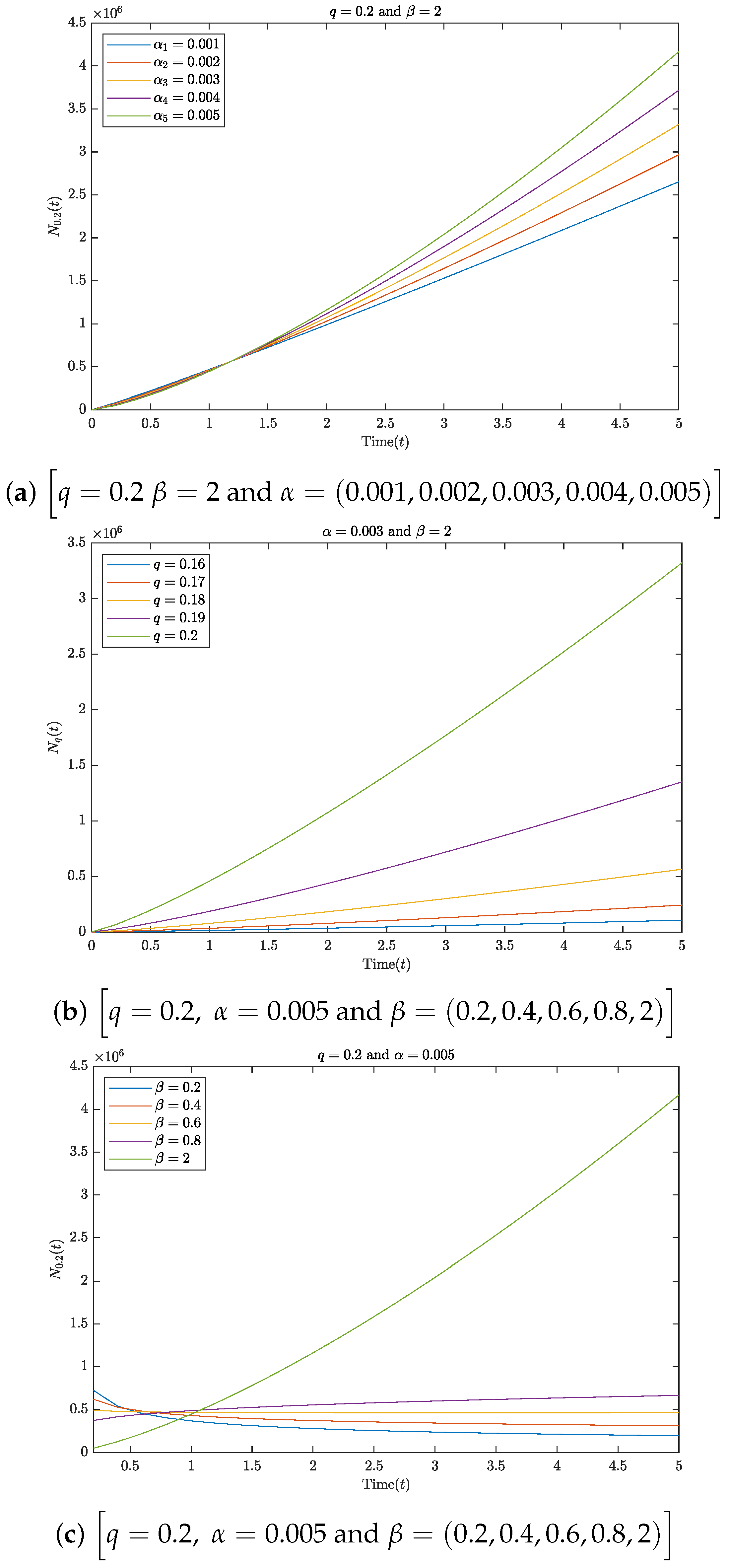
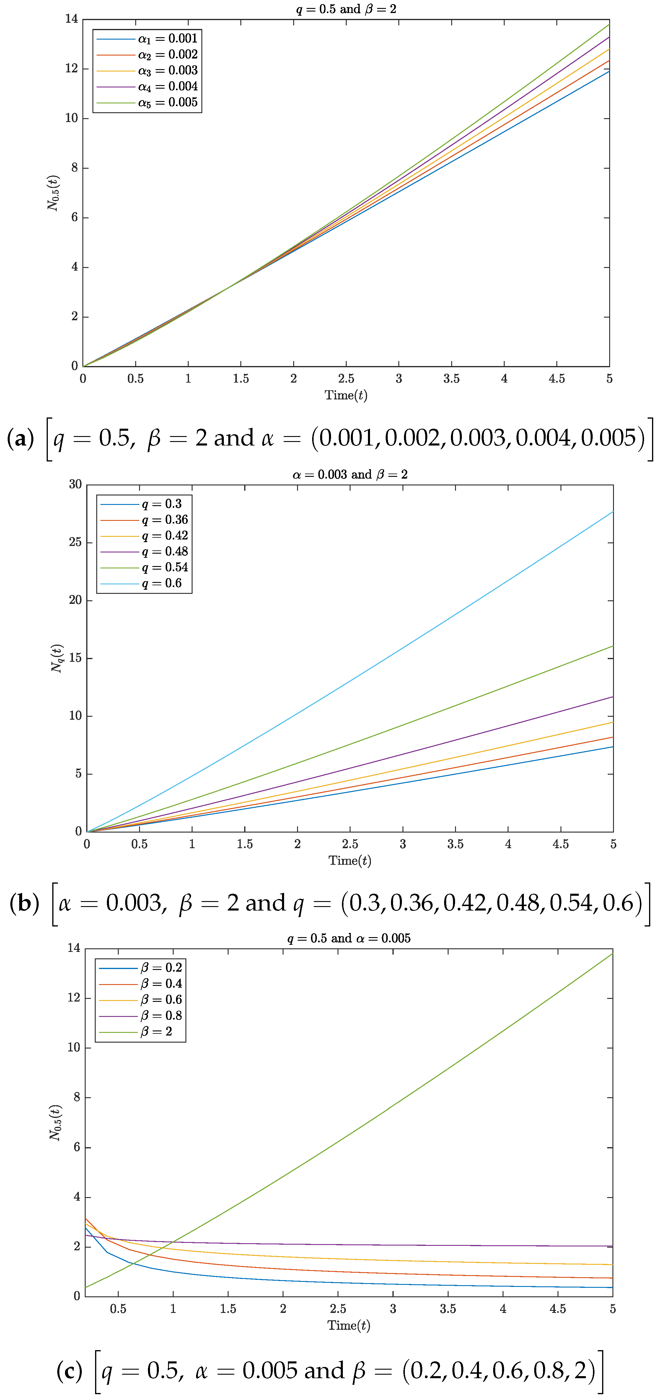
6. Graphical Representations

In this section, we offer a graphical elucidation of the determined results with different values for the parameters in Equations (71) and (73). Figure 1 and Figure 2 are the visual representations of Equations (71) and (73), respectively, using the parameters  N 0 = 1 , c = 1 , t [ 0 , 5 ] , and  λ = δ . In Figure 1a and Figure 2a, we fix the values of q and  β and drew graphs for different values of  α . In Figure 1b and Figure 2b, we set the values of  α and q and drew plots for different values of  β . In Figure 1c and Figure 2c, we fixed the values of  α and  β and drew graphs for different q values. All the different values for the parameters were chosen according to the conditions of convergence of the functions in Equations (33) and (34). Furthermore, we could obtain several results from the graphical solutions to Equations (71) and (73) by selecting different values for  λ , δ , α , β , and q that satisfied convergence of the functions in Equations (33) and (34).

7. Conclusions

Motivated by the established applications and future applications of fractional analysis in many branches of science, as well as the advent of a significantly larger spectrum of generalized Mittag-Leffler functions in statistics [30], physics [7], engineering [8], and other fields [31], this manuscript presents new forms of generalized hyper q-Mittag-Leffler functions in Equations (33) and (34). Then, we provided some of the convergence properties, fractional q-derivative, and q-integral operators of these functions. Furthermore, we investigated the solutions to the q-fractional kinetic equations in terms of the decided generalized hyper q-Mittag-Leffler functions by applying the defined q-Sumudu transform. Also, some exceptional cases for our principal outcomes were archived. In addition, we introduced graphical representations of the solutions, demonstrated in Section 5, using the program MATLAB.

Author Contributions

Methodology, M.A. (Mohamed Akel) and M.Z.A.; investigation, M.Z.A. and M.A. (Mohamed Abdalla); writing—original draft, M.A. (Mohamed Akel), M.Z.A., and M.A. (Mohamed Abdalla); writing—review and editing, M.A. (Mohamed Akel), M.Z.A., and M.A. (Mohamed Abdalla); supervision, M.A. (Mohamed Abdalla). All authors have read and agreed to the published version of the manuscript.

Funding

This work was funded by the Deanship of Scientific Research at King Khalid University through a large group research project under grant number RGP2/432/44.

Data Availability Statement

No data were used to support this study.

Conflicts of Interest

The authors declare that they have no conflicts of interest.

References

  1. Noeiaghdam, S.; Sidorov, D. Caputo-Fabrizio fractional derivative to solve the fractional model of energy supply demand system. Math. Model. Eng. Probl. 2020, 7, 359–367. [Google Scholar] [CrossRef]
  2. Fallahgoul, H.A.; Focardi, S.M.; Fabozzi, F.J. Fractional Calculus and Fractional Processes with Applications to Financial Economics, Theory and Application; Elsevier/Academic Press: London, UK, 2017. [Google Scholar]
  3. Benson, D.A.; Meerschaert, M.M.; Revielle, J. Fractional calculus in hydrologic modeling: A numerical perspective. Adv. Water Resour. 2013, 51, 479–497. [Google Scholar] [CrossRef] [PubMed]
  4. Ali, M.F.; Sharma, M.; Jain, R. An application of fractional calculus in electrical engineering. Adv. Eng. Tec. Appl. 2016, 5, 41–45. [Google Scholar] [CrossRef]
  5. Ghanbari, B.; Günerhan, H.; Srivastava, H.M. An application of the Atangana-Baleanu fractional derivative in mathematical biology: A three-species predator-prey model. Chaos Solitons Fractals 2020, 138, 109910. [Google Scholar] [CrossRef]
  6. Mishra, S.; Mishra, L.N.; Mishra, R.K.; Patnaik, S. Some applications of fractional calculus in technological development. J. Fract Calc. Appl. 2019, 10, 228–235. [Google Scholar]
  7. Jacob, J.S.; Priya, J.H.; Karthika, A. Applications of fractional calculus in science and engineering. J. Critical. Rev. 2020, 7, 4385–4394. [Google Scholar]
  8. Sabatier, J.; Agrawal, O.P.; Tenreiromachado, J.A. Advances in Fractional Calculus. Theoretical Developments and Applications in Physics and Engineering; Springer: Berlin/Heidelberg, Germany, 2007. [Google Scholar]
  9. Agarwal, P.; Chand, M.; Baleanu, D.; Regan, D.O.; Jain, S. On the solutions of certain fractional kinetic equations involving k-Mittag-Leffler function. Adv. Differ. Equ. 2018, 2018, 249. [Google Scholar] [CrossRef]
  10. Saxena, R.K.; Kalla, S.L. On the solutions of certain fractional kinetic equations. Appl. Math. Comput. 2008, 199, 504–511. [Google Scholar] [CrossRef]
  11. Akel, M.; Hidan, M.; Boulaaras, S.; Abdalla, M. On the solutions of certain fractional kinetic matrix equations involving Hadamard fractional integrals. AIMS Math. 2022, 7, 15520–15531. [Google Scholar] [CrossRef]
  12. Hidan, M.; Akel, M.; Abd-Elmageed, H.; Abdalla, M. Some matrix families of the Hurwitz-Lerch ζ-functions and associted for fractional kinetic equations. Fractals 2022, 30, 2240199. [Google Scholar] [CrossRef]
  13. Almalkia, Y.; Abdalla, M. Analytic solutions to the fractional kinetic equation involving the generalized Mittag-Leffler function using the degenerate Laplace type integral approach. Eur. Phys. J. Spec. Top. 2023, 232, 2587–2593. [Google Scholar] [CrossRef]
  14. Kolokoltsov, V.N.; Troeva, M. A new approach to fractional kinetic evolutions. Fractal Fract. 2022, 6, 49. [Google Scholar] [CrossRef]
  15. Habenom, H.; Oli, A.; Suthar, D.L. (p, q)-Extended Struve function: Fractional integrations and application to fractional kinetic equations. J. Math. 2021, 2021, 5536817. [Google Scholar] [CrossRef]
  16. Abdalla, M.; Akel, M. Contribution of using Hadamard fractional integral operator via Mellin integral transform for solving certain fractional kinetic matrix equations. Fractal Fract. 2022, 6, 305. [Google Scholar] [CrossRef]
  17. Garg, M.; Chanchlani, L. On fractional q-kinetic equation. Mat. Bilt. 2012, 36, 33–46. [Google Scholar] [CrossRef]
  18. Purohit, S.D.; Ucar, F. An application of q-Sumudu transform for fractional q-kinetic equation. Turk. J. Math. 2018, 42, 726–734. [Google Scholar] [CrossRef]
  19. Bairwa, R.K.; Kumar, A.; Kumar, D. Certain properties of generalized q-Mittag-Leffler type function and its application in fractional q-kinetic equation. Int. J. Appl. Comput. Math. 2022, 219, 22–31. [Google Scholar] [CrossRef]
  20. Abujarad, E.; Jarad, F.; Abujarad, M.H.; Baleanu, D. Application of q-Shehu transform on q-fractional kinetic equation involving the generalized hyper-Bessel function. Fractals 2022, 30, 2240179. [Google Scholar] [CrossRef]
  21. Annaby, M.H.; Mansour, Z.S. q-Fractional Calculus and Equations; Springer: Berlin/Heidelberg, Germany, 2012. [Google Scholar]
  22. Aral, A.; Gupta, V.; Agarwal, R.P. Applications of q-Calculus in Operator Theory; Springer: New York, NY, USA; Berlin/Heidelberg, Germany; Dordrecht, The Netherlands; London, UK, 2013. [Google Scholar]
  23. Chakraverty, S.; Jena, R.M.; Jena, S.K. Computational Fractional Dynamical Systems: Fractional Differential Equations and Applications; John Wiley and Sons, Inc.: Hoboken, NJ, USA, 2023. [Google Scholar]
  24. Gasper, G.; Rahman, M.; George, G. Basic Hypergeometric Series; Cambridge University Press: Cambridge, UK, 2004; Volume 96. [Google Scholar]
  25. Mansour, M. An asymptotic expansion of the q-Gamma function Γq(x). J. Nonlinear Math. Phys. 2006, 13, 479–483. [Google Scholar] [CrossRef]
  26. Mittag-Leffler, G. Sur la nouvelle fonction Eα(x). C. R. Acad. Sci. 1903, 137, 554–558. [Google Scholar]
  27. Wiman, A. Über de fundamental satz in der theoric der funktionen Eα(x). Acta Math. 1905, 29, 191–201. [Google Scholar] [CrossRef]
  28. Prabhakar, T.R. A singular integral equation with a generalized Mittag-Leffler function in the Kernel. Yokohama Math. J. 1971, 19, 7–15. [Google Scholar]
  29. Shukla, A.K.; Prajapati, J.C. On a generalization of Mittag-Leffler function and its properties. J. Math. Anal. Appl. 2007, 336, 797–811. [Google Scholar] [CrossRef]
  30. Gorenflo, R.; Kilbas, A.A.; Mainardi, F.; Rogosin, S. Mittag-Leffler Functions, Related Topics and Applications, 2nd ed.; Springer: Berlin/Heidelberg, Germany, 2020. [Google Scholar]
  31. Kumar, D.; Ram, J.; Cho, J. Dirichlet averages of deneralized Mittag-Leffler type function. Fractal Fract. 2022, 6, 297. [Google Scholar] [CrossRef]
  32. Jain, A. Generalization of Mittag-Leffler function and it’s application in quantum-calculus. Int. J. Innov. Res. Technol. Manag. 2018, 2, 1–4. [Google Scholar]
  33. Mansour, Z.S.I. Linear sequential q-difference equations of fractional order. Fract. Calc. Appl. Anal. 2009, 12, 159–178. [Google Scholar]
  34. Sharma, S.K.; Jain, R. On some properties of generalized q-Mittag Leffler function. Math. Aterna. 2014, 4, 613–619. [Google Scholar]
  35. Purohit, S.D.; Kalla, S.L. A generalization of q-Mittag-Leffler function. Mat. Bilt. 2011, 35, 15–26. [Google Scholar]
  36. Aziza, S.; Ahmada, K.; Khanb, B.; Sallehc, Z.; Alia, S.; Bilala, H.; Khand, M.G. Applications of q-Mittag-Leffler type Poisson distribution to subclass of q-starlike functions. J. Math. Comput. Sci. 2023, 29, 272–282. [Google Scholar] [CrossRef]
  37. Rajković, P.M.; Marinkovixcx, S.D.; Stankovixcx, M.S. On q-analogues of Caputo derivative and Mittag-Leffler function. Fract. Calc. Appl. Anal. 2007, 10, 359–374. [Google Scholar]
  38. Garg, M.; Chanchlani, L.; Kalla, S. A q-analogue of generalized Mittag-Leffler function. Algebr. Group Geometr. 2011, 28, 205–223. [Google Scholar]
  39. Nadeem, R.; Usman, T.; Nisar, K.S.; Abdeljawad, T. A new generalization of Mittag-Leffler function via q-calculus. Adv. Differ. Equ. 2020, 2020, 695. [Google Scholar] [CrossRef]
Figure 1. Plot of Equation (71) for  N 0 = 1 , c = 1 , t [ 0 , 5 ] .
Fractalfract 08 00058 g001
Figure 2. Plot of Equation (73) for  N 0 = 1 , c = 1 , t [ 0 , 5 ] .
Fractalfract 08 00058 g002
Disclaimer/Publisher’s Note: The statements, opinions and data contained in all publications are solely those of the individual author(s) and contributor(s) and not of MDPI and/or the editor(s). MDPI and/or the editor(s) disclaim responsibility for any injury to people or property resulting from any ideas, methods, instructions or products referred to in the content.

