Article

Multistability Mechanisms for Improving the Performance of a Piezoelectric Energy Harvester with Geometric Nonlinearities

School of Mechanical Engineering, Shanghai Institute of Technology, Shanghai 201418, China
*
Author to whom correspondence should be addressed.
Fractal Fract. 2024, 8(1), 41; https://doi.org/10.3390/fractalfract8010041
Submission received: 6 December 2023 / Revised: 29 December 2023 / Accepted: 6 January 2024 / Published: 8 January 2024

Abstract

:
This study presents multistability mechanisms that can enhance the energy harvesting performance of a piezoelectric energy harvester (PEH) with geometrical nonlinearities. To configure triple potential wells, static bifurcation diagrams in the structural parameter plane are depicted. On this basis, the key structural parameter is considered, of which three reasonable values are then chosen for comparing and evaluating the performances of the triple-well PEH under them. Then, intra-well responses and the corresponding voltages of the system are investigated qualitatively. A preliminary analysis of the suitable energy-harvesting conditions is carried out, which is then validated by numerical simulations of the evolution of coexisting attractors and their basins of attraction with variations in the excitation level and frequency. It follows that, under a low-level ambient excitation, the intra-well responses around the trivial equilibrium dominate the energy-harvesting performance. When the level of the environmental excitation is very low, which one of the three values of the key structural parameter is the best for improving the performance of the PEH system depends on the range of the excitation frequency; when the excitation level increases sufficiently to induce inter-well responses, the maximum one is the best for improving the performance of the PEH. The findings provide valuable insights for researchers working in the structure optimization and practical applications of geometrically nonlinear PEHs.

1. Introduction

In recent years, energy harvesting has gained significant attention as a sustainable solution for powering electronic devices [1,2,3]. Piezoelectric conversion is one of the most widely used methods of energy conversion for energy harvesters as it is convenient for the configuration of the devices, specifically the ones immune to electromagnetic interference [4]. To construct piezoelectric energy harvesters (PEHs), linear cantilever beams were first taken into account due to the simplicity of their structures. Actually, this type of piezoelectric energy harvester can achieve a good energy-harvesting performance only if the ambient excitation frequency is close to the natural frequency of the beam, showing that its bandwidth for the high efficiency of energy collection is extremely narrow [5]. Later, the multi-array linear cantilever beams were introduced to the design of the primary structures of PEHs. Although the multi-array linear-beam PEHs have a broader useful bandwidth, the density of their harvested power is still low [6].
To tackle this problem, nonlinear stiffness was added to the configuration of PEHs because nonlinear factors in the oscillating systems of PEHs could be beneficial for both broadening the useful bandwidth of energy collection and increasing the energy harvesting efficiency [7,8,9]. For instance, to configure a nonlinear mono-beam PEH, a small magnetic mass is usually attached to the free end of the beam, and several small eternal magnets are attached to the base nearby, which could lead to nonlinear magnetic coupling forces [10,11,12,13]. As a result, its bandwidth for high-efficiency energy harvesting could be broadened due to the stiffness softening effect of its oscillatory system. The research of this type of PEH has attracted much attention in recent years. According to their experimental results, Fan et al. [14] illustrated that, compared with the cantilever-beam PEH without magnets, the one with magnets could present a wider bandwidth and a much higher power output by adjusting the gap between the tip mass and the external magnet. Via numerical simulations and experiments, Zhao and Erturk [15] also found that PEHs with bistability characteristics could collect more kinetic energy than the monostable ones, specifically at a low excitation level. Wang et al. [16] utilized elastic amplifiers to further increase the output of bistable PEHs. The tristable configuration can also be achieved by varying the distance between the two external magnets on the base. In the literature, it is explained that this configuration of PEHs is more advantageous than the double-well configuration for vibration energy harvesting [17,18,19,20], because the potential barrier is lower in the former than in the latter.
Apart from magnet-mass-beam PEHs, the configuration of obliquely set-up springs in the spring-mass PEHs can also lead to stiffness nonlinearities, in other words, geometrical nonlinearities [21]. For example, as a typical geometric nonlinear oscillator, the smooth and discontinuous (SD) oscillator composed of a lumped mass and two inclined springs has two potential wells and exhibits the coexistence of multiple stable responses and jumps among them [22]; thus, it is usually applied to construct the primary structures of PEHs. To date, there have been a number of studies on the design and mechanisms of geometrically nonlinear PEHs. Ramlan et al. [23] explored the potential benefits of geometrically nonlinear stiffness in energy-harvesting devices via numerical simulations and found that a bistable snap-through mechanism could be employed to expand the displacement of the oscillator as well as to harvest more energy even if the excitation frequency was significantly lower than its natural frequency. Taking the effect of the Gaussian white noise of the environment into consideration, the phenomenon snap-through was also found to be easily triggered by the geometrically nonlinear configuration of PEHs [24,25]. To harvest wave energy, Younesian and Alam [26] proposed a PEH whose primary structure consisted of a rod and two symmetrical springs. The quantitative investigation demonstrated that, compared to the PEH with a traditional linear spring connected directly to a buoy, the wave energy-harvesting efficiency of the proposed PEH was noticeably higher. Based upon the SD oscillator, Yang and Cao [27,28] proposed a tristable PEH whose stiffness and resonant frequency could be adjusted by the variation in a structural parameter; thus, it could achieve a broader useful bandwidth and a higher average power output than monostable and bistable PEHs.
Nevertheless, when evaluating the work performance of PEHs, the influence of the initial conditions on the PEH systems has seldom been discussed. In fact, under the circumstances of multistability, one can hardly determine the final dynamics as well as the power output of the PEH oscillatory systems without taking the disturbance to their initial states into account. For instance, the qualitative analysis of the PEHs has been used to illustrate the large-amplitude inter-well resonant responses that correspond to much higher voltage outputs coexisting with the intra-well ones, which correspond to lower voltage outputs [29,30]. This cannot warrant a better working performance of the PEHs as achieving the inter-well responses remains a challenge when the initial states are perturbed around the equilibria of the PEH oscillatory systems.
Based on the above statement, we investigate the mechanisms of the performance improvement of a geometrically nonlinear tristable PEH by discussing the couple effect of the ambient excitation, its structural parameters, and initial conditions. The rest of the paper is organized as follows: In Section 2, the PEH oscillatory system and its nondimensional system is derived, and the values of some structural parameters are determined based upon its static bifurcations; in Section 3, in the case of three potential wells, the intra-well resonant responses and the corresponding voltage outputs of the nondimensional system are analyzed; Section 4 presents the numerical results of the coexisting responses and their basins of attraction in order to both validate the qualitative prediction and determine the value of a structural parameter to achieve the best performance of the PEH; finally, some novel findings are summarized in Section 5.

2. Dynamical Model and Unperturbed Dynamics

2.1. Oscillatory System of the PEH and Its Nondimensional System

A top view of a geometrically nonlinear PEH is shown in Figure 1. In the primary structure of this PEH, the mass block M is attached to the piezoelectric stack and connected to one vertical spring of the stiffness coefficient K v and four inclined springs whose stiffness coefficients are all K h . Without excitation, the vertical spring remains undeformed, and the four obliquely set-up springs are arranged symmetrically about the centroid of the lumped mass. When the structure is subjected to the external excitation Y, the corresponding displacement of the mass is X . And the piezoelectric stack will be under pressure and deformed, resulting in the generation of a current. Based on Newton’s second law and Kirchhoff’s law, the oscillatory system of the PEH can be expressed as the following ordinary differential equation [31]:
M X ¨ + C X ˙ + K v X + 2 K h ( X + c ) ( 1 L ( X + c ) 2 + d 2 ) + 2 K h ( X c ) ( 1 L ( X c ) 2 + d 2 ) + β 1 V = M Y ¨ , β 2 X ˙ = C p V ˙ + V R p .
The physical meanings of the parameters in the above equation are provided in Table 1. For the environmental excitation applied to the base, we assumed it was harmonic, expressed by
Y = F cos Ω T .
For the simplicity of the analysis, we set
x = X L , y = Y L , v = V V 0 , ω 1 2 = K v M , T = ω 1 t , (   ) = d (   ) d T , c ^ = c L , d ^ = d L , r = 2 K h K v , ξ = C M ω 1 , η = β 1 V 0 K v L , δ = 1 C p R P ω 1 , γ = β 2 L C p V 0 , f 0 = M F Ω 2 K v , ω = Ω ω 1 .
and rewrite system (1) as the nondimensional system below:
x ¨ + ξ x ˙ + ( 2 r + 1 ) x r ( x + c ^ ( x + c ^ ) 2 + d ^ 2 + x c ^ ( x c ^ ) 2 + d ^ 2 ) + η v = f 0 cos ω T , γ x ˙ = v ˙ + δ v .
The number of the parameters in the nondimensional system is noticeably lower than that of the parameters in the original system (1).

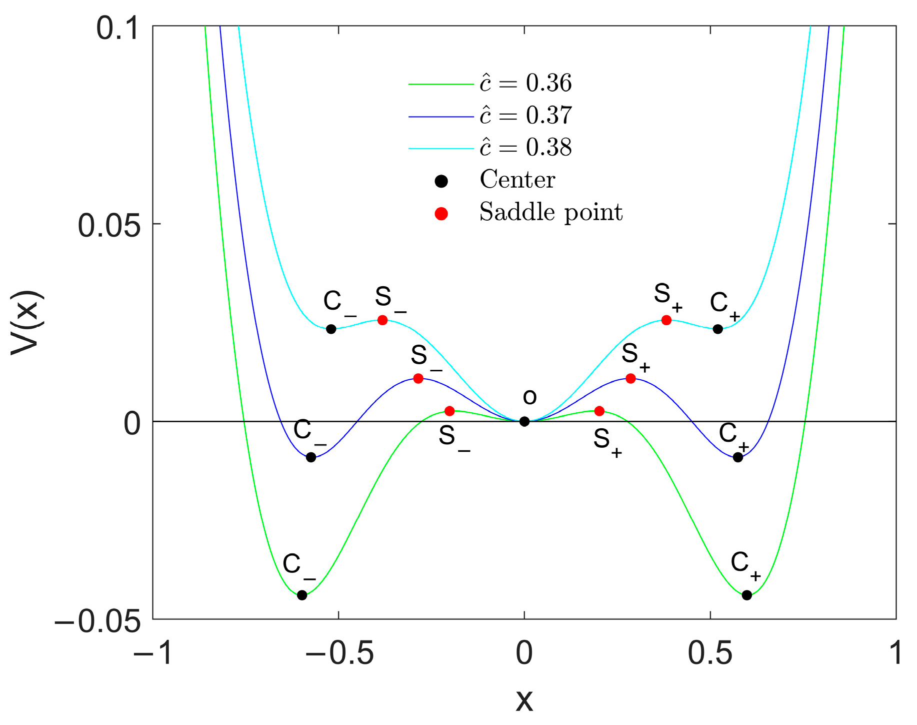
2.2. Static Bifurcations and Structural Parameters to Configure Triple Wells

Since the electric system has a very weak effect on the oscillation of the primary structure, the unperturbed system of the nondimensional system (3) can be expressed as the unperturbed system of the oscillator, i.e.,
x ˙ = y , y ˙ = ( 2 r + 1 ) x + r ( x + c ^ ( x + c ^ ) 2 + d ^ 2 + x c ^ ( x c ^ ) 2 + d ^ 2 ) .
It is a Hamilton system with the following Hamiltonian H(x, y) and potential energy V(x):
H ( x , y ) = 1 2 y 2 + ( 1 2 + r ) x 2 r ( ( x + c ^ ) 2 + d ^ 2 + ( x c ^ ) 2 + d ^ 2 ) + 2 r c ^ 2 + d ^ 2 , V ( x ) = ( 1 2 + r ) x 2 r ( ( x + c ^ ) 2 + d ^ 2 + ( x c ^ ) 2 + d ^ 2 ) + 2 r c ^ 2 + d ^ 2 .
By letting the right side of Equation (5) be zero, one can determine its equilibria. Obviously, the vertical coordinates y for the equilibria are all zero, and their horizontal coordinates x can be solved from the irrationally nonlinear equation below:
( 2 + 1 r ) x ( x + c ^ ( x + c ^ ) 2 + d ^ 2 + x c ^ ( x c ^ ) 2 + d ^ 2 ) = 0 .
The stability of the equilibria can be determined by the roots of the following characteristic equation:
λ 2 + ( 2 r + 1 ) r d ^ 2 ( 1 ( ( x + c ^ ) 2 + d ^ 2 ) 3 / 2 + 1 ( ( x c ^ ) 2 + d ^ 2 ) 3 / 2 ) = 0 .
Accordingly, the number, positions, and the stability of the equilibria are decided by the values of the three dimensionless parameters r ,   c ^ , and d ^ . Their related original parameters are the stiffness coefficients K h and K v as well as the distances c and d. As it can be seen in Figure 1, it is very convenient to adjust the half distance between the two pins c with the aid of the slideways on both sides of the frame.
To obtain the horizontal coordinates of the equilibria, we need to solve Equation (7). Obviously, there are two fractional and irrationally nonlinear terms in it. By identical transformations, Equation (7) can become a polynomial in the form of ( C 1 x 10 + C 2 x 8 + C 3 x 6 + C 4 x 4 + C 5 x 2 + C 6 ) x 2 = 0 . According to Abel’s theorem, it is hard for us to express the solutions in the explicit functions of r ,   c ^ , and d ^ . Even if the fractional terms were approximately expanded as fifth-order polynomials, the error would still be large to determine the conditions for static bifurcations [31]. To deal with this issue, we adopted the cell mapping method to depict the static bifurcation diagrams numerically in the parameter plane c ^ d ^ , which comprises the 499 × 499 arrays of parameter condition points in the ranges of 0 < c ^ < 1 and 0 < d ^ < 1 .
At different values of r , the details for the static bifurcation diagrams of the unperturbed system (5) and the corresponding phase portraits are described in Figure 2. In this case, the colors red, yellow, and green denote different regions. For the parameters c ^ and d ^ chosen in the same region, the numbers of equilibria and the nature of the potential wells are the same. In each subfigure, we can observe the cases of mono-, double, and triple potential wells. Since 0.5 is a practical value for the parameter d ^ [27], we added a dashed line in each subfigure for it. It is evident in Figure 2 that, as r increases, the parameter regions for the cases of multiple potential wells are enlarged. It means that, with the increase in r, the PEH may have more possibilities to gain tristable characteristics, which is beneficial for the performance improvement of the device. Nevertheless, in practical applications, it is suggested to avoid an excessively large stiffness ratio of K h to K v , i.e., a large value of r. Considering the area of the multiple potential well regions at r = 5 and r = 9 is similar (see Figure 2b,c), we chose to set r = 5 in the subsequent research. Without the loss of practical significance, we set the following values for the parameters of system (4) to configure the triple potential wells [27]:
r = 5 ,   d ^ = 0.5 ,   ξ = 0.01 ,   η = 0.2 ,   γ = 0.3 ,   δ = 0.1 .
In Figure 2b, there is a small interval of c ^ for the case of triple potential wells. To compare the performances of the PEH for different values of c ^ , we chose three values of c ^ in the interval (see the dashed line in the green region of Figure 2b), namely, 0.36, 0.37, and 0.38. Considering the original length of the spring L = 10 cm and c ^ = c / L , the variation in the parameter c ^ from 0.36 to 0.37 or from 0.37 to 0.38 means the vertical half distance between two pins c increases by 1 mm. By sliding the pins along the slideways of both sides of the frame (see Figure 1), it is very easy to achieve the variation in the distance.
The unperturbed orbits for these three values of c ^ are illustrated in Figure 3. Apparently, there are three potential wells in each subfigure. With the increase in c ^ , the area of the potential well around the origin O ( 0 , 0 ) expands, while the area of the potential wells around the nontrivial equilibria C ± ( ± x c , 0 ) shrinks. In systems (1) and (2), the three potential well centers mean the stable equilibrium positions. In other words, without excitation, the mass block of the PEH remains at one of the three positions and the voltage output is zero.
In the unperturbed system (6), the variation in the potential energy with the displacement x can be observed in Figure 4. Evidently, for different values of c ^ or different potential wells, the potential energy differences between the potential well centers and the saddle points nearby are totally different. For instance, among all the potential energy differences, the one between the nontrivial center C + and the saddle point S + at c ^ = 0.38 is the lowest, indicating that the energy to escape from this potential well is the lowest. Similarly, to escape from the potential well around the center O(0, 0), the energy consumed at c ^ = 0.36 is the lowest. The potential energy differences were calculated, as shown in Table 2. Since the escape of orbits from a potential well surrounded by homoclinic orbits means a homoclinic bifurcation, which usually leads to a larger displacement inter-well response corresponding to a higher power output of the PEH, the value of the structural parameter c ^ chosen at 0.38 is the best for energy harvesting when the excitation level is high enough to trigger the global bifurcation. At a lower ambient excitation level, this is not necessarily the case, as the performance of the PEH depends on the amplitude of the intra-well resonant responses rather than the inter-well ones. The corresponding investigation is presented in the next section.

3. Intra-Well Resonant Responses and the Corresponding Voltages

In the case of triple potential wells, there are responses in the vicinity of the three centers when the excitation is weak. Since the vibration energy harvesting of the PEH can be more effective when the primary resonance occurs, we focused on the intra-well resonant responses and the corresponding voltages. The analytical method we applied was the method of multiple scales (MMS). The numerical simulations using the fourth-order Runge–Kutta approach were then conducted to validate the analysis.

3.1. Resonant Solutions near the Trivial Center O(0, 0)

To apply the MMS for the intra-well resonant responses, we first rescaled the dimensionless parameters ξ , η , δ , and f 0 . Considering the small damping, the weak effect of the electric circuit on the oscillation of the primary structure, the high piezoelectric capacitance, and the low excitation level in the original system (1), the values of the dimensionless parameters ξ , η , δ , and f 0 are small. Using the new small parameter ε, they are rescaled as follows:
ξ = ε ξ ˜ , η = ε η ˜ , δ = ε δ ˜ , f 0 = ε 2 f ˜ .
The nondimensional system (4) becomes
x ¨ + ε ξ ˜ x ˙ + ( 2 r + 1 ) x r ( x + c ^ ( x + c ^ ) 2 + d ^ 2 + x c ^ ( x c ^ ) 2 + d ^ 2 ) + ε η ˜ v = ε 2 f ˜ cos ω T , γ x ˙ = v ˙ + ε δ ˜ v .
Next, by expanding the fractional terms of the above system in the Taylor series of x in the neighborhood of x = 0, and neglecting higher-order-than-three terms of x, we rewrite Equation (11) as
x ¨ + ω ˜ 2 x = ε ξ ˜ x ˙ + k 3 x 3 ε η ˜ v + ε 2 f ˜ cos ω T , γ x ˙ = v ˙ + ε δ ˜ v , ,
where
ω ˜ = 1 + 2 r 2 r d ^ 2 ( c ^ 2 + d ^ 2 ) 3 / 2 ,   k 3 = ( 4 c ^ 2 d ^ 2 d ^ 4 ) ( c ^ 2 + d ^ 2 ) 7 / 2 r .
In the above equation, the parameter ω ˜ denotes the resonant frequency of this mode. At different values of the structural parameter c ^ , the values of ω ˜ can be calculated, as it can be seen in Table 3. Among the three values of ω ˜ at the three values of c ^ , ω ˜ at c ^ = 0.36 is the lowest. This implies that, in the case of a very low ambient excitation frequency, the PEH system at c ^ = 0.36 has the highest possibility of achieving the resonant response, thus harvesting more vibration energy.
Considering system (12) under the primary resonance, we rescale the dimensionless excitation frequency ω as
ω = ω ˜ + ε σ ,
Then, by introducing time scales and differential operators, we rescale the dimensionless displacement x and the time differentials in system (12) as below:
x = i = 1 n ε i x i ( T 0 , T 1 , T 2 , ) ,   v = i = 1 n ε i v i ( T 0 , T 1 , T 2 , ) ,   T i = ε i T ,   d d T = i = 0 n ε i D i ,   D i = T i .
By comparing the coefficients of ε , ε 2 , and ε 3 of system (12), we have
ε 1 : D 0 2 x 1 + ω 2 x 1 = 0 ,     D 0 v 1 = γ D 0 x 1 ,
ε 2 : D 0 2 x 2 + ω 2 x 2 = 2 D 0 D 1 x 1 ξ ˜ D 0 x 1 + 2 σ ω x 1 + f ˜ cos ω T η ˜ v 1 ,     D 0 v 2 = γ D 0 x 2 + γ D 1 x 1 D 1 v 1 δ ˜ v 1 ,
and
ε 3 : D 0 2 x 3 + ω 2 x 3 = 2 D 0 D 1 x 2 ( D 1 2 + 2 D 0 D 2 ) x 1 ξ ˜ ( D 0 x 2 + D 1 x 1 ) + 2 σ ω x 2 η ˜ v 2 + k 3 x 1 3 σ 2 x 1 ,
respectively.
The general solution of Equation (16) can be obtained as
x 1 = A ( T 1 , T 2 ) e i ω T 0 + A ¯ ( T 1 , T 2 ) e i ω T 0 , v 1 = γ A e i ω T 0 + γ A ¯ e i ω T 0
where
A ( T 1 , T 2 ) = a ( T 1 , T 2 ) 2 e i φ ( T 1 , T 2 ) .
where a ( T 1 , T 2 ) represents the amplitude of the solution x 1 and φ ( T 1 , T 2 ) is the phase difference. Substituting Equations (19) and (20) into Equation (17) and eliminating its secular terms yield
D 1 A = f ˜ i 4 ω σ A i + η ˜ γ A i 2 ω 1 2 ξ ˜ A .
The solution of Equation (17) is then solved, expressed by
x 2 = 0 ,   v 2 = δ ˜ γ A i ω e i ω T 0 + c c .
Thereafter, by substituting Equations (19)–(22) into Equation (18) and eliminating the secular terms there, we obtain
D 2 A = 3 i A 2 A ¯ k 3 2 ω i σ f ˜ 8 ω 2 A δ ˜ γ η ˜ 2 ω 2 + i A γ σ η ˜ 2 ω 2 + i γ f ˜ η ˜ 16 ω 3 i A γ 2 η ˜ 2 8 ω 3 + f ˜ ξ ˜ 16 ω 2 i A ξ ˜ 2 8 ω .
Based on Equations (15), (19), and (22), the resonant solution in the vicinity of the origin can be expressed as
x = a ^ cos ( ω T + φ ) ,   v = ( γ a ^ ) sin ( ω T + φ arcsin ( 2 ω 4 ω 2 + δ 2 ) ) ,
where the response amplitude a ^ is expressed by
a ^ = ε a .
Substituting Equations (20), (21), and (23) into the following equation
A ˙ D 0 A + ε D 1 A + ε 2 D 2 A ,
and returning the parameters to the dimensionless parameters of the nondimensional system (4) yield the following differential equation about a ^ and φ :
a ^ ˙ = ω ( γ η δ + ξ ω 2 ) a ^ 2 ω 3 + ( γ η + 2 ω ( 3 ω + ω ˜ ) ) f 0 sin φ + ξ ω f 0 cos φ 8 ω 3 , a ^ φ ˙ = a ^ ( γ 2 η 2 + ω 2 ( ξ 2 + 3 k 3 a ^ 2 + 8 ω ( ω ω ˜ ) ) + 4 γ η ω ( 2 ω + ω ˜ ) ) 8 ω 3 + ( γ η + 2 ω ( 3 ω + ω ˜ ) ) f 0 cos φ ξ ω f 0 sin φ 8 ω 3 .
By letting a ^ ˙ = 0 and φ ˙ = 0 , we can solve the amplitude and phase difference of the periodic solution using the equation below:
4 ω ( γ η δ + ξ ω 2 ) a ^ = ( γ η + 2 ω ( ω ˜ 3 ω ) ) f 0 sin φ + ξ ω f 0 cos φ , a ^ ( γ 2 η 2 + ω 2 ( ξ 2 + 3 k 3 a ^ 2 + 8 ω ( ω ω ˜ ) ) + 4 γ η ω ( 2 ω + ω ˜ ) ) = ( γ η + 2 ω ( ω ˜ 3 ω ) ) f 0 cos φ ξ ω f 0 sin φ .
Eliminating the triangulation functions of the above equation yields
ξ 2 f 0 2 64 ω 4 + ( γ η f 0 8 ω 3 f 0 2 ω ( ω ω ˜ ) f 0 4 ω 2 ) 2 = ( ξ 2 + γ η δ 2 ω 2 ) 2 a ^ 2 + a ^ 2 ( 3 k 3 a ^ 2 8 ω + γ 2 η 2 + ω 2 ( ξ 2 + 8 ω ( ω ω ˜ ) ) + 4 γ η ω ( ω ˜ 2 ω ) 8 ω 3 ) 2 .
The amplitude of the resonant solution x can be solved using Equation (29). As shown in Equation (24), the amplitude of the voltage under the primary resonance is γ a ^ . Since the coefficient γ is fixed, the voltage is proportional to a ^ . Hence, the power output of the PEH system can be obtained by the analysis of the amplitude a ^ .
Based on the Jacobi matrix of Equation (27):
J ( a ^ , φ ) = [ ξ 2 γ η λ 2 ω 2 a ^ C 1 8 ω 3 C 1 + 6 k 3 ω 2 a ^ 2 8 ω 3 a ^ ξ 2 γ η λ 2 ω 2 ]
where
C 1 = γ 2 η 2 + 4 ω ˜ ω ( γ η 2 ω 2 ) + ω 2 ( ξ 2 8 γ η + 8 ω 2 + 3 k 3 a ^ 2 ) ,
we obtain the corresponding characteristic equation:
λ 2 + ( ξ + γ η δ ω 2 ) λ + 1 4 ω 4 ( ω 2 ξ + γ η δ ) 2 + C 1 ( C 1 + 6 k 3 ω 2 a ^ 2 ) 64 ω 6 = 0 .
The stability of the solution x is determined by the eigenvalues solved using Equation (32). If one eigenvalue of the solution has a positive real part, the solution is unstable; otherwise, it is stable. Since all the dimensionless parameters in Equation (32) are real numbers, there is no purely imaginary solution. Accordingly, the stability switch of the periodic solution occurs when λ = 0 , meaning the saddle-node (SN) bifurcations of the periodic solution in the vicinity of the origin O(0, 0). Thereby, SN bifurcation points can be used to divide the stable and unstable branches.
At low excitation levels, the variation in the response amplitude with the increase in the dimensionless excitation frequency ω at the three values of c ^ is displayed in Figure 5. In this case, ω is supposed to be no more than 1 since the frequency of the ambient excitation is low in most cases. In Figure 5a,b, one can observe the hard-stiffness characteristics, SN bifurcation points, and the coexistence of bistable solution branches at each value of c ^ and very low excitation levels, such as f 0 = 0.003 and f 0 = 0.005 . The numerical results match the analytical ones well, validating the analysis. It follows from the comparison of Figure 5a,b that the response amplitude increases when the excitation level increases. Additionally, for different values of c ^ , the band of the excitation frequency for the coexistence of bistable responses is totally different. Observing the curves in each color, one may find that between the two SN bifurcation points, two stable solution branches coexist. The upper branch corresponds to a higher amplitude response, hence leading to a higher power output. From the comparison of the same-colored curves in Figure 5a,b, it is evident that the bandwidth of the coexistence of the two stable solution branches is broadened by the increase in the excitation level, meaning that, even at a low excitation frequency, the PEH system may have a high voltage output. Moreover, comparing the three different-colored curves in Figure 5a,b, it can be seen that the bandwidth of the bistable branches is the lowest at c ^ = 0.36 but the highest at c ^ = 0.38 . Therefore, the PEH oscillatory system (4) at c ^ = 0.36 has more of a chance to achieve a high amplitude response in the vicinity of the origin O(0, 0), thus harvesting more vibration energy when the ambient excitation is weak and of a low frequency.
On this basis, we compared the performance of the PEH system (4) at different values of the structural parameter c ^ at low excitation levels. Without the loss of fairness, we chose the excitation frequency in each frequency band of the bistable branches at c ^ = 0.36 , c ^ = 0.37 , and c ^ = 0.38 . Based upon supposing the low excitation frequency as ω = 0.5, ω = 0.7 and ω = 0.9 successively, the variation in the periodic responses around O(0, 0) with the increase in f0 is provided in Figure 6.
In Figure 6a, for each value of c ^ , there are two solid curves, and one is of a much higher amplitude than the other. It indicates that, at the three different values of c ^ , the upper response branches can also be achieved with the increase in the excitation amplitude. Among them, at c ^ = 0.36 , the system can obtain the upper response branch at the lowest ambient excitation level, while at c ^ = 0.38 , the amplitudes of the upper response branch are the highest. It suggests that, when ω = 0.5 and the excitation level is very low, 0.36 can be the most advantageous value for energy harvesting among the three values of the structural parameter c ^ , while for a higher excitation level, 0.38 is the best choice of c ^ .
As ω is increased to 0.7 (see Figure 6b), there is only one response branch for c ^ = 0.36 , as the excitation frequency is out of the frequency band for bistability. In contrast, there are still two stable solution branches for c ^ = 0.37 or c ^ = 0.38 . In this case, when the ambient excitation is weak, c ^ = 0.36 is still the best for energy harvesting because the response amplitudes on the only branch at c ^ = 0.36 are higher than the ones on the lower branches at c ^ = 0.37 and c ^ = 0.38 . Meanwhile, c ^ = 0.38 is the most beneficial when the excitation level is high enough to trigger bistability.
For ω = 0.9 (see Figure 6c), only at c ^ = 0.38 , there are two stable solution branches. If the excitation level is too low to trigger bistability at c ^ = 0.38 , 0.37 and 0.38 are both better choices for the structural parameter c ^ than 0.36, in consideration of efficient energy harvesting. Otherwise, 0.38 is the most useful among the three values of c ^ .

3.2. Resonant Solutions in the Vicinity of the Nontrivial Centers C ± ( ± x c , 0 )

To determine the periodic solutions near nontrivial centers C ± ( ± x c , 0 ) , similarly to the previous section, we also applied MMS. To begin with, we assumed the solutions perturbing the two centers, namely, x = ± x ^ + x c in Equation (10), thus yielding
x ^ ¨ + ε ξ ˜ x ^ ˙ ± ( 2 r + 1 ) x c + ( 2 r + 1 ) x ^ r ( x ^ + ( c ^ ± x c ) ( x ^ + ( c ^ ± x c ) ) 2 + d ^ 2 ) r ( x ^ ( c ^ x c ) ( x ^ ( c ^ x c ) ) 2 + d ^ 2 ) + ε η ˜ v = ε 2 f ˜ cos ω T .
Then, by expanding the fractional terms of the above system in the Taylor’s series of x ^ in the neighborhood of x ^ = 0 and neglecting the higher-order-than-three terms of x ^ , we have
x ^ ¨ + ω ^ 2 x ^ = ε ξ ˜ x ^ ˙ + ε 2 f ˜ cos ω T C 2 x ^ 2 C 3 x ^ 3 ε η ˜ v , γ x ^ ˙ = v ˙ + ε δ ˜ v ,
where
ω ^ = 1 + 2 r r d ^ 2 ( 1 ( d ^ 2 + ( c ^ + x c ) 2 ) 3 / 2 + 1 ( d ^ 2 + ( c ^ x c ) 2 ) 3 / 2 ) , C 2 = 3 d ^ 2 r 2 ( c ^ + x c ( d ^ 2 + ( c ^ + x c ) 2 ) 5 / 2 c ^ x c ( d ^ 2 + ( c ^ x c ) 2 ) 5 / 2 ) ,   C 3 = d ^ 2 r 2 ( d ^ 2 4 ( c ^ + x c ) 2 ( d ^ 2 + ( c ^ + x c ) 2 ) 7 / 2 + d ^ 2 4 ( c ^ x c ) 2 ( d ^ 2 + ( c ^ x c ) 2 ) 7 / 2 ) .
In this case, the resonant frequencies ω ^ at the three different values of c ^ are provided in Table 4. Obviously, ω ^ at c ^ = 0.38 is the lowest.
By rescaling the dimensionless excitation frequency ω , the displacement x ^ , and time scales of system (34) as
ω = ω ^ + ε σ ,   x ^ = i = 1 n ε i x ^ i ( T 0 , T 1 , T 2 , ) ,   v ^ = i = 1 n ε i v ^ i ( T 0 , T 1 , T 2 , ) ,
and applying MMS to the third order of ε again, we obtain the following approximate analytic form of the periodic solution near C ± ( ± x c , 0 ) :
x = ± x c + b ^ cos ( ω T + θ ) ,   v = b ^ γ ω 2 + δ 2 ω cos ( ω T + θ + arccos ( ω ω 2 + δ 2 ) ) ,
where the amplitude b ^ and phase angle θ satisfy
b ^ ˙ = ( ξ 2 γ η δ 2 ω 2 ) b ^ + ξ f 0 8 ω 2 cos θ + ( γ η f 0 8 ω 3 f 0 2 ω ( ω ω ^ ) f 0 4 ω 2 ) sin θ , b ^ θ ˙ = ( 4 γ η ξ 2 8 ω γ 2 η 2 8 ω 3 + ( γ η 2 ω 2 ) ( ω ω ^ ) 2 ω 2 ) b ^ + ( 3 C 3 8 ω 5 C 2 2 12 ω 3 ) b ^ 3 ξ f 0 8 ω 2 sin θ + ( γ η f 0 8 ω 3 f 0 2 ω ( ω ω ^ ) f 0 4 ω 2 ) cos θ .
According to Equation (37), the voltage amplitude is proportional to the response amplitude b ^ , indicating that, similarly to the previous section, the characteristics of the power output can be analyzed by discussing the intra-well periodic responses. For the steady-state periodic solutions in the vicinity of C ± , both b ^ ˙ and θ ˙ are zero, namely,
ξ f 0 ω cos θ + f 0 ( γ η 6 ω 2 + 2 ω ω ^ ) sin θ = 4 ω ( ω 2 ξ γ η δ ) b ^ , f 0 ( γ η 6 ω 2 + 2 ω ω ^ ) cos θ ξ f 0 ω sin θ = ( 10 3 C 2 2 3 ω 2 C 3 ) b ^ 3 + b ^ ( ( ξ 2 4 γ η ) ω 2 + γ 2 η 2 4 ω ( γ η 2 ω 2 ) ( ω ω ^ ) ) .
Eliminating the triangulation functions in the above equation yields
16 ω 2 ( ω 2 ξ γ η δ ) 2 b ^ 2 + [ ( 10 3 C 2 2 3 ω 2 C 3 ) b ^ 2 + ( ξ 2 4 γ η ) ω 2 + γ 2 η 2 4 ω ( γ η 2 ω 2 ) ( ω ω ^ ) ] 2 b ^ 2 = ξ 2 f 0 2 ω 2 + f 0 2 ( γ η 6 ω 2 + 2 ω ω ^ ) 2 .
The corresponding characteristic equation is
λ 2 + 2 λ ( ξ + γ η δ ω 2 ) + ( ξ + γ η δ ω 2 ) 2 + 1 16 ω 6 [ b ^ 2 ( 10 C 2 2 9 ω 2 C 3 ) + γ 2 η 2 8 γ η ω 2 + ξ 2 ω 2 + 8 ω 4 + 4 ω ω ˜ ( γ η 2 ω 2 ) ] · [ b ^ 2 ( 10 C 2 2 9 ω 2 C 3 ) 3 + γ 2 η 2 8 γ η ω 2 + ξ 2 ω 2 + 8 ω 4 + 4 ω ω ˜ ( γ η 2 ω 2 ) ] = 0 .
Obviously, there is no purely imaginary root in the above equation; therefore, the stability of the periodic solution shifts only if λ = 0 . This demonstrates that the stability switch of the periodic solutions is due to SN bifurcations. At weak excitation levels, the amplitude–frequency curves are shown in Figure 7. In this case, ω is within the range of [0, 1], as the ambient excitation frequency is usually low. It follows from the theoretical results and the numerical ones that, only at c ^ = 0.38 , there are resonant responses with significantly higher amplitudes. On the contrary, at c ^ = 0.36 and c ^ = 0.37 , the amplitudes of the periodic responses are so small that they are neglected, which is because their resonant frequencies ω ^ (see Table 4) are far beyond the excitation frequency range of [0, 1].
The change in the response amplitude with the increase in the dimensionless excitation amplitude f 0 is displayed in Figure 8, where the excitation frequency ω is set as 0.5, 0.7, and 0.9 in succession, similarly to the previous section.
When ω = 0.5 (see Figure 8a), there is no bistability around each nontrivial center, and the response amplitudes are no more than 1/10 of the amplitudes of the responses around O(0, 0). This is because the resonant frequencies ω ^ at the three values of c ^ are far higher than the excitation frequency in this case. This indicates that, compared with the responses around the nontrivial centers, the intra-well response around the trivial center can contribute more to energy harvesting.
For ω = 0.7, there are bistability and SN bifurcations at c ^ = 0.38 (see the light blue curves in Figure 8b), thus leading to bistable responses with much higher amplitudes.
When ω is increased to 0.9, we can observe bistability at all three different values of c ^ . Comparatively, at c ^ = 0.38, SN bifurcations and the sequent upper response branch occur at the lowest excitation level; at c ^ = 0.36, the amplitudes on the upper stable branch are the highest if the excitation level is high enough to trigger SN bifurcations at all the three values of c ^ .
In summary, among the three values of c ^ , deciding which one is the most preferable for energy harvesting depends on the level and the frequency of the ambient excitation. For a very low excitation frequency, 0.36 is the best as, in this case, the responses around the origin determine the performance of the PEH and the response amplitude at c ^ = 0.36 is the largest. When the excitation level and frequency are high enough to induce bistability around the three centers, this is not necessarily the case.

4. Responses and Their Basins of Attraction

In the previous section, bistability around each potential well centers can be observed, which is induced by the SN bifurcations of the periodic solutions and provides possibilities for larger displacement responses and a higher voltage output. However, it does not mean a definitely higher amplitude final response because, in the circumstance of multistability, the different initial conditions of the oscillatory system may lead to a different final response. To conduct a comprehensive comparison of the performances of the PEH at the three values of the structural parameter c ^ , we ought to research the global dynamics of system (3) in terms of the classification of the basins of attraction (BAs) of all the coexisting responses.
The cell mapping method was employed to depict the BAs of the nondimensional dynamical system (3) in the initial condition plane x(0)-y(0), where the initial voltage is set as v(0) = 0. The initial condition plane consisted of a 240 × 240 array of points corresponding to different initial conditions. Each response was displayed in the phase map and drawn in a specific color, and its basin of attraction (BA) was dotted using the same color on the initial condition plane. In this case, each BA was the union of initial conditions that led to the same response. We also set ω = 0.9, ω = 0.7, and ω = 0.5, successively, to illustrate the sequences of the coexisting responses and their BAs with the increase in the excitation level at low excitation frequencies and different values of the structural parameter c ^ .

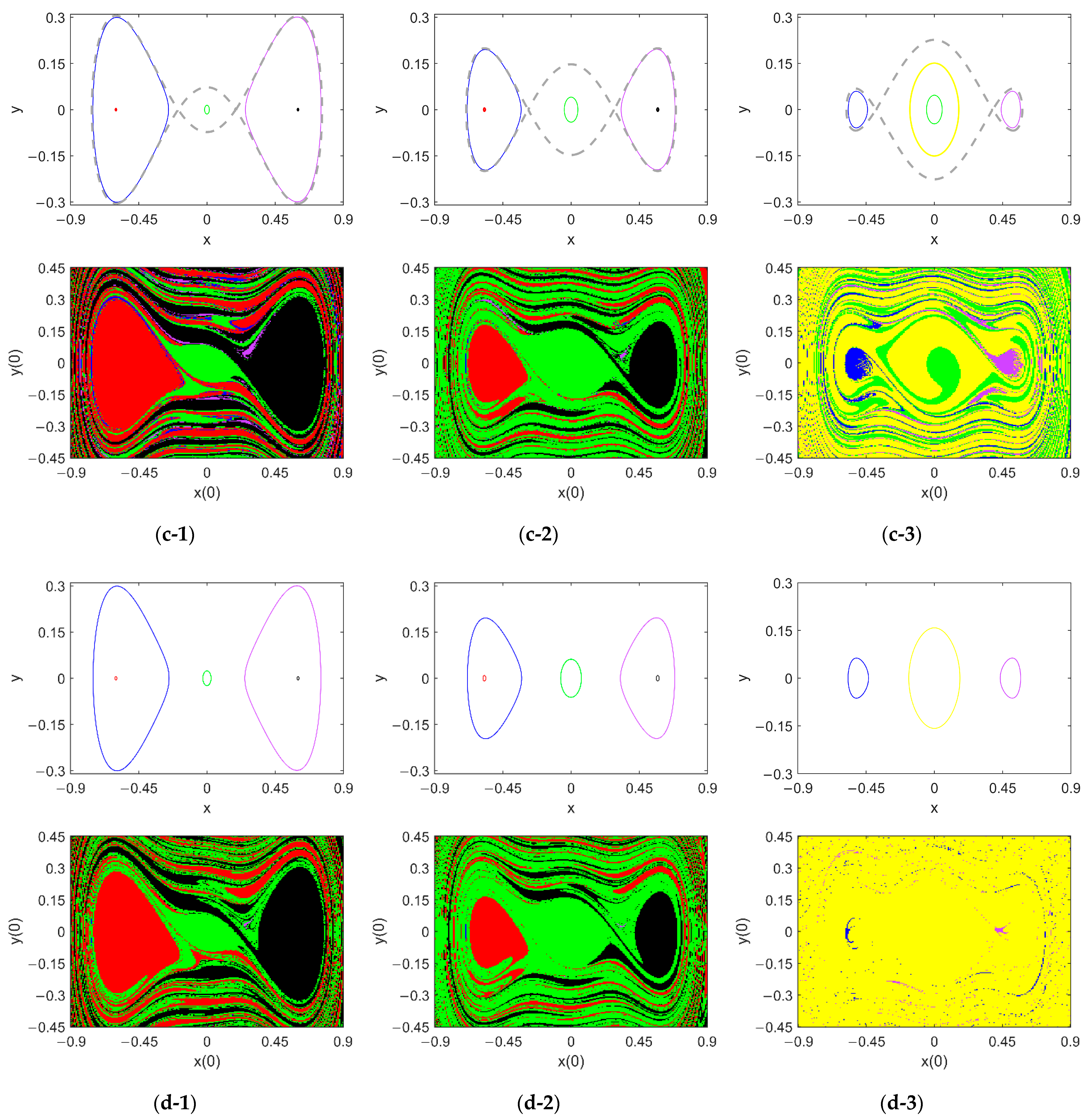
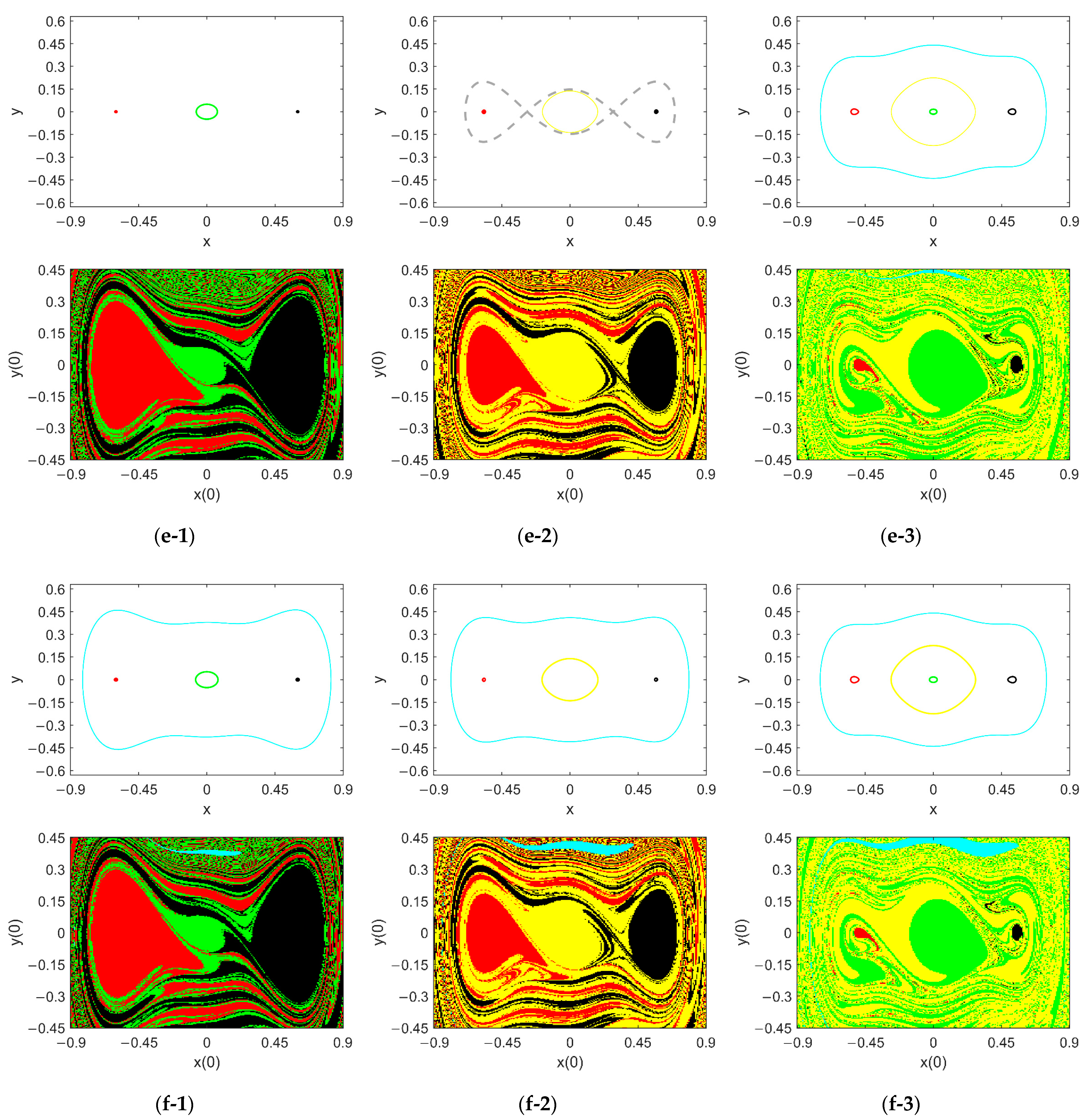
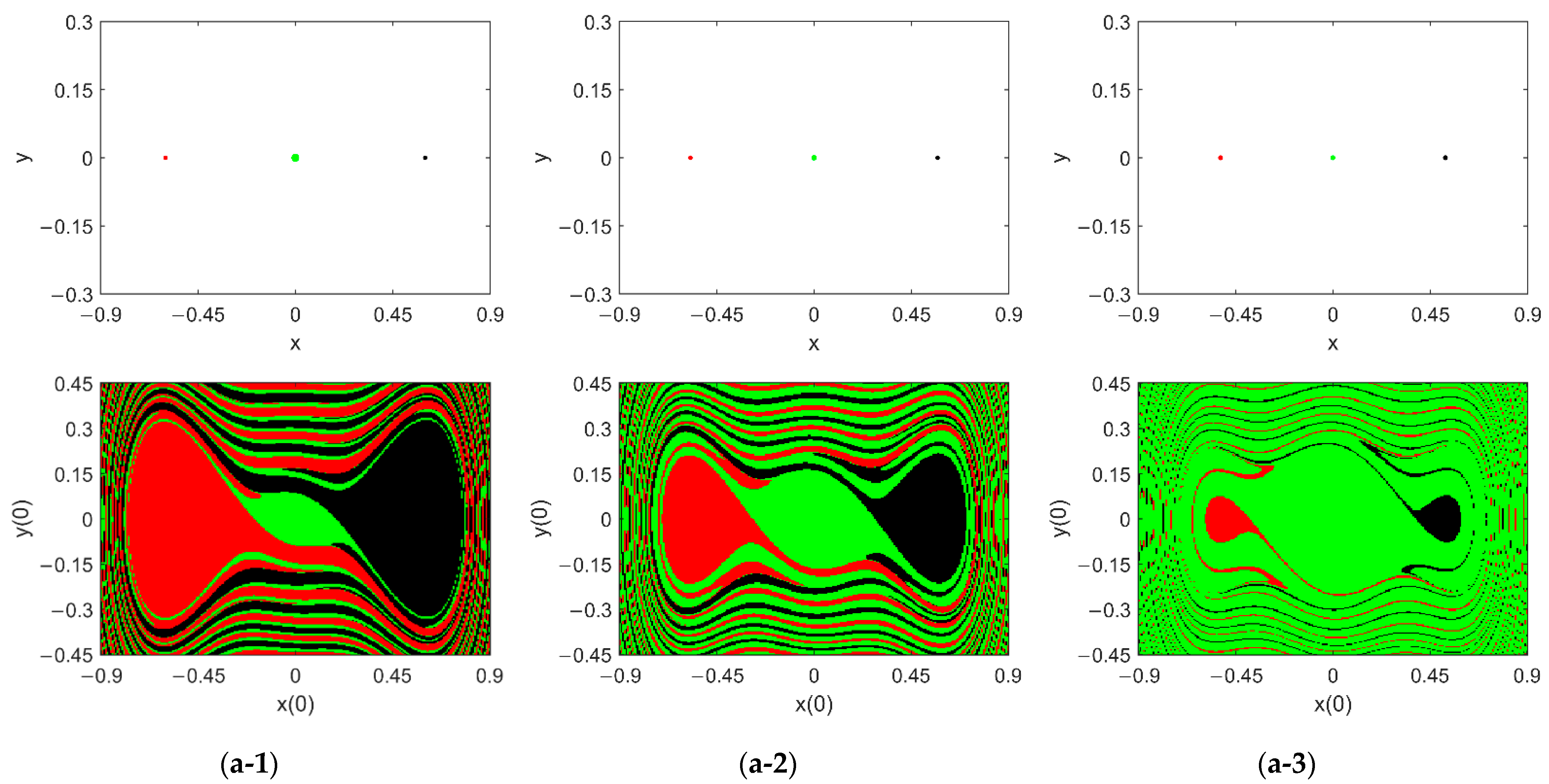
4.1. Coexisting Responses and Their BAs at ω = 0.9

For ω = 0.9, the evolution of the coexisting attractors and their BAs with the increase in the excitation level at c ^ = 0.36 , c ^ = 0.37 , and c ^ = 0.38 is shown in the first, second, and third columns of Figure 9, respectively.
As f0 varies from 0.001 to 0.003, there is only a monostable response around each of the three centers when c ^ = 0.36 and c ^ = 0.37 (see Figure 9(a-1)–(b-3)). Since the boundaries of their corresponding BAs in the vicinity of each potential well center are smooth, the tristable responses are locally dynamically integrated and reliable. Considering their amplitudes are very low, the PEH system at c ^ = 0.36 and c ^ = 0.37 only harvests very little vibration energy. In contrast, at c ^ = 0.38 , there are bistable responses around each nontrivial center C ± ( ± x c , 0 ) , as it can be seen in Figure 9(c-1,c-2). The occurrence of bistability around each nontrivial center was predicted in the previous section, which is validated by the numerical results in this section. And with the increase in f0, the erosion of the BA of the lower amplitude response by the BA of the higher amplitude one becomes more visible. Since a higher amplitude response corresponds to a higher voltage output, it can be concluded that, for ω = 0.9 and a very weak ambient excitation, the performance of the PEH system for energy harvesting is much better at c ^ = 0.38 than at c ^ = 0.36 and c ^ = 0.37 .
When f0 increases to 0.007, bistability around each nontrivial center also appears in system (4) at c ^ = 0.36 and c ^ = 0.37 (see Figure 9(c-1,c-2)). Even though the new attractors are of much higher amplitudes, their BAs are so small and fractal that they are called rare and hidden attractors [32,33,34]. Accordingly, it is almost impossible for system (3) to achieve these attractors. In other words, these higher amplitude attractors at c ^ = 0.36 and c ^ = 0.37 can hardly contribute to the energy collection process. Meanwhile, as shown in the blue loops, the purple ones, and the dashed ones in Figure 9(c-1)–(c-3), the trajectories of the higher amplitude attractors in the vicinity of C ± ( ± x c , 0 ) nearly touch the homoclinic orbits, which means the occurrence of homoclinic bifurcation. The fractal boundaries of the BAs of the higher amplitude attractors around C ± ( ± x c , 0 ) can be ascribed to homoclinic bifurcation, which usually leads to the erosion of BAs [35]. For c ^ = 0.38 , the lower amplitude attractors around C ± ( ± x c , 0 ) vanish (see Figure 9(c-3)). Even though the BAs of the bigger attractors are a little fractal in the vicinity of C ± ( ± x c , 0 ) , considering that they dominate most of the initial state area around C ± ( ± x c , 0 ) , and the BA eroding them belongs to the largest attractor, the performance of the PEH system at c ^ = 0.38 is enhanced with the increase in f0. Still, at f0 = 0.007, the system performs the best at c ^ = 0.38 .
When f0 = 0.012, the BAs of all the attractors around C ± ( ± x c , 0 ) are apparently shrunken in size. Still, at c ^ = 0.36 and c ^ = 0.37 , the BAs of smaller attractors occupy the vicinity of the nontrivial well centers, and the BAs of the higher amplitude attractors are still barely visible in the initial plane, as it can be observed in Figure 9(d-1,d-2). The system can harvest more energy when its initial condition is in the vicinity of the trivial equilibrium as the amplitude of the corresponding attractor is higher than that of the smaller attractors around C ± ( ± x c , 0 ) . At c ^ = 0.38 (see Figure 9(d-3)), the attractors around C ± ( ± x c , 0 ) become rare attractors, and the BA of the largest attractor is dominated in the initial state plane, as shown in the yellow region. Hence, the energy-harvesting performance continues to improve at c ^ = 0.38 .
When f0 exceeds 0.0125, the inter-well response appears at c ^ = 0.38 , which provides the possibility of the highest power output (see the light blue trajectory and BA in Figure 9(e-3)). This verifies our analysis about the minimum potential energy difference in Table 2. According to its BA, the inter-well attractor is a rare and hidden attractor. To show the attractor in full, we expanded the phase plane in Figure 9(e-1)–(e-3). At c ^ = 0.36 and c ^ = 0.37 , the higher amplitude periodic attractors around C ± ( ± x c , 0 ) become period-2 attractors, which are also hidden attractors. Considering that the amplitude of the attractor whose BA occupies most area of the initial plane at c ^ = 0.38 is much higher than the locally dynamically integrated ones at c ^ = 0.36 and c ^ = 0.37 (see the yellow, green, red, and black regions in Figure 9(e-1)–(e-3)), one can conclude that the performance of the PEH is still the best at c ^ = 0.38 .
Therefore, when ω = 0.9, among the three values of c ^ , the value of 0.38 implies an overwhelming advantage in energy harvesting.

4.2. Coexisting Responses and Their BAs at ω = 0.7

Given ω = 0.7, we present the evolution of the responses and their BAs with the increase in f0 at the three values of c ^ in Figure 10.
For f0 = 0.001, in the vicinity of each center, there is only one attractor with a very low amplitude (see Figure 10(a-1)–(a-3)), implying a very low power output at the three values of c ^ .
For f0 = 0.003, there is no change in the global dynamics of system (1) at c ^ = 0.36 (see Figure 10(b-1)), and only in the vicinity of O(0, 0), the power output can be higher, as the response displacement is the largest among the triple responses. At c ^ = 0.37 and c ^ = 0.38 , higher amplitude intra-well attractors appear in the neighborhood of O(0, 0) and C ± ( ± x c , 0 ) , respectively (see the yellow, blue, and purple curves and regions in Figure 10(b-2,b-3)). The former can contribute to increasing the voltage output as its BA erodes the vicinity of the trivial equilibrium, while the latter is useless in harvesting energy because the corresponding BAs are too dispersed to be detected (see Figure 10(b-3)). Hence, the system performs the best at c ^ = 0.37 when f0 = 0.003.
As it can be observed in Figure 10(b-3), where c ^ = 0.38 , the trajectories of the intra-well responses around C ± ( ± x c , 0 ) come very close to the homoclinic orbits, which indicates the homoclinic bifurcation and the erosion of BAs of the responses around C ± ( ± x c , 0 ) . From then on, with the increase in the excitation level, the shrinking of the corresponding BAs becomes more and more noticeable (see the red and black BAs in Figure 10(c-3,d-3,e-3,f-3)). This illustrates that, at c ^ = 0.38 , the effect of intra-well responses around C ± ( ± x c , 0 ) on energy harvesting becomes lower with the increase in f0.
As f0 is increased to 0.005, the global dynamics does not change at c ^ = 0.36 and c ^ = 0.37 (see Figure 10(c-1,c-2)). In this case, the attractor around O(0, 0) at c ^ = 0.36 is enlarged, and the BA of the higher amplitude attractor around O(0, 0) at c ^ = 0.37 is further expanded in the vicinity of O(0, 0), which are both beneficial for energy harvesting. Differently, at c ^ = 0.38 , a new attractor with a much higher amplitude appears whose BA is not near O(0, 0); thus, it is still a hidden attractor contributing little to energy collection.
As f0 increases to 0.01, the amplitudes of the attractors around the centers are enlarged, which can be observed in Figure 10(d-1)–(d-3). At c ^ = 0.37 and c ^ = 0.38 , the BAs of the larger attractors surrounding O(0, 0) are also enlarged (see the yellow regions in Figure 10(d-2,d-3)), illustrating that, with the increase in f0, the performance of the PEH system in energy harvesting is improved. Specifically, at c ^ = 0.37 , the BA of the larger intra-well attractor occupies most areas of the vicinity of the trivial equilibrium, demonstrating that, in the vicinity of O(0, 0), the system at c ^ = 0.37 can harvest more energy than at c ^ = 0.36 or c ^ = 0.38 . Meanwhile, at c ^ = 0.38 , the higher amplitude responses in the vicinity of C ± ( ± x c , 0 ) vanish, and BAs of the intra-well attractors around C ± ( ± x c , 0 ) are further eroded by the BAs of the two attractors around O(0, 0) (see the fractal green and yellow regions in Figure 10(d-3)). In this case, since the amplitudes of the green, black, and red attractors are nearly the same and much lower than that of the yellow attractor, a tiny disturbance to the initial conditions in the vicinity of C ± ( ± x c , 0 ) may lead to the better energy-harvesting performance. In contrast, at c ^ = 0.36 or c ^ = 0.37 , the BAs of the small attractors around C ± ( ± x c , 0 ) are still very large. It follows from Figure 10(d-1)–(d-3) that, in the vicinity of the trivial equilibrium, the system has the best performance in energy harvesting at c ^ = 0.37 , while in the vicinity of the nontrivial equilibria, the system performs the best at c ^ = 0.38 .
For f0 = 0.011, the situation is the same at c ^ = 0.36 (see Figure 10(e-1)). At c ^ = 0.37 , the smaller intra-well attractor around O(0, 0) vanishes, and the BA of the larger one occupies the potential well around O(0, 0), thus further enhancing the energy-harvesting efficiency. It means an escape from the potential wells surrounded by the heteroclinic orbits, namely, the heteroclinic bifurcation. As it usually leads to the basin erosion of the intra-well attractors [36], the occurrence of fractal fingers on the boundary of the yellow region in Figure 10(e-2) can be ascribed to the heteroclinic bifurcation. At c ^ = 0.38 , a large-displacement inter-well attractor can be observed. Since its BA is small and outside of the potential wells, it is a hidden attractor that hardly contributes to energy collection. To depict it completely, we expanded the phase plane. The higher amplitude response trajectory comes very close to the heteroclinic orbits, as can also be observed in the yellow loop and the grey dashed curve in Figure 10(e-2).
For f0 = 0.012, at c ^ = 0.36 and c ^ = 0.37 , large-displacement inter-well responses also occur, but as in the case at c ^ = 0.38 , they contribute very little for the promotion of the energy conversion efficiency (see the light blue loops and regions in Figure 10(f-1)–(f-3)). At c ^ = 0.38 , the larger attractor is enlarged, and its BA in the vicinity of O(0, 0) expands, showing the promotion of the possibility in achieving this attractor. As its amplitude is much higher than the locally reliable attractors at c ^ = 0.36 or c ^ = 0.37 , the PEH performance at c ^ = 0.38 becomes the best.
When f0 is increased to 0.02, the BA of the inter-well attractor at each value of c ^ further expands, yet remains significantly distant from the equilibrium points. As a result, it is almost useless for the performance improvement of the PEH. At c ^ = 0.36 , one can also observe the fractal basin of the attractor around O(0, 0). According to the comparison between the green phase map and the grey heteroclinic orbits in Figure 10(g-1), it can be due to a heteroclinic bifurcation. At c ^ = 0.37 , new period-2 attractors appear whose BAs occupy a considerable part of the vicinity of C ± ( ± x c , 0 ) , thus leading to the possibility of harvesting more vibration energy (see Figure 10(g-2)); meanwhile, the BA of the higher amplitude attractor around O(0, 0) is seriously eroded, which is surely disadvantageous for energy harvesting. At c ^ = 0.38 , the attractors around C ± ( ± x c , 0 ) disappear; instead, the BAs of the attractors around the origin occupy the neighborhood of C ± ( ± x c , 0 ) , which can result in a larger displacement final response and a higher power output. In the vicinity of O(0, 0), the BA of the larger intra-well attractor continues to expand. Hence, when f0 = 0.02, the energy harvesting performance of the PEH is the best at c ^ = 0.38 .
To sum up, in the case of ω = 0.7 , the PEH oscillatory system can perform the best in energy harvesting at c ^ = 0.37 if the excitation level is low, while it may achieve the best performance at c ^ = 0.38 when the excitation level is high enough to induce an inter-well response.

4.3. Coexisting Responses and Their BAs at ω = 0.5

Given ω = 0.5, the sequences of the coexisting attractors and their BAs with the increase in the excitation level at the three different values of c ^ are shown in Figure 11.
For f0 = 0.001, the amplitudes of the tristable intra-well attractors are very low and their BAs are separated by clearly delineated basin boundaries. Among the three values of c ^ , 0.36 is the best value for c ^ in this case, as the amplitude of the attractor around O(0, 0) is the highest when c ^ = 0.36 , as shown in Figure 11(a-1).
For f0 = 0.003, one can observe bistability around the trivial equilibrium at c ^ = 0.36 (see Figure 11(b-1)). The BA of the higher amplitude response occupies a part of the vicinity of O(0, 0), thus providing a high possibility of the boost of voltage output. At c ^ = 0.37 and c ^ = 0.38 , the global dynamics remains unchanged. Consequently, the PEH system still works the best at c ^ = 0.36 .
The situation remains the same for f0 = 0.005 or f0 = 0.006. At c ^ = 0.38 , the global dynamics of system (4) remains unchanged with the increase in f0; thus, the system can harvest very little energy. At c ^ = 0.37 , bistability appears in the vicinity of the initial state (0, 0). However, the higher amplitude attractor is almost unhelpful in increasing the power output of the PEH as it is a rare and hidden attractor. At c ^ = 0.36 , the BA of the lower amplitude attractor around O(0, 0) is severely eroded by the BA of the larger one at f0 = 0.005; even at f0 = 0.006, the lower amplitude attractor disappears, and the vicinity of the initial state (0, 0) is occupied by the BA of the higher amplitude response (see Figure 11(c-2)), meaning that the performance of the PEH system is improved with the increase in f0.
When f0 is increased to 0.007, 0.36 is not necessarily the best choice for c ^ because the BA of the largest intra-well response is seriously fractal in the vicinity of the origin. It means a high possibility of a sudden reduction in power output as a small disturbance to the initial state from (0, 0) may induce a jump from the largest attractor to a much smaller one. Comparatively, the largest attractor at ĉ = 0.37 has a continuous BA in the vicinity of the origin (see the green loop and region in Figure 11(e-2)), while the two attractors around the nontrivial equilibria at ĉ = 0.38 also have continuous BAs (see the red and black loops and regions in Figure 11(e-3)). Accordingly, for f0 = 0.007, the performance of the PEH system depends on the initial conditions: if the initial state is in the vicinity of the nontrivial equilibria, the system performs best at c ^ = 0.38 ; if the initial state is in the vicinity of the trivial equilibrium, the reliability and locally dynamic integrity is the best at c ^ = 0.37 .
As f0 continues to increase, this situation remains unchanged. For example, at f0 = 0.0105, the largest attractor at c ^ = 0.36 becomes a rare and hidden one, as displayed in Figure 11(f-1). And in Figure 11(f-3)–(g-2), the new inter-well responses and period-2 ones at the three different values of c ^ are also hidden attractors; thus, the collection of energy cannot rely on them. It is worth mentioning that, for f0 = 0.02, the BA of the large-displacement inter-well response is very close to the nontrivial centers C ± ( ± x c , 0 ) (see Figure 11(g-3)), implying a high possibility of boosting the energy-harvesting efficiency by the disturbance to the initial state in the vicinity of the right nontrivial center.
It can be concluded from Figure 11 that, at ω = 0.5, the PEH system performs the best at c ^ = 0.36 when the excitation level is too low to induce the erosion of BA in the vicinity of O(0, 0); when the excitation level is high enough to trigger the inter-well responses at the three different values of c ^ , the PEH system performs the best if c ^ = 0.37 and the initial state is near O(0, 0) or if c ^ = 0.38 and the initial state is in the vicinity of the nontrivial equilibria.
It follows from the comparison of Figure 9, Figure 10 and Figure 11 that the reduction in the excitation frequency makes the energy harvesting of the PEH system more difficult. Regarding the value of the structural parameter c ^ , if the ambient excitation level is low, for ω = 0.5, ω = 0.7, or ω = 0.9, the system performs the best in collecting energy at c ^ = 0.36 , c ^ = 0.37 , or c ^ = 0.38 , respectively. The reason is that the excitation frequency is within the frequency band for bistability around O(0, 0) at each value of c ^ . Differently, if the excitation level is high enough to induce inter-well responses, the PEH system performs the best in the vicinity of the nontrivial equilibria at c ^ = 0.38 . Since the parameter c ^ is decided by the value of the vertical distance between the two pins on the base, it implies that the maximum distance among the three vertical distances can be more advantageous to harvest vibration energy at a high ambient excitation level.

5. Discussion

In this study, multistability mechanisms for enhancing the energy-harvesting performance of a piezoelectric energy harvester (PEH) with geometrical nonlinearities were discussed in detail. The coupling effects of the ambient excitation, structural parameters, and the disturbance to the initial state on the final response of the PEH oscillatory system were taken into consideration.
To begin with, the geometrically nonlinear PEH oscillatory system and its nondimensional system were derived. In order to configure the triple potential wells of the oscillatory system, static bifurcation diagrams in the structural parameter plane were depicted. On this basis, the vertical distance between the two pins on the base of the PEH was considered as the key structural parameter of which three reasonable values were chosen for comparing and evaluating the performances of the PEH under them.
Next, using the method of multiple scales, the intra-well resonant responses were investigated. Since the coexistence of bistable resonant responses may broaden the useful frequency bandwidth for energy harvesting, we calculated the frequency bands for bistability within each potential well at different values of the key parameter. It was found that the intra-well bistability can be yielded by the stiffness softening characteristics of the system due to the saddle-node bifurcation of the periodic solutions. At each value of the key distance, the resonant frequency in the vicinity of the trivial equilibrium as much lower than the one in the vicinity of the nontrivial centers. Hence, between the frequency bands for bistability around the trivial and nontrivial well centers, the former was more practical and useful as the ambient excitation frequency is usually much lower than the resonant frequency of the device. And the resonant responses perturbed from the trivial center can achieve more power output; thus, attention should be paid to them. It followed from the theoretical prediction and the numerical results that, with the decrease in the vertical distance between the two pins on the base of the PEH, the frequency band for bistability around the origin became lower, which was beneficial for harvesting energy effectively in a low-frequency environment.
Then, to validate the qualitative results and further study the effect of the key parameter on the dynamics of the PEH oscillatory system, numerical simulations using the fourth-order Runge–Kutta approach and the cell mapping method were conducted to depict the sequences of the coexisting attractors and their basins of attraction with the increase in the excitation level. Without the loss of fairness, three values of the frequency were chosen successively from the bands of intra-well bistability around the origin at the three values of the key parameter to represent the low frequencies of the ambient excitation.
The quantitative results illustrate that, between the bistable responses near each nontrivial center, the higher amplitude resonant response is a hidden and rare attractor that can hardly be achieved, thus contributing almost nothing to energy harvesting. In contrast, in the vicinity of the trivial center, the higher amplitude resonant response coexisting with the lower amplitude one can increase the power output of the PEH system as it can be easily achieved as the final response. With the increase in the excitation level, the amplitude of an intra-well attractor grows so large that the escape of the trajectories from the potential well surrounded by the homo/heteroclinic orbits, namely, the homo/heteroclinic bifurcation, can be induced, thus successively leading to the erosion of BAs of the attractors within the well, the period-n responses, and the inter-well responses. Since the basin erosion of an attractor means the loss of the dynamic integrity and reliability of the attractor, the erosion of the BAs in the vicinity of the trivial equilibria is disadvantageous for energy harvesting. For the inter-well responses that coexist with the intra-well ones, even though their displacements are significantly larger, they may contribute little to the energy harvesting of the PEH system. This is because the initial conditions to trigger them are usually so distant from the three centers that it is hard to achieve them in practical applications.
Comparing the performances of the PEH system at the different values of the vertical distance between the two pins on the base, it was found that, when the level of the environmental excitation is very low, deciding which one among the three values of the key structural parameter is the best for improving the performance of the PEH system depends on the range of the excitation frequency; when the excitation level increases sufficiently to induce inter-well responses, the maximum one is the best for improving the performance of the PEH. The findings suggest that, by leveraging multistability effects, it is possible to optimize the operation range and increase the overall power output in piezoelectric energy harvesters.
This study highlighted the potential benefits offered by incorporating multistability mechanisms into the design of geometrically nonlinear PEHs. Due to simplicity of the primary structure and the convenience of adjusting the key structural parameter of the PEH, a practical device based upon the theoretical model will be manufactured in the future. Experiments will be conducted to assess the energy-harvesting performance and the reliability of the PEH in our next work. Efforts will be made to explore additional aspects, such as scalability, cost-effectiveness, and long-term stability, before implementing these concepts on a larger scale.

Author Contributions

Conceptualization, H.S.; methodology, H.S.; software, Z.W.; validation, H.S.; formal analysis, H.S.; investigation, Z.W.; writing—original draft preparation, Z.W. and H.S.; writing—review and editing, H.S.; visualization, Z.W.; supervision, H.S.; project administration, H.S.; funding acquisition, H.S. All authors have read and agreed to the published version of the manuscript.

Funding

This research was funded by the National Natural Science Foundation of China, grant number 11472176.

Institutional Review Board Statement

Not applicable.

Informed Consent Statement

Not applicable.

Data Availability Statement

Data are contained within the article.

Acknowledgments

Huilin Shang acknowledges the support of the National Natural Science Foundation of China under grant number 11472176. The authors are grateful for the valuable comments of the reviewers.

Conflicts of Interest

The authors declare no conflicts of interest.

References

  1. Amin Karami, M.; Inman, D.J. Powering pacemakers from heartbeat vibrations using linear and nonlinear energy harvesters. Appl. Phys. Lett. 2012, 100, 042901. [Google Scholar] [CrossRef]
  2. Yang, X.; LI, Z.; Wang, S.; Dou, Y.; Zhan, Y.; Zhao, R. Applicability of bridge vibration energy harvester based on nonlinear energy sink. J. Vib. Shock 2022, 41, 64–70. [Google Scholar]
  3. Bendine, K.; Hamdaoui, M.; Boukhoulda, B.F. Piezoelectric energy harvesting from a bridge subjected to time-dependent moving loads using finite elements. Arab. J. Sci. Eng. 2019, 44, 5743–5763. [Google Scholar] [CrossRef]
  4. Sezer, N.; Koç, M. A comprehensive review on the state-of-the-art of piezoelectric energy harvesting. Nano Energy 2021, 80, 105567. [Google Scholar] [CrossRef]
  5. Daqaq, M.F.; Masana, R.; Erturk, A.; Dane Quinn, D. On the Role of Nonlinearities in Vibratory Energy Harvesting: A Critical Review and Discussion. Appl. Mech. Rev. 2014, 66, 040801. [Google Scholar] [CrossRef]
  6. Ferrari, M.; Ferrari, V.; Guizzetti, M.; Marioli, D.; Taroni, A. Piezoelectric multifrequency energy converter for power harvesting in autonomous microsystems. Sens. Actuators A Phys. 2008, 142, 329–335. [Google Scholar] [CrossRef]
  7. Li, H.; Qin, W.; Lan, C.; Deng, W.; Zhou, Z. Dynamics and coherence resonance of tri-stable energy harvesting system. Smart. Mater. Struct. 2016, 25, 1530038. [Google Scholar]
  8. Zhou, Z.; Qin, W.; Yang, Y.; Zhu, P. Improving efficiency of energy harvesting by a novel penta-stable configuration. Sens. Actuators A Phys. 2017, 265, 297–305. [Google Scholar] [CrossRef]
  9. Zhou, Z.; Qin, W.; Zhu, P. Improve efficiency of harvesting random energy by snap-through in a quad-stable harvester. Sens. Actuators A Phys. 2016, 243, 151–158. [Google Scholar] [CrossRef]
  10. Zhou, S.; Cao, J.; Lin, J. Theoretical analysis and experimental verification for improving energy harvesting performance of nonlinear monostable energy harvesters. Nonlinear Dyn. 2016, 86, 1599–1611. [Google Scholar] [CrossRef]
  11. Vocca, H.; Neri, I.; Travasso, F.; Gammaitoni, L. Kinetic energy harvesting with bistable oscillators. Appl. Energy 2012, 97, 771–776. [Google Scholar] [CrossRef]
  12. Litak, G.; Margielewicz, J.; Gąska, D.; Wolszczak, P.; Zhou, S. Multiple Solutions of the Tristable Energy Harvester. Energies 2021, 14, 1284. [Google Scholar] [CrossRef]
  13. Wang, C.; Zhang, Q.; Wang, W.; Feng, J. A low-frequency, wideband quad-stable energy harvester using combined nonlinearity and frequency up-conversion by cantilever-surface contact. Mech. Syst. Signal Process. 2018, 112, 305–318. [Google Scholar] [CrossRef]
  14. Fan, K.; Tan, Q.; Liu, H.; Zhang, Y.; Cai, M. Improved energy harvesting from low-frequency small vibrations through a monostable piezoelectric energy harvester. Mech. Syst. Signal Process. 2019, 117, 594–608. [Google Scholar] [CrossRef]
  15. Zhao, S.; Erturk, A. On the stochastic excitation of monostable and bistable electroelastic power generators: Relative advantages and tradeoffs in a physical system. Appl. Phys. Lett. 2013, 102, 103902. [Google Scholar] [CrossRef]
  16. Wang, G.; Liao, W.; Yang, B.; Wang, X.; Xu, W.; Li, X. Dynamic and energetic characteristics of a bistable piezoelectric vibration energy harvester with an elastic magnifier. Mech. Syst. Signal Process. 2018, 105, 427–446. [Google Scholar] [CrossRef]
  17. Kim, P.; Seok, J. Dynamic and energetic characteristics of a tri-stable magnetopiezoelastic energy harvester. Mech. Mach. Theory 2015, 94, 41–63. [Google Scholar] [CrossRef]
  18. Zheng, Y.; Wang, G.; Zhu, Q.; Li, G.; Zhou, Y.; Hou, L.; Jiang, Y. Bifurcations and nonlinear dynamics of asymmetric tri-stable piezoelectric vibration energy harvesters. Commun. Nonlinear Sci. 2023, 119, 107077. [Google Scholar] [CrossRef]
  19. Wang, G.; Zheng, Y.; Zhu, Q.; Liu, Z.; Zhou, S. Asymmetric tristable energy harvester with a compressible and rotatable magnet-spring oscillating system for energy harvesting enhancement. J. Sound Vib. 2023, 543, 117384. [Google Scholar] [CrossRef]
  20. Panyam, M.; Daqaq, M.F. Characterizing the effective bandwidth of tri-stable energy harvesters. J. Sound Vib. 2017, 386, 336–358. [Google Scholar] [CrossRef]
  21. Cao, Q.; Wiercigroch, M.; Pavlovskaia, E.E.; Grebogi, C.; Thompson, J.M. Archetypal oscillator for smooth and discontinuous dynamics. Phys. Rev. E Stat. Nonlin. Soft Matter Phys. 2006, 74, 046218. [Google Scholar] [CrossRef] [PubMed]
  22. Wang, Z.; Shang, H. Multistability and Jump in the Harmonically Excited SD Oscillator. Fractal Fract. 2023, 7, 314. [Google Scholar] [CrossRef]
  23. Ramlan, R.; Brennan, M.J.; Mace, B.R.; Kovacic, I. Potential benefits of a non-linear stiffness in an energy harvesting device. Nonlinear Dyn. 2009, 59, 545–558. [Google Scholar] [CrossRef]
  24. Jiang, W.; Chen, L. Snap-through piezoelectric energy harvesting. J. Sound Vib. 2014, 333, 4314–4325. [Google Scholar] [CrossRef]
  25. Foupouapouognigni, O.; Buckjohn, C.N.D.; Siewe, M.S.; Tchawoua, C. Hybrid electromagnetic and piezoelectric energy harvester with Gaussian white noise excitation. Phys. A Stat. Mech. Its Appl. 2018, 509, 346–360. [Google Scholar] [CrossRef]
  26. Younesian, D.; Alam, M.-R. Multi-stable mechanisms for high-efficiency and broadband ocean wave energy harvesting. Appl. Energy 2017, 197, 292–302. [Google Scholar] [CrossRef]
  27. Yang, T.; Cao, Q. Dynamics and performance evaluation of a novel tristable hybrid energy harvester for ultra-low level vibration resources. Int. J. Mech. Sci. 2019, 156, 123–136. [Google Scholar] [CrossRef]
  28. Yang, T.; Cao, Q. Dynamics and high-efficiency of a novel multi-stable energy harvesting system. Chaos Soliton. Fract. 2020, 131, 109516. [Google Scholar] [CrossRef]
  29. Cao, J.; Zhou, S.; Wang, W.; Lin, J. Influence of potential well depth on nonlinear tristable energy harvesting. Appl. Phys. Lett. 2015, 106, 173905. [Google Scholar] [CrossRef]
  30. Kim, P.; Son, D.; Seok, J. Triple-well potential with a uniform depth: Advantageous aspects in designing a multi-stable energy harvester. Appl. Phys. Lett. 2016, 108, 243902. [Google Scholar] [CrossRef]
  31. Han, Y.; Cao, Q.; Chen, Y.; Wiercigroch, M. A novel smooth and discontinuous oscillator with strong irrational nonlinearities. Sci. China Phys. Mech. 2012, 55, 1832–1843. [Google Scholar] [CrossRef]
  32. Dong, C.; Wang, J. Hidden and coexisting attractors in a novel 4d hyperchaotic system with no equilibrium point. Fractal Fract. 2022, 6, 306. [Google Scholar] [CrossRef]
  33. Guo, Z.; Wen, J.; Mou, J. Dynamic Analysis and DSP Implementation of Memristor Chaotic Systems with Multiple Forms of Hidden Attractors. Mathematics 2022, 11, 24. [Google Scholar] [CrossRef]
  34. Zhu, Y.; Shang, H. Global Dynamics of the Vibrating System of a Tristable Piezoelectric Energy Harvester. Mathematics 2022, 10, 2894. [Google Scholar] [CrossRef]
  35. Shang, H. Pull-in instability of a typical electrostatic MEMS resonator and its control by delayed feedback. Nonlinear Dyn. 2017, 90, 171–183. [Google Scholar] [CrossRef]
  36. Shang, H.; Xu, J. Delayed feedbacks to control the fractal erosion of safe basins in a parametrically excited system. Chaos Soliton. Fract. 2009, 41, 1880–1896. [Google Scholar] [CrossRef]
Figure 1. Simplified diagram of the geometrically nonlinear PEH.
Fractalfract 08 00041 g001
Figure 2. Static bifurcation diagrams for different values of r: (a) r = 1; (b) r = 5; (c) r = 9.
Fractalfract 08 00041 g002
Figure 3. Unperturbed orbits for different values of c ^ : (a) c ^ = 0.36; (b) c ^ = 0.37; (c) c ^ = 0.38.
Fractalfract 08 00041 g003
Figure 4. Variation in the potential energy function V(x) with the displacement x.
Fractalfract 08 00041 g004
Figure 5. Variation in the amplitudes of the intra-well periodic responses with the dimensionless excitation frequency at different dimensionless excitation levels: (a) f0 = 0.003; (b) f0 = 0.005.
Fractalfract 08 00041 g005
Figure 6. (a) The amplitudes of the periodic solutions vs. f0 at different excitation frequencies: (a) ω = 0.5; (b) ω = 0.7; (c) ω = 0.9.
Fractalfract 08 00041 g006
Figure 7. Amplitudes of the periodic solutions around the nontrivial equilibria versus the excitation frequency ω at low excitation levels: (a) f0 = 0.001; (b) f0 = 0.003.
Fractalfract 08 00041 g007
Figure 8. Amplitudes of the periodic solutions around C ± versus f0 at different excitation frequencies: (a) ω = 0.5; (b) ω = 0.7; (c) ω = 0.9.
Fractalfract 08 00041 g008
Figure 9. Evolution of the coexisting attractors and their BAs with the increase in f0 when ω = 0.9. (a-1) Attractors and their BAs at c ^ = 0.36 and f0 = 0.001. (a-2) Attractors and their BAs at c ^ = 0.37 and f0 = 0.001. (a-3) Attractors and their BAs at c ^ = 0.38 and f0 = 0.001. (b-1) Attractors and their BAs at c ^ = 0.36 and f0 = 0.003. (b-2) Attractors and their BAs at c ^ = 0.37 and f0 = 0.003. (b-3) Attractors and their BAs at c ^ = 0.38 and f0 = 0.003. (c-1) Attractors and their BAs at c ^ = 0.36 and f0 = 0.007. (c-2) Attractors and their BAs at c ^ = 0.37 and f0 = 0.007. (c-3) Attractors and their BAs at c ^ = 0.38 and f0 = 0.007. (d-1) Attractors and their BAs at c ^ = 0.36 and f0 = 0.012. (d-2) Attractors and their BAs at c ^ = 0.37 and f0 = 0.012. (d-3) Attractors and their BAs at c ^ = 0.38 and f0 = 0.012. (e-1) Attractors and their BAs at c ^ = 0.36 and f0 = 0.0125. (e-2) Attractors and their BAs at c ^ = 0.37 and f0 = 0.0125. (e-3) Attractors and their BAs at c ^ = 0.38 and f0 = 0.0125.
Fractalfract 08 00041 g009aFractalfract 08 00041 g009bFractalfract 08 00041 g009c
Figure 10. Evolution of the attractors and their BA with the increase in f0 when ω = 0.7. (a-1) Attractors and their BAs at c ^ = 0.36 and f0 = 0.001. (a-2) Attractors and their BAs at c ^ = 0.37 and f0 = 0.001. (a-3) Attractors and their BAs at c ^ = 0.38 and f0 = 0.001. (b-1) Attractors and their BAs at c ^ = 0.36 and f0 = 0.003. (b-2) Attractors and their BAs at c ^ = 0.37 and f0 = 0.003. (b-3) Attractors and their BAs at c ^ = 0.38 and f0 = 0.003. (c-1) Attractors and their BAs at c ^ = 0.36 and f0 = 0.005. (c-2) Attractors and their BAs at c ^ = 0.37 and f0 = 0.005. (c-3) Attractors and their BAs at c ^ = 0.38 and f0 = 0.005. (d-1) Attractors and their BAs at c ^ = 0.36 and f0 = 0.01. (d-2) Attractors and their BAs at c ^ = 0.37 and f0 = 0.01. (d-3) Attractors and their BAs at c ^ = 0.38 and f0 = 0.01. (e-1) Attractors and their BAs at c ^ = 0.36 and f0 = 0.011. (e-2) Attractors and their BAs at c ^ = 0.37 and f0 = 0.011. (e-3) Attractors and their BAs at c ^ = 0.38 and f0 = 0.011. (f-1) Attractors and their BAs at c ^ = 0.36 and f0 = 0.012. (f-2) Attractors and their BAs at c ^ = 0.37 and f0 = 0.012. (f-3) Attractors and their BAs at c ^ = 0.38 and f0 = 0.012. (g-1) Attractors and their BAs at c ^ = 0.36 and f0 = 0.02. (g-2) Attractors and their BAs at c ^ = 0.37 and f0 = 0.02. (g-3) Attractors and their BAs at c ^ = 0.38 and f0 = 0.02.
Fractalfract 08 00041 g010aFractalfract 08 00041 g010bFractalfract 08 00041 g010cFractalfract 08 00041 g010d
Figure 11. Evolution of the attractors and their BAs with the increase in f0 when ω = 0.5. (a-1) Attractors and their BAs at c ^ = 0.36 and f0 = 0.001. (a-2) Attractors and their BAs at c ^ = 0.37 and f0 = 0.001. (a-3) Attractors and their BAs at c ^ = 0.38 and f0 = 0.001. (b-1) Attractors and their BAs at c ^ = 0.36 and f0 = 0.003. (b-2) Attractors and their BAs at c ^ = 0.37 and f0 = 0.003. (b-3) Attractors and their BAs at c ^ = 0.38 and f0 = 0.003. (c-1) Attractors and their BAs at c ^ = 0.36 and f0 = 0.005. (c-2) Attractors and their BAs at c ^ = 0.37 and f0 = 0.005. (c-3) Attractors and their BAs at c ^ = 0.38 and f0 = 0.005. (d-1) Attractors and their BAs at c ^ = 0.36 and f0 = 0.006. (d-2) Attractors and their BAs at c ^ = 0.37 and f0 = 0.006. (d-3) Attractors and their BAs at c ^ = 0.38 and f0 = 0.006. (e-1) Attractors and their BAs at c ^ = 0.36 and f0 = 0.007. (e-2) Attractors and their BAs at c ^ = 0.37 and f0 = 0.007. (e-3) Attractors and their BAs at c ^ = 0.38 and f0 = 0.007. (f-1) Attractors and their BAs at c ^ = 0.36 and f0 = 0.0105. (f-2) Attractors and their BAs at c ^ = 0.37 and f0 = 0.0105. (f-3) Attractors and their BAs at c ^ = 0.38 and f0 = 0.0105. (g-1) Attractors and their BAs at c ^ = 0.36 and f0 = 0.02. (g-2) Attractors and their BAs at c ^ = 0.37 and f0 = 0.02. (g-3) Attractors and their BAs at c ^ = 0.38 and f0 = 0.02.
Fractalfract 08 00041 g011aFractalfract 08 00041 g011bFractalfract 08 00041 g011cFractalfract 08 00041 g011d
Table 1. Parameters of system (1) and the physical meanings.
ParameterSymbol
Equivalent mass of the proof mass (kg) M
Equivalent damping of the mass (N.s/m) C
Stiffness coefficient of the vertical spring (N/m) K v
Stiffness coefficient for each inclined spring (N/m) K h
Relative displacement of the oscillator (cm) X
Displacement of the base (cm) Y
Vertical half distance between two pins (cm) c
Horizontal distance between the rotation shifts (cm) d
Time (s) t
Original length of each inclined spring (cm) L
Electro-mechanical coupling coefficient in relation to voltage (N/V) β 1
Electro-mechanical coupling coefficient in relation to current (A.s/m) β 2
Piezoelectric capacitance (F) C p
Equivalent resistive load ( k Ω ) R p
Voltage at time t (V) V ( t )
Excitation level (N)F
Excitation frequency (Hz) Ω
Table 2. Potential energy differences for different values of c ^ .
Potential Energy Difference c ^ = 0.36 c ^ = 0.37 c ^ = 0.38
Between the origin O ( 0 , 0 ) and the saddle point S + 0.00260.01080.0256
Between the center C + ( x c , 0 ) and the saddle point S + 0.04650.01990.0023
Table 3. Values of the resonant frequency ω ˜ at different values of c ^ .
Structural Parameter c ^ Resonant Frequency ω ˜
0.360.5574
0.370.7822
0.380.9522
Table 4. Resonant frequency ω ^ around C ± ( ± x c , 0 ) at different values of c ^ .
Structural Parameter c ^ Resonant Frequency ω ^
0.36 1.6353
0.37 1.4046
0.38 0.9516
Disclaimer/Publisher’s Note: The statements, opinions and data contained in all publications are solely those of the individual author(s) and contributor(s) and not of MDPI and/or the editor(s). MDPI and/or the editor(s) disclaim responsibility for any injury to people or property resulting from any ideas, methods, instructions or products referred to in the content.

