Article

Research on Application of Fractional Calculus Operator in Image Underlying Processing

1
School of Electronic Information and Artificial Intelligence, Leshan Normal University, Leshan 614000, China
2
Internet Natural Language Intelligent Processing Key Laboratory of Education Department of Sichuan Province, Leshan 614000, China
3
Key Laboratory of Detection and Application of Space Effect in Southwest Sichuan, Leshan 614000, China
4
Lab of IOT Application and Security, Leshan Normal University, Leshan 614000, China
*
Author to whom correspondence should be addressed.
Fractal Fract. 2024, 8(1), 37; https://doi.org/10.3390/fractalfract8010037
Submission received: 7 June 2023 / Revised: 13 October 2023 / Accepted: 2 November 2023 / Published: 5 January 2024

Abstract

:
Fractional calculus extends traditional, integer-based calculus to include non-integer orders, offering a powerful tool for a range of engineering applications, including image processing. This work delves into the utility of fractional calculus in two crucial aspects of image processing: image enhancement and denoising. We explore the foundational theories of fractional calculus together with its amplitude–frequency characteristics. Our focus is on the effectiveness of fractional differential operators in enhancing image features and reducing noise. Experimental results reveal that fractional calculus offers unique benefits for image enhancement and denoising. Specifically, fractional-order differential operators outperform their integer-order counterparts in accentuating details such as weak edges and strong textures in images. Moreover, fractional integral operators excel in denoising images, not only improving the signal-to-noise ratio but also better preserving essential features such as edges and textures when compared to traditional denoising techniques. Our empirical results affirm the effectiveness of the fractional-order calculus-based image-processing approach in yielding optimal results for low-level image processing.

1. Introduction

Fractional calculus, with its three-century history, was long confined to the realm of pure mathematical analysis and largely ignored by engineers [1,2,3,4,5]. It was not until Mandelbrot introduced fractal theory, linking Riemann–Liouville fractional calculus to Brownian motion in fractal media [6,7,8], that the field captured the attention of engineering technologists. Consequently, fractional calculus has evolved from an esoteric mathematical theory into a practical tool for modeling complex systems in various engineering disciplines. Recent research has demonstrated that fractional calculus operators exhibit memory and nonlocality—features that are particularly useful for describing materials with inherent memory and unique properties. Now, the theory is making inroads not only in foundational sciences but also in applied engineering fields, proving its practical utility [9]. Over the past decade, researchers have uncovered the broad applicability of fractional calculus in signal analysis and processing. Studies have introduced fractional calculus to traditional memristor elements and formulated various natural forms of fractional impedance [10,11,12]. Additionally, recent works have combined fractional calculus with classic swarm intelligence algorithms, spawning new methods such as fractional neural networks and fractional ant colony algorithms based on the fractional steepest descent approach; these algorithms have shown promising results [13,14,15,16,17]. In the realm of image processing, pioneering work by Pu et al. laid the groundwork for applying fractional calculus. They identified unique features such as “nonlocality” and “weak derivatives,” leading to its application in low-level digital image processing. Their research introduced six basic fractional differential operators and set the stage for a novel methodology based on fractional calculations [18,19].
Significant strides have also been made in image processing through fractional calculus. Hacini, for example, developed a bidirectional fractional-order derivative mask for edge detection and denoising in both real and synthetic images [20]. Zhang combined rough set theory with fractional-order differentiators to enhance image details through a 2D Fourier transform and adaptive fractional-order differential operators [21]. Li introduced an active contour method for noisy image segmentation, which employs adaptively defined fractional orders [22]. This method incorporates fractional differentiation with adaptively defined orders into the fitting term to manage noise during curve evolution. Moreover, Bai proposed a new variational model for image denoising and decomposition using fractional-order bounded variation space to emphasize cartoon-like patterns [23]. Researchers have successfully integrated fractional calculus with partial differential equations to devise innovative image-processing techniques [24,25,26]. Notable among them is Abirami’s variable-order fractional diffusion model for medical image denoising, based on the Caputo finite-difference scheme [27]. Building on Pu’s foundational work, numerous scholars have introduced novel image-processing models incorporating fractional calculus [28,29,30,31,32], such as methods based on fractional contrast-limited adaptive histogram equalization and denoising techniques using fractional-order NLM and BM3D.
This study investigates the application of fractional calculus theory to digital image processing. The remainder of the article is organized as follows: Section 2 delves into the mathematical and physical underpinnings of fractional calculus theory. Section 3 introduces the construction of fractional-order differential operators and assesses their effectiveness in image enhancement through simulations and comparative experiments. Section 4 is devoted to the development of fractional-order integral operators and evaluates their utility in image denoising via simulation experiments. Finally, Section 5 provides concluding remarks.

2. Basic Theory

This section offers a succinct overview of three central topics: (1) the core definitions of fractional calculus theory and their practical applications; (2) the amplitude–frequency characteristics of fractional-order differential and integral operators; and (3) the amplitude–frequency characteristics of typical signals when subjected to fractional calculus operations.

2.1. Fractional Calculus Theory

Although a unified time-domain expression for fractional calculus remains exclusive, several approaches have led to distinct definitions. Three classical definitions are particularly noteworthy: those of Grünwald–Letnikov, Riemann–Liouville, and Caputo, corresponding to Equations (1)–(3), respectively [1,2].
  • The Grünwald–Letnikov approach to fractional calculus is defined as follows:
    D a G t v f ( x ) = lim h 0   h v j = 0 t a h Γ ( v + j ) j ! Γ ( v ) f ( x j h )   v R
  • The Riemann–Liouville definitions for fractional-order integration and differentiation are as follows:
    D a R t v f ( x ) = 1 Γ ( v ) a t f ( y ) ( x y ) 1 v d y D a R t v f ( x ) = 1 Γ ( n v ) d n d t n a t f ( y ) ( x y ) 1 + v n d y
  • Caputo’s definition of fractional calculus is outlined as follows:
    D a C t v f ( x ) = D a R t v f ( x ) j = 0 m 1 f ( j ) ( a ) Γ ( j v + 1 ) ( t a ) k v
These three definitions of fractional calculus are closely related and can be transformed under certain conditions. The Riemann–Liouville and Caputo definitions serve as refinements of the original Grünwald–Letnikov definition. Specifically, the Grünwald–Letnikov approach is especially useful in signal processing applications because it can be converted into a convolution operation for numerical implementation. However, the Riemann–Liouville definition is mainly used to find analytical solutions for relatively straightforward functions. The Caputo definition proves particularly useful in engineering for analyzing initial boundary value problems in fractional-order differential equations.

2.2. Amplitude–Frequency Characteristics of Fractional Calculus Operators

2.2.1. Fractional-Order Differential Operator

Consider f ( x ) L 2 ( R ) as the square-integrable energy signal f ( x ) L 2 ( R ) , with its Fourier transform represented by f ( ω ) = R f ( x ) e i ω x d x . The n-th derivative of the signal f ( x ) is f n ( x ) ( n Z + ). Leveraging the properties of the Fourier transform, we can arrive at Equation (4).
D n f ( x ) F T ( D f ) n ( ω ) = ( i ω ) n f ( ω ) = d n ( ω ) f ( ω )
When we extend the positive integer n to a positive real number v ( v R + ), the fractional-order derivative of the signal f ( x ) can be expressed as f v ( x ) . Utilizing the properties of the fractional-order Fourier transform [33,34], we can formulate Equation (5), while d v ( ω ) can be further expanded to obtain Equation (6).
D v f ( x ) F T ( D f ) v ( ω ) = ( i ω ) v f ( ω ) = d v ( ω ) f ( ω )
d v ( ω ) = ( i ω ) v = α v ( w ) e i θ v ( ω ) α v ( w ) = ω v , θ v ( ω ) = v π 2 sgn ( ω )
According to Equations (5) and (6), the amplitude–frequency characteristic curve for the fractional-order differential operator of a one-dimensional signal can be plotted, as demonstrated in Figure 1a.
Based on Equations (5) and (6), Figure 1a delineates the amplitude–frequency characteristics of the fractional-order differential operator for one-dimensional signals. The curve reveals that the operator considerably boosts medium- and high-frequency signals. Specifically, this amplification rises nonlinearly and dramatically as both frequency and differential order increase.
In the extremely low-frequency range, the fractional-order differential operator modestly enhances the signal’s amplitude. Interestingly, this augmentation is marginally greater than what is achieved by first- and second-order differential operators.
In the medium-to-high-frequency range, the fractional-order differential operator amplifies the signal less than the first- and second-order operators do. This behavior highlights its “weak derivative” characteristics, allowing it not only to boost high-frequency components but also to nonlinearly maintain the very low-frequency elements.
From a signal processing viewpoint, this operator functions as a generalized form of amplitude and phase modulation. Its amplitude undergoes fractional-order exponential changes with frequency, while its phase aligns with a generalized Hilbert frequency shift.
As illustrated in Figure 1a and based on Equations (5) and (6), the amplitude–frequency characteristics of this fractional-order differential operator for one-dimensional signals reveal several key traits. First, the operator amplifies medium- and high-frequency signals, with this enhancement increasing nonlinearly and sharply as both frequency and differential orders rise. Second, at a specific fractional-order differential order v [ 0 , 1 ] , the operator amplifies the amplitude in the very low-frequency region ( ω < 1 ) to a certain extent, achieving an increase moderately greater than that of the first- and second-order operators. Lastly, in the mid-to-high-frequency region ( ω > 1 ) with v [ 0 , 1 ] , the operator does elevate the signal amplitude, but this increase is notably less than that offered by the first- and second-order operators.
Overall, these characteristics show that the fractional-order differential operator possesses “weak derivative” properties. It not only emphasizes the high-frequency components but also nonlinearly preserves the very low-frequency elements of the signal. Additionally, in signal processing terms, this operator acts as a generalized form of amplitude and phase modulation. The amplitude changes exponentially with frequency in a fractional way, and its phase corresponds to a generalized Hilbert frequency shift [18].

2.2.2. Fractional-Order Integral Operator

Let us consider a square-integrable energy signal represented by f ( t ) L 2 ( R ) , whose Fourier transform is f ( ω ) = R f ( t ) e i ω t d t . When v R , I = D 1 and v = v can be assumed to obtain the Fourier transform form of the fractional-order integral operator based on the G-L definition, they can be expressed as in Equation (7). This expression ( i ω ) v can be further expanded to yield Equation (8).
I v f ( t ) F T ( I f ) v ( ω ) = ( i ω ) v f ( ω ) = i v ( ω ) f ( ω )
i v ( ω ) = α v ( w ) e i θ v ( ω ) α v ( w ) = | ω | v , θ v ( ω ) = v π 2 sgn ( ω )
Based on Equations (7) and (8), Figure 1b illustrates the amplitude–frequency characteristics of the fractional-order integral operator for one-dimensional signals. Several observations emerge from a direct analysis. First, fractional-order integral operators attenuate medium- and high-frequency signals, an effect that intensifies nonlinearly as both frequency and the integration order rise. For a specific frequency range v [ 0 , 1 ] and order v [ 0 , 1 ] , the fractional-order integral operator modestly amplifies the signal amplitude. However, this amplification is significantly less than that achieved by first- and second-order integral operators. Within another v [ 0 , 1 ] frequency range and a particular order v [ 0 , 1 ] , the fractional-order integral operator lessens the signal amplitude, but this decrease is far less substantial than that generated by the first- and second-order integral operators. These attributes indicate that the fractional-order integral operator not only suppresses the high-frequency components of the signal but also maintains its highest-frequency components in a nonlinear way. Furthermore, while the amplitude of low-frequency elements is reduced, those at the very lowest frequencies are preserved.

2.3. Fractional-Order Calculus Processing and Analysis of Common Signals

Figure 2a–d display the amplitude–frequency characteristic curves for fractional calculus applied to various types of signals: a square wave (Equation (9)), a triangular wave (Equation (10)), a sinusoidal signal ( sin ( t ) ), and a Gaussian signal (Equation (11)). Analysis shows that as the order increases from 0 to 1 for the square wave, there is a significant enhancement in the fractional calculus output at points of abrupt change. Similarly, the results for the triangular wave evolve into a shape resembling a square wave. When the fractional derivative order is set at v = 1 , the curves represent the first derivatives of both the sinusoidal and Gaussian signals, indicating their maximum rate of change. For fractional-order differential values within v [ 0 , 1 ] , both the sinusoidal and Gaussian signals show a fractional-order continuous interpolation, linking the actual signal value with its most rapidly changing direction.
S q u a r e ( t ) = 1 0 t T 1 T < t 2 T
Triangular ( t ) = n = 1 4 E n π 2 sin 2 n π 2 cos n ω t
G a u s s ( t ) = 1 2 π e t 2 2
These findings highlight that the integer-order differential of a stationary point is zero, but its fractional-order differential is not. For signals that change linearly over time, the integer-order differential remains constant, while the fractional-order differential experiences nonlinear shifts. The unique characteristics of the fractional calculus operator enable it to emphasize details such as high-frequency edges and textures in images, while also preserving some low-frequency nuances to a degree. Therefore, image-processing techniques grounded in fractional calculus offer advantages over traditional methods based on integer orders. Specifically, this approach is more efficient in extracting intricate details such as edges and textures, while also maintaining the overall contour and texture information of the image.

3. Application of Fractional-Order Differential in Image Enhancement

In this section, we discuss two primary topics: (1) An examination of the characteristics of the fractional-order differential operator for image signals, which includes an image enhancement experiment rooted in fractional-order. This inquiry explores the relationship between the differential order of the fractional operator and the high-pass strength of a two-dimensional signal. (2) An image enhancement experiment using the fractional-order differential operator, which highlights the advantages of a fractional-order-based image enhancement algorithm over its integral-order counterpart.

3.1. Amplitude–Frequency Characteristics of Fractional-Order Differential Image Enhancement Operators

We can define the fractional-order v derivative of the two-dimensional energy function as f ( x , y ) be f v ( x , y ) ( v R + ). Owing to the separability of the fractional Fourier transform, it follows that the fractional-order differential filter for this two-dimensional energy function f v ( x , y ) is also separable. Therefore, based on Equation (5), we can derive the fractional-order differential filter function of the two-dimensional energy function f ( x , y ) , as presented in Equation (12).
( D f ) v ( ω x , ω y ) = | ω x | v e i v π 2 sgn ( ω x ) | ω y | v e i v π 2 sgn ( ω y )
The amplitude–frequency characteristic surface for two-dimensional signals, when applying differential operators of varying fractional orders, can be inferred from Equation (12) and is depicted in Figure 3. This figure delineates the amplitude–frequency characteristic surfaces of the fractional-order differential operator for orders v 0 , 0.1 , 0.5 , 1.0 . A close look at this figure reveals that the fractional-order differential operator serves as a high-pass filter. Notably, its cutoff frequency correlates with the fractional order of differentiation. As this order rises, the operator’s ability to filter high-frequency signals intensifies, effectively attenuating low-frequency elements in the image. The degree of this attenuation also escalates with the differential order.

3.2. Image Enhancement Experiment and Analysis of Fractional-Order Differential Operator

Under certain conditions, the fractional-order differentiation of two-dimensional image signals I ( x , y ) in both the X and Y directions can be considered separable [33,34]. Consequently, a normalized eight-direction fractional-order differentiation image enhancement operator can be obtained. The image signal’s duration [ a , t ] of the image signal I ( x , y ) is divided equally by step size h = 1 , expressed as, n = t a h = h = 1 t a , and the numerical formulations for the fractional-order differential operator along the X- and Y-axes can be found in Equations (13) and (14), where R x v ( x , y ) and R y v ( x , y ) represent the fractional-order differential remainders in the horizontal and vertical directions, respectively.
D a G t v I ( x , y ) x = Δ I ( x , y ) + ( v ) I ( x 1 , y ) + ( v ) ( v + 1 ) 2 I ( x 2 , y ) + ( v ) ( v + 1 ) ( v + 2 ) 6 I ( x 3 , y ) + R x v ( x , y )
D a G t v I ( x , y ) y = Δ I ( x , y ) + ( v ) I ( x , y 1 ) + ( v ) ( v + 1 ) 2 I ( x , y 2 ) + ( v ) ( v + 1 ) ( v + 2 ) 6 I ( x , y 3 ) + R y v ( x , y )
Figure 4 presents the fractional-order differential image-enhancement mask operator, denoted as W D . This operator is derived from Equations (13) and (14) to cover all eight directions in the image. While the fractional-order ladder degree is inherently a linear operator, its modulus becomes nonlinear due to the inclusion of square root calculations. As a result, the fractional-order ladder degree vector lacks rotationally invariant isotropy. However, as elaborated in Reference [35], the modulus of the fractional-order gradient vector is isotropic. This study’s fractional calculus operator demonstrated notable symmetry; specifically, the weights of the fractional calculus mask operator remain consistent across all eight directions in the digital image. The fractional-order gradient modulus value quantifies the outcomes in image processing. Thus, this fractional calculus operator possesses the feature of “anisotropic rotational variance.” The filtering coefficient for the fractional-order differential enhancement operator is provided in Equation (15).
W D 0 = 1 , W D 1 = v , W D 2 = v ( v + 1 ) 2 , W D 3 = v ( v + 1 ) ( v + 2 ) 6 , , W D m = v ( v + 1 ) ( v + 2 ) ( v + m 1 ) m !
To facilitate visual observation, Figure 5b–f display the inverted images processed by differential operators of varying orders ( v 0.1 , 0.5 , 0.8 , 1.0 , 2.0 ) on the Barbara images, to make visual observation more straightforward. Direct observation reveals that the image filtered by a fractional-order differential operator of order v = 0.1 enhances the image’s high-frequency details to some extent, while preserving a significant amount of low-frequency information. As the differential order increases, the fractional-order filtering operator progressively reduces the low-frequency content in the image, while nonlinearly amplifying the high-frequency details. When the image is filtered by a fractional-order differential operator with an order of v = 2.0, a substantial amount of low-frequency information is removed, leading to a nonlinear enhancement of the high-frequency elements in the image.
Figure 5 offers a visual comparison through a series of images. Figure 5b–f display Barbara images that have been processed using differential operators of varying orders v 0.1 , 0.5 , 0.8 , 1.0 , 2.0 . Direct observations show that a fractional-order differential operator with an order of v = 0.1 modestly amplifies the high-frequency details in the image while retaining a substantial amount of its low-frequency content. As the differential order increases, the fractional-order filtering operator progressively diminishes the low-frequency elements in the image and nonlinearly amplifies the high-frequency details. When the image undergoes processing with a differential order of v = 2.0, it loses a considerable amount of low-frequency content, while the high-frequency regions are significantly and nonlinearly enhanced.
Figure 6 displays the contrast variations in the Barbara image when processed by differential operators of different orders, specifically v 0.1 , 0.5 , 0.8 , 1.0 , 2.0 . Upon closer inspection, it is clear that when the image is enhanced using a fractional-order differential operator of order v = 0.1, the result is noticeably brighter, verging on overexposure. This outcome is due to the low-order differential filter’s capacity to preserve significant low-frequency contours and subtle textural nuances. Concurrently, the edge and texture details of the image receive moderate enhancement. In contrast, when the image is processed with a fractional-order differential operator of order v = 2.0, the resulting image does not show a dramatic increase in contrast. This can be attributed to the higher-order differential operator’s tendency to eliminate most of the low-frequency content while significantly accentuating the high-frequency edges and pronounced textural details, resulting in observable edge jitter.
Figure 7 presents a sequence of enhanced images. Specifically, Figure 7b,c feature images enhanced by fractional-order differential operators with orders v = 0.5 and v = 0.8, respectively. Figure 7d–f showcase images processed using classic integer-order differential enhancement operators: Sobel, Prewitt, and Laplacian. Figure 8 complements these by providing histograms corresponding to each image displayed in Figure 7.
Upon direct evaluation, fractional-order differential operators with v = 0.5 and v = 0.8 demonstrate significant capabilities. They effectively enhance subtle textural features in the smoother regions of the image, while nonlinearly amplifying stronger textural details, especially in areas with minor changes in gray value amplitude and frequency. Furthermore, these operators also significantly boost the high-frequency edge details, particularly in regions of the image characterized by substantial variations in gray value amplitude.
A side-by-side look at the histogram contrasts in Figure 8 yields an important insight: images processed using fractional-order differential enhancement operators tend to exhibit a more balanced gray level distribution. This leads to a superior overall image contrast compared to those processed with integer-order differential operators.
Table 1 provides a comparative analysis of experimental data from various image enhancement models. Direct analysis reveals that the fractional-order image enhancement model introduced in this study yields significant improvements in metrics such as average gradient, contrast, and image entropy. These improvements become particularly evident when contrasted with conventional integer-order image enhancement methods.

4. Application of Fractional-Order Integral in Image Denoising

This section delves into two key areas related to the application of fractional-order integration operators on image signals. (1) It explores the relationship between the integration order of fractional-order integral operators and the low-pass filtering strength in two-dimensional signals. (2) It underscores the advantages of fractional-order integral image-denoising operators over their integer-order counterparts. These advantages manifest both in subjective visual comparisons and objective performance metrics.

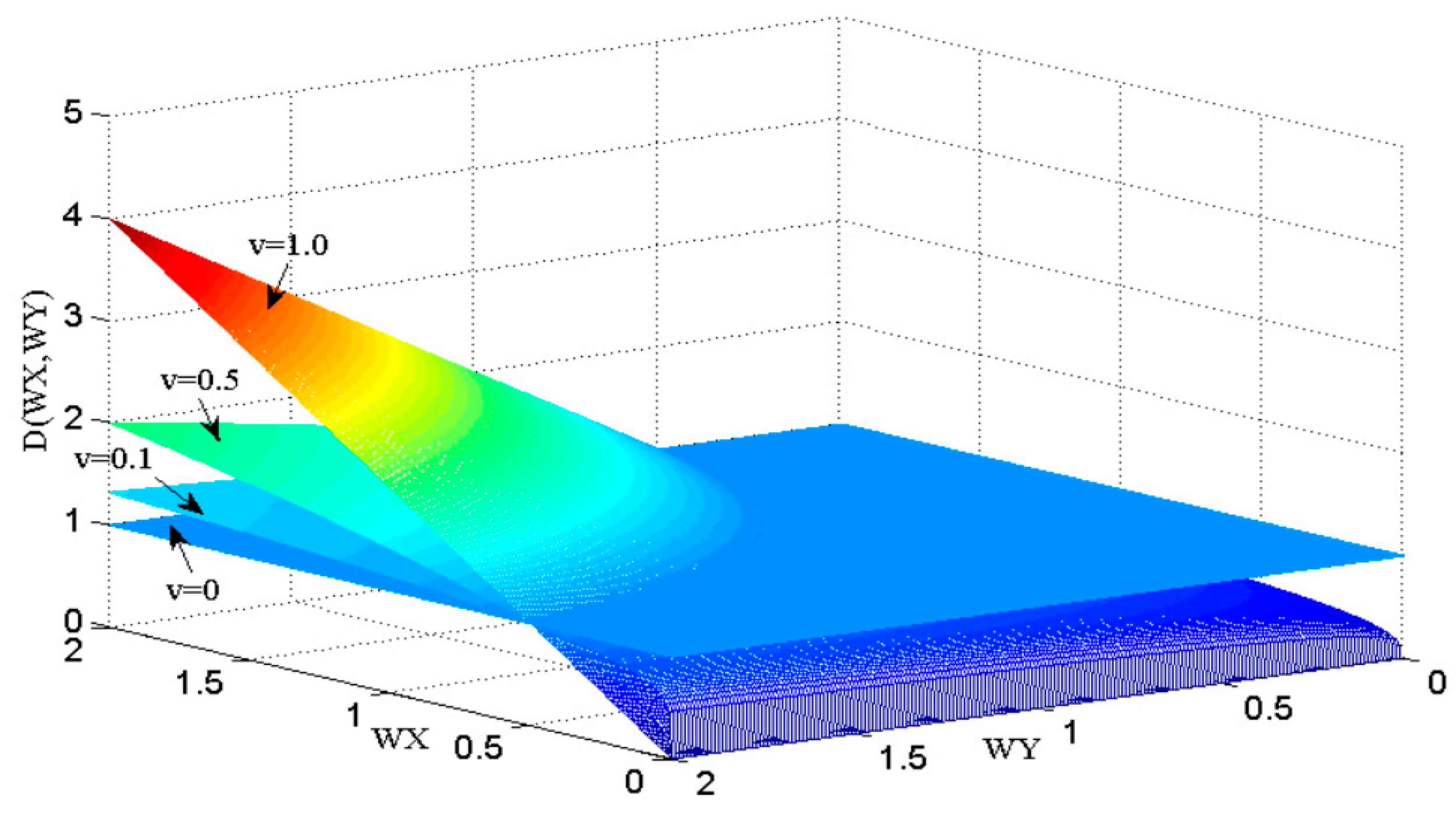
4.1. Amplitude–Frequency Characteristics of Fractional-Order Integral Operator Image Denoising Operator

Let the fractional-order integral of the two-dimensional energy function be denoted as f ( x , y ) be f v ( x , y ) ( v R ). Due to the separability of the fractional-order Fourier transform, the fractional-order integral filter of the two-dimensional energy function f ( x , y ) is also separable. Therefore, the fractional-order integral filter function of the two-dimensional energy function f ( x , y ) can be derived by expanding based on Equation (7), as illustrated in Equation (16).
( I f ) v ( ω x , ω y ) = | ω x | v e i v π 2 sgn ( ω x ) | ω y | v e i v π 2 sgn ( ω y )
Figure 9 displays the amplitude–frequency characteristic surfaces for fractional integration operators at different orders ( v 0.1 , 0.5 , 0.8 , 1.0 , 2.0 ), as derived from Equation (16). Direct observation confirms that these fractional-order integration operators act as low-pass filters. Moreover, their cutoff frequency is correlated with the fractional order of integration. As this order of integration increases, the low-pass performance of the operators is enhanced. Specifically, these fractional-order integration operators attenuate the high-frequency signals in images, and this attenuation effect grows nonlinearly as the integration order rises.
Figure 9 illustrates the amplitude–frequency characteristic surfaces for fractional integration operators at different orders v 0.1 , 0.5 , 0.8 , 1.0 , 2.0 as outlined in Equation (16). Direct evaluation indicates that these fractional-order integration operators serve as low-pass filters. Importantly, their cutoff frequency is directly related to the fractional integration order. As this order escalates, the effectiveness of low-pass filtering is amplified. In particular, these fractional-order integration operators diminish high-frequency components in the images, and this attenuation effect grows nonlinearly with an increase in the integration order.

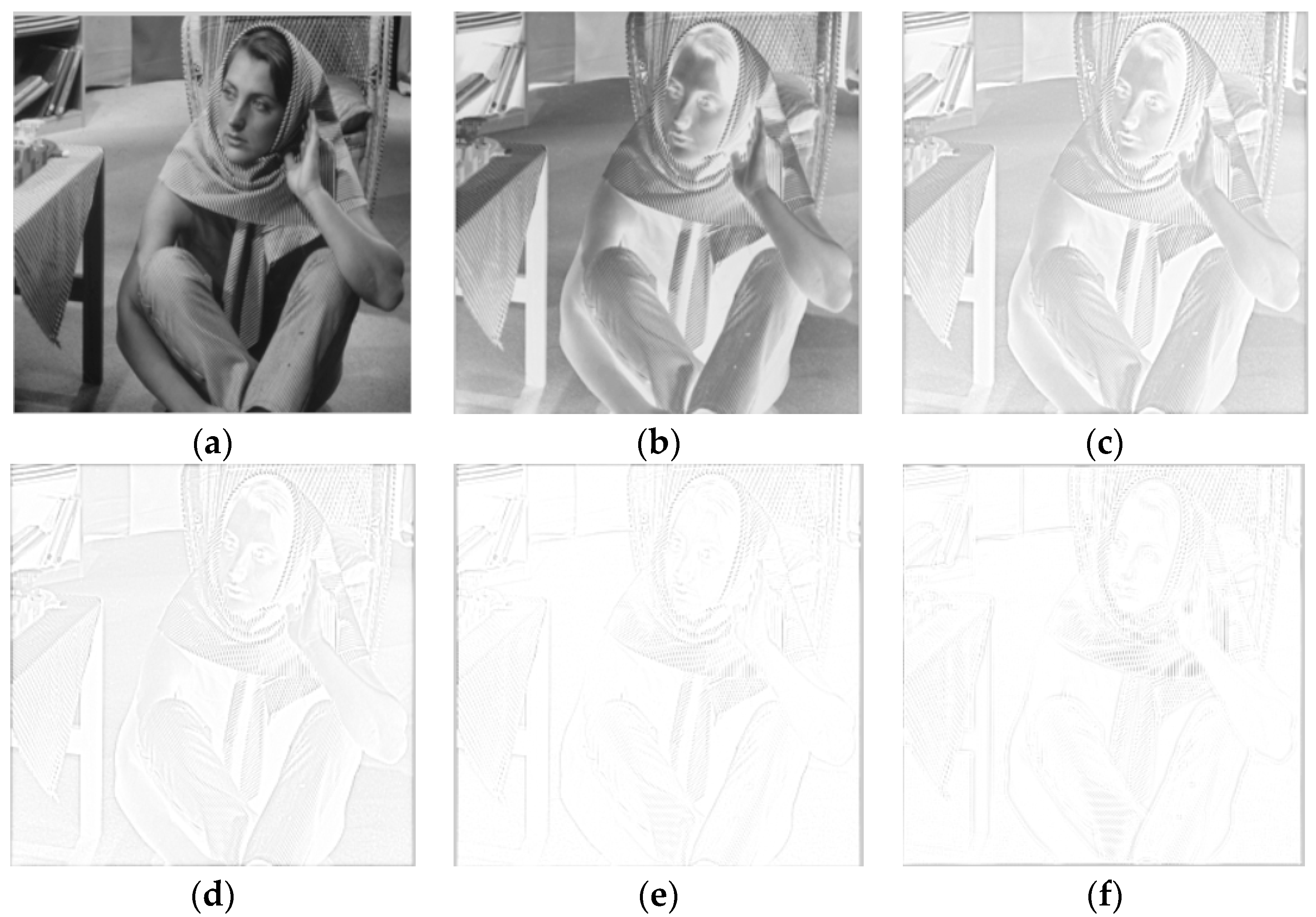
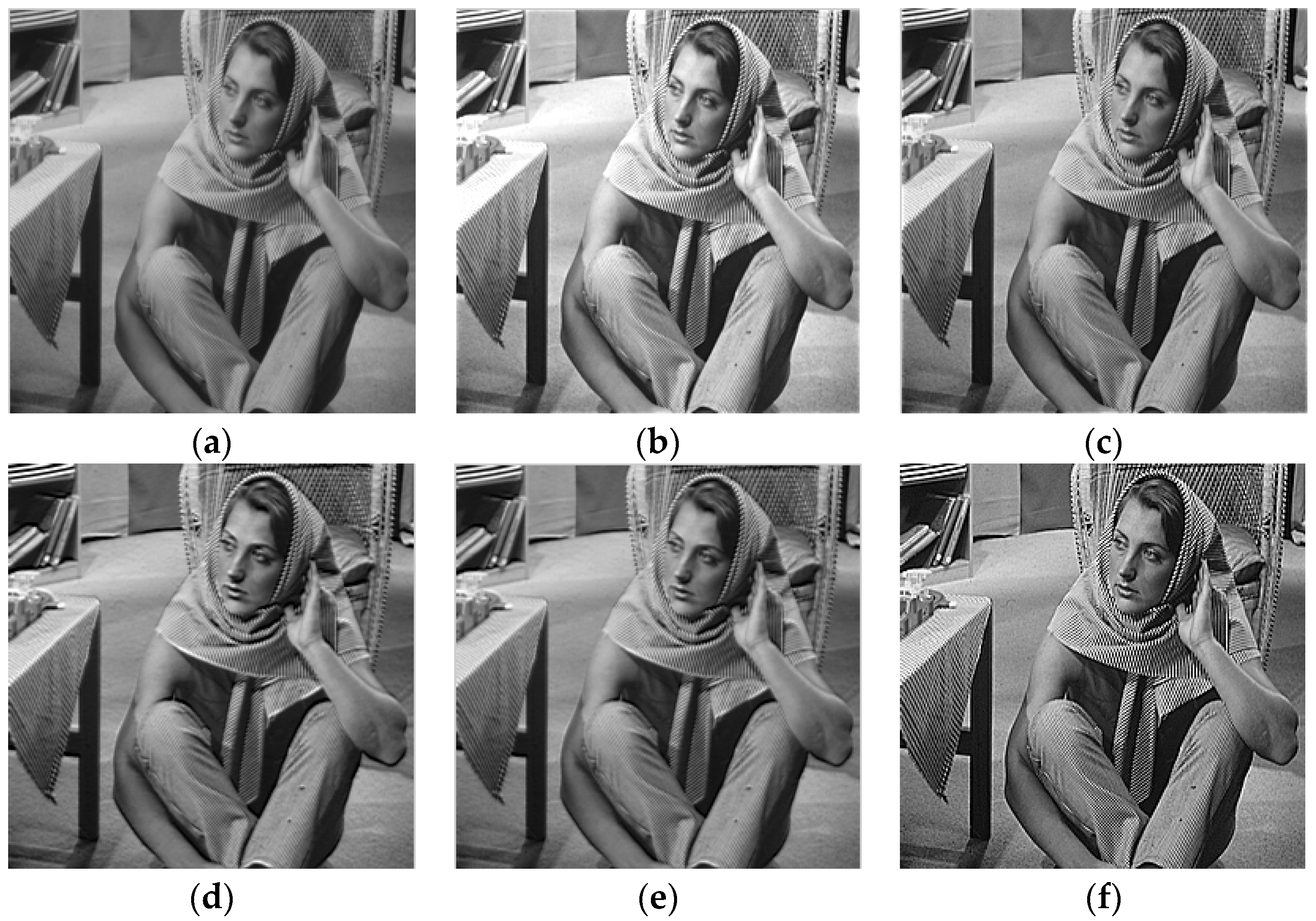
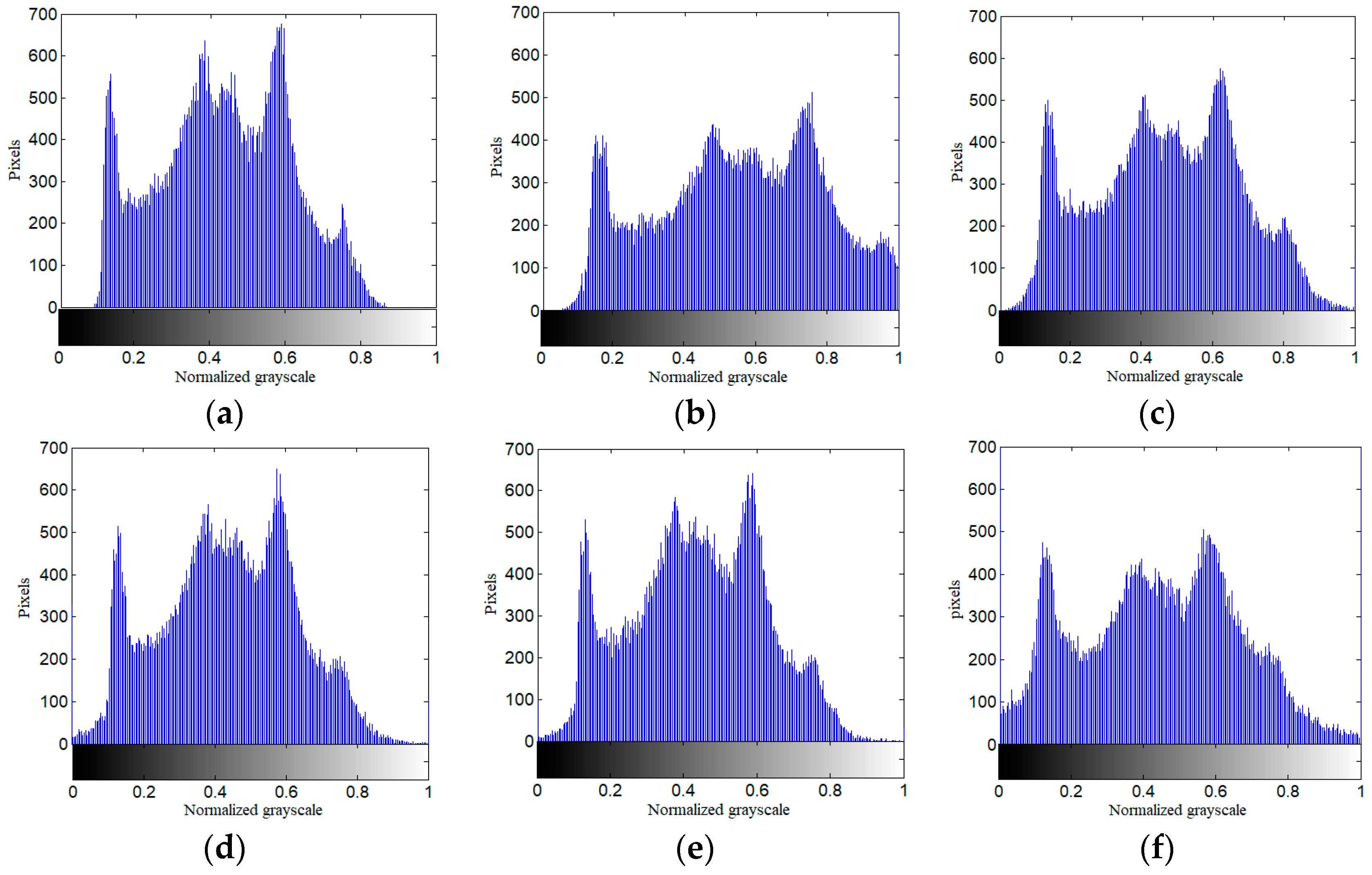
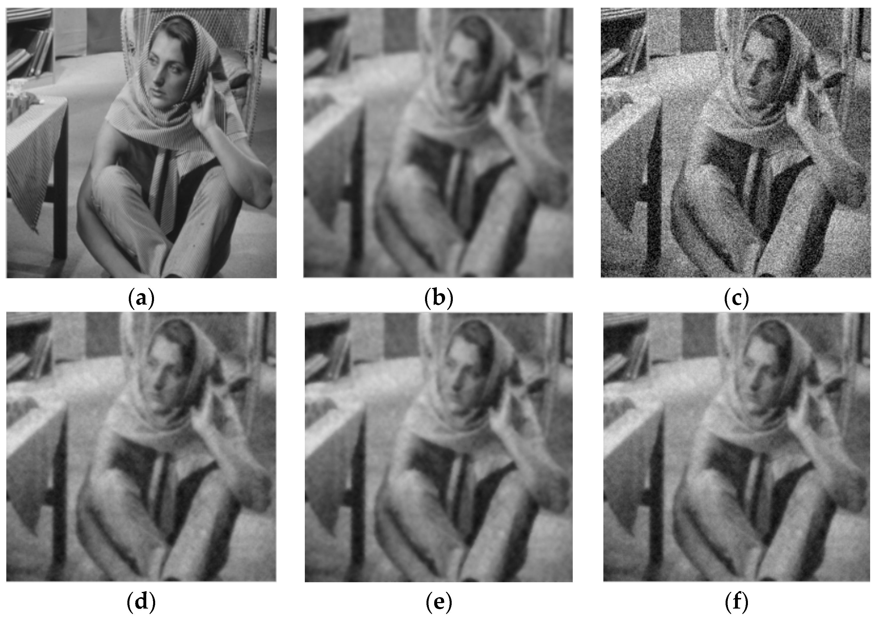
4.2. Experiment and Analysis of Fractional-Order Integral Operator for Image Denoising

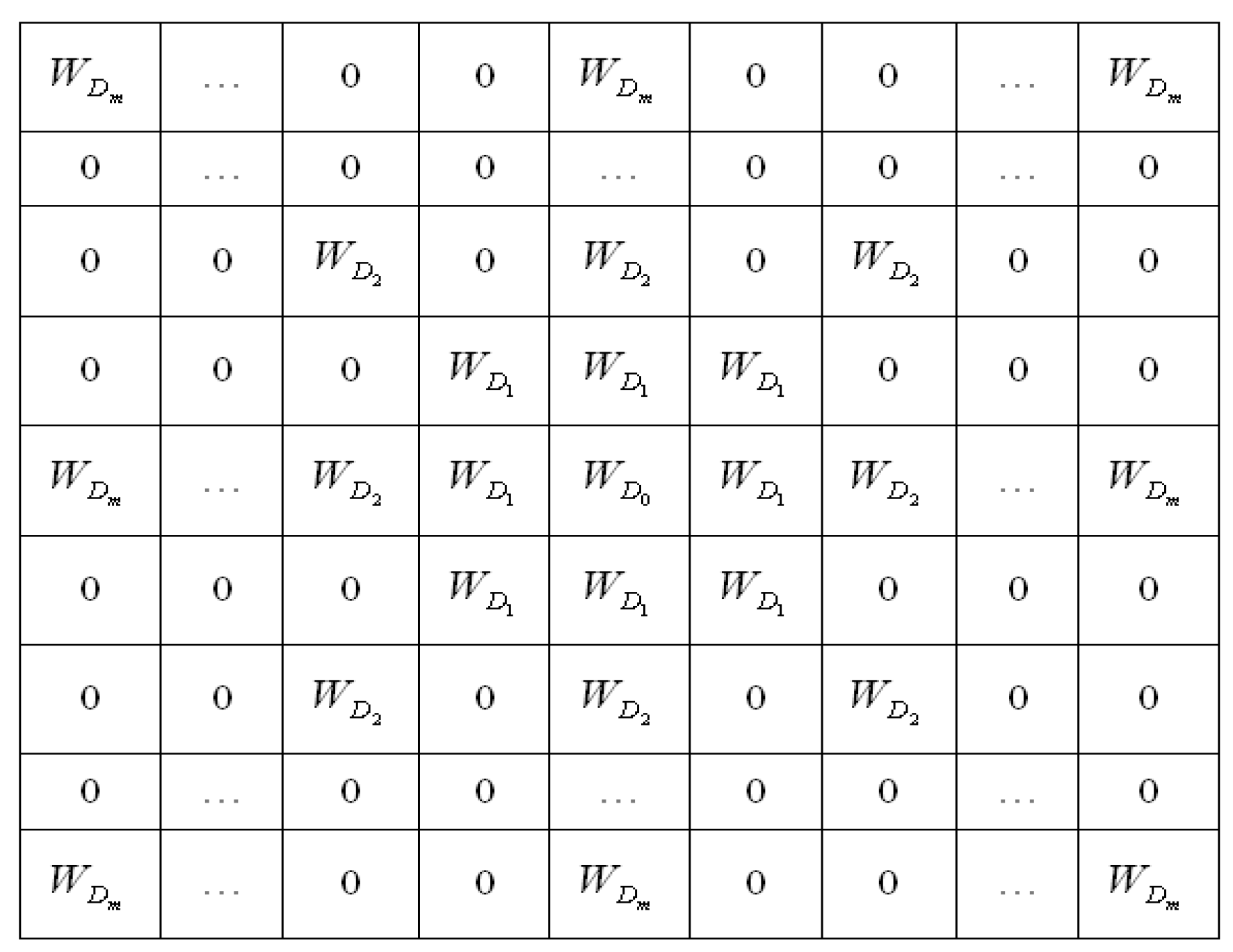
4.2.1. Construction of Fractional-Order Integral Operators

As previously stated, the fractional-order integration of two-dimensional image signals I ( x , y ) in both the X-axis and Y-axis directions is separable under specific conditions. For this study, we employed a normalized eight-direction fractional-order integration operator to denoise the images independently. The time span [ a , t ] of the image signal is I ( x , y ) partitioned into equal intervals, denoted as h = 1 .
As previously discussed, the fractional-order integration of two-dimensional image signals I ( x , y ) in the X- and Y-axes can be separated conditions. To denoise the images, we utilize a normalized eight-direction fractional-order integration operator on each axis independently. The duration of the image signal I ( x , y ) can be divided into equal intervals, i.e., n = t a h = h = 1 t a . The numerical expression for the fractional-order integration operator along the X- and Y-axes, as defined by the G-L method, is detailed in Equations (17) and (18). Here, R x v ( x , y ) and R x v ( x , y ) represent the residual terms of the fractional-order integration in the horizontal and vertical directions, respectively.
I a G t v I ( x , y ) x = Δ I ( x , y ) + v I ( x 1 , y ) + v ( v + 1 ) 2 I ( x 2 , y ) + v ( v + 1 ) ( v + 2 ) 6 I ( x 3 , y ) + R x v ( x , y )
I a G t v I ( x , y ) y = Δ I ( x , y ) + v I ( x , y 1 ) + v ( v + 1 ) 2 I ( x , y 2 ) + v ( v + 1 ) ( v + 2 ) 6 I ( x , y 3 ) + R y v ( x , y )
Figure 10 presents the fractional-order integral denoising operator W I , which expands upon Equations (19) and (20) to include the remaining six image directions, thereby creating an eight-direction denoising operator. The construction methodology for both fractional-order integral operators and fractional-order differential augmentation operators is analogous. According to Reference [35], fractional-order integral operators exhibit anisotropic rotation variance; the corresponding filtering coefficient is detailed in Equation (19).
Figure 10 displays the fractional-order integral denoising operator, W I , which extends Equations (19) and (20) to include six additional image directions, thereby yielding an eight-direction denoising operator. The construction of these fractional-order integral operators is similar to that of fractional-order differential augmentation operators. As highlighted in Reference [35], these integral operators also possess anisotropic rotation variance; the associated filtering coefficient is outlined in Equation (19).
W I 0 = 1 , W I 1 = v , W I 2 = v ( v + 1 ) 2 , W I 3 = v ( v + 1 ) ( v + 2 ) 6 , , W I m = v ( v + 1 ) ( v + 2 ) ( v + m 1 ) m !

4.2.2. Evaluation Criterion

  • Subjective Evaluation
    Subjective evaluation entails gauging enhanced image quality through direct human visual inspection, aiming to capture authentic human visual perceptions. This method proves particularly valuable as it involves firsthand interaction with the image using human vision [36,37]. Leveraging the human eye’s keen sensitivity to details such as texture and edges, we prioritize examining the edges and textural nuances to assess the overall visual impact of the denoised image.
  • Objective Evaluation
    • Objective evaluation, on the other hand, employs mathematical metrics tailored to mirror specific image qualities that align with human perception. The subsequent results are derived from certain image attributes based on the evaluation function. This study makes use of key metrics such as average gradient, edge preservation coefficient, and signal-to-noise ratio to critically compare the performance of different image-denoising operators [38].
    • Average Gradient (AG)
      The average gradient (AG) in an image serves as an indicator of contrast variations, reflecting the image’s textural and detail transitions. This offers insights into the image’s overall sharpness. The formula to calculate the AG value is provided in Equation (20).
      A G = 1 M N i = 1 r o w j = 1 c o l Δ horizontal f ( i , j ) 2 + Δ vertical f ( i , j ) 2
    • Edge Preservation Index (EPI)
      The edge preservation index gauges how effectively a filtering operator maintains the image’s horizontal or vertical edges. A higher EPI value signifies better edge preservation by the operator in question. The formula to compute this coefficient is outlined in Equation (21).
      E P I = i = 1 row j = 1 c o l Δ horizontal f a f t e r ( i , j ) + Δ vertical f a f t e r ( i , j ) i = 1 row j = 1 c o l Δ horizontal f b e f o r ( i , j ) + Δ vertical f b e f o r ( i , j )
    • Contrast (C)
      Image contrast refers to the relationship between the black and white intensities within an image, serving as a gradient scale that transitions from black to white. A higher contrast ratio suggests a broader spectrum of gradient levels, enhancing the image’s textural details. The methodology for determining the image’s contrast is encapsulated in Equation (22). Here, the parameter N u m b e r represents the logarithm of the differences in grayscale values among the image’s eight neighboring regions.
      C = i = 1 row j = 1 c o l Δ f ( i , j ) N u m b e r
    • Signal-to-Noise Ratio (SNR)
      Lastly, the signal-to-noise ratio (SNR) acts as a vital metric for assessing image quality. It quantifies the ratio between the magnitudes of the image signal and the noise, giving a numerical value to the image’s clarity. The expression for the SNR is elaborated upon in Equation (23).
      S N R = 10 × l g i = 1 r o w j = 1 c o l f ( i , j ) 2 i = 1 r o w j = 1 c o l | f ( i , j ) f d e n o i s e ( i , j ) | 2

4.2.3. Experimental Results and Comparative Analysis

Figure 11 displays the denoised Barbara image, processed using fractional-order integral image-denoising operators of varying orders and subjected to Gaussian white noise with a given mean μ = 0 and variance σ = 0.1 . Upon close inspection, it is evident that the operator with a fractional-order integration value of v = 0.1 exhibits limited denoising efficacy but retains most of the image’s edge and texture details. On the contrary, the operator with v = 1.0 shows strong denoising capabilities but significantly compromises the image’s edge and texture, resulting in a less visually pleasing outcome. The findings suggest that as the fractional order of the integration operator rises, its proficiency in noise reduction improves. However, this also leads to an increase in the attenuation of high-frequency information, causing more pronounced image blurring.
As illustrated in Figure 11, the Barbara image is denoised using fractional-order integral image-denoising operators of different orders, subjected to Gaussian white noise with a mean μ = 0 and variance σ = 0.1 . A close examination reveals that the operator with a fractional-order integration value of v = 0.1 has limited denoising capabilities but excellently preserves edge and texture details. In contrast, the operator with v = 1.0 performs admirably in noise reduction but sacrifices much of the image’s edge and texture, resulting in a visually disappointing outcome. These observations indicate that as the fractional order escalates, the operator becomes more effective in noise removal. However, this benefit is offset by an increase in the attenuation of high-frequency elements, causing the image to blur.
Figure 12 showcases the results of denoising the Barbara image, which is contaminated by Gaussian white noise with a particular mean μ = 0 and variance σ = 0.1 , using an array of denoising techniques. Specifically, Figure 12c features images processed through the mean method, Figure 12d through the Gaussian method, Figure 12e through the Wiener method, and Figure 12f using the fractional-order integration low-order iteration method. Complementing this, Figure 13 displays the inverted residual images that highlight the discrepancies between the processed and original images. Here, Figure 13a depicts the residual from the mean method, Figure 13b from the Gaussian method, Figure 13c from the Wiener method, and Figure 13d from the fractional-order integration low-order iteration method. Upon initial visual inspection, it becomes clear that the technique introduced in this study leverages a low-order fractional-order integral iterative denoising approach. Because of the choice of a smaller integration order, each denoising iteration tends to preserve the edge and texture details of the image more effectively than traditional integer-order strategies. This results in a subtler “micro-denoising” effect on noisy images. Table 2 offers a comprehensive comparison of key metrics, including AG values, edge preservation coefficients, and SNR values, following the application of various denoising methods. Visually, the low-order fractional-order integral iterative denoising technique put forth in this study seems to excel in retaining complex features like edges and textures, while also achieving an optimal SNR when compared with integer-order denoising strategies.
Table 2 provides a comparative analysis of experimental data from various image-denoising algorithms. When contrasted with traditional methods such as mean denoising, Gaussian denoising, and Wiener filtering, the fractional-order integration image-denoising approach shows marked improvements in key metrics (specifically, it enhances the AG, edge retention coefficient and signal-to-noise ratio) of the processed image to varying extents.

5. Conclusions

This work delves into image enhancement and denoising methods rooted in the principles of fractional calculus, bypassing the need to exploit an image’s self-similarity and local features. Initially, the paper outlines three canonical definitions of fractional calculus and explores the relevant applications of each. It then meticulously examines the amplitude–frequency characteristics of fractional calculus operators, highlighting the intricate relationship between high-pass and low-pass dynamics for both one-dimensional and two-dimensional signals in relation to the order of calculus. Building on these insights, we developed an image enhancement model using fractional-order differential operators and an image-denoising model grounded in fractional calculus operators.
Our empirical results affirm the effectiveness of the fractional-order calculus-based image processing approach presented in this paper. Specifically, we observed enhanced contrast and clarity when compared to traditional integer-order calculus methods, particularly in the realms of image amplification, coupled with its enhanced edge retention and denoising capabilities in image refinement. The endeavor to assimilate fractional-order calculus theory into foundational image processing teems with potential. Current scholarly discussions are geared toward developing innovative image-processing methods that integrate fractional-order calculus theory with established intelligent algorithms. One promising avenue for research is adaptive fractional-order image enhancement and denoising, where the operator adaptively determines the order magnitude of the fractional-order template based on local images features, as suggested by various scholars [39]. This approach is envisaged to yield optimal results in low-level image processing.
Looking forward, future studies may investigate the potential of leveraging fractional-order operators with distributed orders or nonsingular kernels to further improve results. As advancements in computer hardware continue, traditional intelligent algorithms are likely to evolve, paving the way for state-of-art fractional-order image-processing technologies to play a crucial role in practical applications.

Author Contributions

Conceptualization, G.H.; Methodology, G.H.; Software, G.H.; Validation, Q.C.; Formal analysis, G.H., Q.C. and Z.S.; Investigation, H.-y.Q. and Q.C.; Resources, S.J.; Data curation, S.J. and C.H.; Writing—original draft, G.H. and C.H.; Visualization, S.J.; Project administration, G.H. and C.H.; Funding acquisition, G.H. All authors have read and agreed to the published version of the manuscript.

Funding

This research was funded by G.H. grant number 61201438 And The APC was funded by National Natural Science Foundation of China. This research was funded by C.H. grant number 21ZRK220 and The APC was funded by Leshan City Science and Technology Bureau.

Data Availability Statement

Data are contained within the article.

Conflicts of Interest

The authors declare no conflict of interest.

References

  1. Ordham, K.B.J. Spanier. In The Fractional Calculus; Academic Press: New York, NY, USA, 1974. [Google Scholar]
  2. Miller, K.S.; Ross, B. An Introduction to the Fractional Calculus and Fractional Differential Equations; John Willey: New York, NY, USA, 1993. [Google Scholar]
  3. Ben-loghfyry, A.; Hakim, A. Robust time-fractional diffusion filtering for noise removal. Math. Methods Appl. Sci. 2022, 45, 9719–9735. [Google Scholar] [CrossRef]
  4. Boujemaa, H.; Oulgiht, B.; Ragusa, M.A. A new class of fractional Orlicz-Sobolev space and singular elliptic problems. J. Math. Anal. Appl. 2023, 526, 127342. [Google Scholar] [CrossRef]
  5. Jiao, Q.L.; Xu, J.; Liu, M.; Zhao, F.F.; Dong, L.Q.; Hui, M.; Kong, L.Q.; Zhao, Y.J. Fractional variation Network for THz spectrum denoising without clean data. Fractal Fract. 2022, 6, 246. [Google Scholar] [CrossRef]
  6. Petras, I. Fractional derivatives, fractional integrals, and fractional differential equations in Matlab. In Engineering Education and Research Using MATLAB; In-TechOpen: London, UK, 2011; Volume 10, pp. 239–264. [Google Scholar]
  7. Mandelbrot, B.B.; van Ness, J.W. Factional Brownian motion, fractional noises and applications. Geophys. J. R. Astron. SIAM Rev. 1968, 10, 422–437. [Google Scholar]
  8. Manderlbrot, B.B.; Wallis, J.R. Computer experiments with fractional Gaussian noises. Water Resour. Res. 1969, 5, 228–267. [Google Scholar] [CrossRef]
  9. Huang, G.; Xu, L.; Pu, Y.-f. Summary of research on image processing using fractional calculus. J. Appl. Res. Comp. 2012, 29, 414–420+426. [Google Scholar]
  10. Pu, Y.F.; Yu, B.; He, Q.Y.; Yuan, X. Fracmemristor Oscillator: Fractional-Order Memristive Chaotic Circuit. IEEE Trans. Circuits Syst. I Regular Pap. 2022, 69, 5219–5232. [Google Scholar] [CrossRef]
  11. Pu, Y.; Yu, B.; He, Q.; Yuan, X. Fractional-order memristive neural synaptic weighting achieved by pulse-based fracmemristor bridge circuit. Front. Inf. Technol. Electron. Eng. 2021, 22, 862–876. [Google Scholar] [CrossRef]
  12. Qiu-Yan, H.; Yi-Fei, P.; Bo, Y.; Xiao, Y. Electrical Characteristics of Quadratic Chain Scaling Fractional-Order Memristor. IEEE Trans. Circuits Syst. II Express Briefs 2022, 69, 11. [Google Scholar]
  13. Pu, Y.-F.; Siarry, P.; Zhu, W.-Y.; Wang, J.; Zhang, N. Fractional-Order Ant Colony Algorithm: A Fractional Long Term Memory Based Cooperative Learning Approach. Swarm Evol. Comput. 2022, 69, 101014. [Google Scholar] [CrossRef]
  14. Hq, A.; Xuan, L.A.; Zs, A. Neural network method for fractional-order partial differential equations. J. Neurocomput. 2020, 414, 225–237. [Google Scholar]
  15. Pu, Y.-F.; Yi, Z.; Zhou, J.-L. Fractional Hopfield Neural Networks: Fractional Dynamic Associative Recurrent Neural Networks. IEEE Trans. Neural Netw. Learn. Syst. 2017, 28, 2319–2333. [Google Scholar] [CrossRef] [PubMed]
  16. Dong, Y.; Liao, W.; Wu, M.; Hu, W.; Chen, Z.; Hou, D. Convergence analysis of Riemann-Liouville fractional neural network. Math. Methods Appl. Sci. 2022, 10, 45. [Google Scholar] [CrossRef]
  17. Li, X.; Zhan, Y.; Tong, S. Adaptive neural network decentralized fault-tolerant control for nonlinear interconnected fractional-order systems. J. Neurocomp. 2022, 488, 14–22. [Google Scholar] [CrossRef]
  18. Pu, Y.-F.; Zhou, J.-L.; Yuan, X. Fractional Differential Mask: A Fractional Differential Based Approach for Multi-scale Texture Enhancement. IEEE Trans. Image Process. 2010, 19, 491–511. [Google Scholar]
  19. Pu, Y.F.; Siarry, P.; Chatterjee, A.; Wang, Z.N.; Yi, Z.; Liu, Y.G.; Wang, Y. A fractional-order variational framework for retinex: Fractional-order partial differential equation-based formulation for multi-scale nonlocal contrast enhancement with texture preserving. IEEE Trans. Image Process. 2018, 27, 1214–1229. [Google Scholar] [CrossRef]
  20. Hacini, M.; Hachouf, F.; Charef, A. A new Bi-Directional Fractional-Order Derivative Mask for Image Processing Applications. IET Image Process. 2020, 14, 2512–2524. [Google Scholar] [CrossRef]
  21. Zhang, X.; Dai, L. Image Enhancement Based on Rough Set and Fractional Order Differentiator. Fractal Fract. 2022, 6, 214. [Google Scholar] [CrossRef]
  22. Meng-Meng, L.; Bing-Zhao, L. A novel active contour model for noisy image segmentation based on adaptive fractional order differentiation. IEEE Trans. Image Process. 2020, 29, 9520–9531. [Google Scholar]
  23. Bai, J.; Feng, X.C. Image decomposition and denoising using fractional-order partial differential equations. IET Image Process. 2020, 14, 7. [Google Scholar] [CrossRef]
  24. Nandal, S.; Kumar, S. Single image fog removal algorithm in spatial domain using fractional order anisotropic diffusion. Multimed. Tools Appl. 2019, 78, 10717–10732. [Google Scholar] [CrossRef]
  25. Abirami, A. A new fractional order total variational model for multiplicative noise removal. J. Appl. Sci. Comp. 2019, 6, 483–491. [Google Scholar]
  26. Abirami, A.; Prakash, P.; Angavel, K. Fractional diffusion equation-based image denoising model using CN-GL scheme. Int. J. Comp. Math. 2018, 95, 1222–1239. [Google Scholar] [CrossRef]
  27. Abirami, A.; Prakash, P.; Ma, Y.K. Variable-Order Fractional Diffusion Model-Based Medical Image Denoising. Math. Problems Eng. Theory Methods Appl. 2021, 2021, 8050017. [Google Scholar] [CrossRef]
  28. Xu, L.; Huang, G.; Chen, Q.L.; Qin, H.Y.; Men, T.; Pu, Y.F. An improved method for image denoising based on fractional-order integration. Front. Inf. Technol. Electronic Eng. 2020, 21, 1485–1493. [Google Scholar] [CrossRef]
  29. Xiuhong, Y.; Baolong, G. Fractional-order tensor regularization for image inpainting. IET Image Process. 2017, 11, 734–745. [Google Scholar]
  30. Yong-xing, W.A.N.G.; Yi-fei, P.U.; Xiao-qian, G.O.N.G.; Ji-liu, Z.H.O.U. Fractional block matching three-dimensional filter. J. Appl. R. Comp. 2015, 32, 287–290. [Google Scholar]
  31. Feng, C.; Qin, Y.; Chen, H.; Chang, L.; Xue, L. Fractional Total Variation Algorithm Based on Improved Non-local Means. J. Comp. Eng. 2019, 45, 241–247. [Google Scholar]
  32. Liu, K.; Tian, Y. Research and analysis of deep learning image enhancement algorithm based on fractional differential. Chaos Solitons Fractals 2020, 131, 109507. [Google Scholar] [CrossRef]
  33. Kaur, K.; Jindal, N.; Singh, K. Fractional Fourier Transform based Riesz fractional derivative approach for edge detection and its application in image enhancement. Signal Process. 2021, 180, 107852. [Google Scholar] [CrossRef]
  34. Téllez-Velázquez, A.; Cruz-Barbosa, R. On the Feasibility of Fast Fourier Transform Separability Property for Distributed Image Processing. Sci. Prog. 2021, 2021, 1–8. [Google Scholar] [CrossRef]
  35. Pu, Y.-F.; Wang, W.-X. Fractional Differential Masks of Digital Image and Their Numerical Implementation Algorithm. Acta Autom. Sin. 2007, 33, 1128–1135. [Google Scholar]
  36. Tao, R.; Zhang, F.; Wang, Y. Research progress on discretization of fractional Fourier transform. J. Chin. Sci. Ser. E Inf. Sci. 2008, 38, 481–503. [Google Scholar] [CrossRef]
  37. Gu, K.; Zhou, J.; Qiao, J.F.; Zhai, G.; Lin, W.; Bovik, A.C. No-reference quality assessment of screen content pictures. IEEE Trans. Image Process. 2017, 26, 4005–4018. [Google Scholar] [CrossRef]
  38. Gu, K.; Wang, S.; Zhai, G.; Ma, S.; Yang, X.; Lin, W.; Gao, W. Blind quality assessment of tone-mapped images via analysis of information, naturalness and structure. IEEE Trans. Multimed. 2016, 18, 432–443. [Google Scholar] [CrossRef]
  39. Huang, G.; Xu, L.; Chen, Q.; Pu, Y. Research on Non-local Multi-scale Fractional Differential Image Enhancement Algorithm. J. Electron. Inf. Technol. 2019, 41, 2972–2979. [Google Scholar]
Figure 1. Amplitude–frequency characteristic curve of fractional calculus operator. (a) Fractional-order differential; (b) Fractional-order integral.
Fractalfract 08 00037 g001
Figure 2. Fractional calculus amplitude–frequency diagram of common signals. (a) Square wave; (b) Triangular wave; (c) Sine wave; (d) Gaussian signal.
Fractalfract 08 00037 g002
Figure 3. Amplitude–frequency characteristic surface of two-dimensional signal fractional-order differentiation.
Fractalfract 08 00037 g003
Figure 4. Fractional-order differential enhancement operator.
Fractalfract 08 00037 g004
Figure 5. Inverted images filtered by fractional-order differential operator of different orders. (a) Original image; (b) v = 0.1; (c) v = 0.5; (d) v = 0.8; (e) v = 1.0; (f) v = 2.0.
Fractalfract 08 00037 g005
Figure 6. Enhanced images processed by fractional-order differential operators of different order. (a) Original image; (b) v = 0.1; (c) v = 0.5; (d) v = 0.8; (e) v = 1.0; (f) v = 2.0.
Fractalfract 08 00037 g006
Figure 7. Enhanced images processed by differential image enhancement methods. (a) Original image; (b) v = 0.5; (c) v = 0.8; (d) Sobel; (e) Prewitt; (f) Laplacian; (g) CS; (h) HE.
Fractalfract 08 00037 g007aFractalfract 08 00037 g007b
Figure 8. Grayscale histogram. (a) Original image; (b) v = 0.5; (c) v = 0.8; (d) Sobel; (e) Prewitt; (f) Laplacian.
Fractalfract 08 00037 g008
Figure 9. Amplitude–frequency characteristic surface of two-dimensional signal fractional-order integration.
Fractalfract 08 00037 g009
Figure 10. Fractional-order integral denoising mask operator.
Fractalfract 08 00037 g010
Figure 11. Denoising images processed by fractional-order integration operators of different orders. (a) Original image; (b) Noisy image; (c) v = 0.01; (d) v = 0.1; (e) v = 0.5; (f) v = 1.0.
Fractalfract 08 00037 g011
Figure 12. Denoising images processed by different denoising methods. (a) Original image; (b) Noisy image; (c) Mean denoising; (d) Gaussian denoising; (e) Wiener denoising; (f) Fractional-order integral denoising.
Fractalfract 08 00037 g012
Figure 13. Residual images of denoised images using different denoising methods. (a) Mean denoising; (b) Gaussian denoising; (c) Wiener denoising; (d) Fractional-order integral denoising.
Fractalfract 08 00037 g013
Table 1. Comparison of experimental data using different enhancement methods.
MethodsAGContrastEntropy
v = 0.5 0.04930.01490.9777
v = 0.80.04660.01420.9945
Sobel 0.03970.00880.9661
Prewitt0.03490.00670.9629
Laplacian0.04890.01390.9712
CS0.04110.00910.9667
HE0.04740.01300.9835
Table 2. Comparison of experimental data of image-denoising algorithms using different methods.
MethodsAverage GradientEdge Retention CoefficientSignal to Noise Ratio
Mean0.01380.354718.2964
Gaussian0.01860.538819.3706
Wiener0.01650.435619.2437
Fractional0.02080.708419.8679
Disclaimer/Publisher’s Note: The statements, opinions and data contained in all publications are solely those of the individual author(s) and contributor(s) and not of MDPI and/or the editor(s). MDPI and/or the editor(s) disclaim responsibility for any injury to people or property resulting from any ideas, methods, instructions or products referred to in the content.

