Article

Synchronization of Fractional-Order Delayed Neural Networks Using Dynamic-Free Adaptive Sliding Mode Control

1
School of Economics and Statistics, Guangzhou University, Guangzhou 510006, China
2
Department of Mathematics, Aarhus University, 8000 Aarhus, Denmark
*
Author to whom correspondence should be addressed.
Fractal Fract. 2023, 7(9), 682; https://doi.org/10.3390/fractalfract7090682
Submission received: 8 August 2023 / Revised: 30 August 2023 / Accepted: 7 September 2023 / Published: 13 September 2023

Abstract

:
In this work, a dynamic-free adaptive sliding mode control (adaptive-SMC) methodology for the synchronization of a specific class of chaotic delayed fractional-order neural network systems in the presence of input saturation is proposed. By incorporating the frequency distributed model (FDM) and the fractional version of the Lyapunov stability theory, a dynamic-free adaptive SMC methodology is designed to effectively overcome the inherent chaotic behavior exhibited by the delayed FONNSs to achieve synchronization. Notably, the decoupling of the control laws from the nonlinear/linear dynamical components of the system is ensured, taking advantage of the norm-boundedness property of the states in chaotic systems. The effectiveness of the suggested adaptive-SMC method for chaos synchronization in delayed fractional-order Hopfield neural network systems is validated through numerical simulations, demonstrating its robustness and efficiency. The proposed dynamic-free adaptive-SMC approach, incorporating the FDM and fractional Lyapunov stability theorem, offers a promising solution for synchronizing chaotic delayed FONNSs with input saturation, with potential applications in various domains requiring synchronization of such systems.

1. Introduction

Fractional calculus is a branch of mathematics that generalizes the concept of differentiation and integration to fractional orders. It involves operations on functions that are not restricted to integer values of differentiation and integration orders [1,2]. Fractional calculus has found applications in various scientific, engineering, and practical fields. Some notable applications of fractional-order (FO) systems include signal processing and image analysis, control systems, electromagnetism, viscoelasticity and rheology, diffusion processes, biology and medicine, finance and economics, material science, electrochemistry, fluid mechanics, heat transfer and so on [3].
In recent years, neural networks have made significant contributions to various fields of science and engineering, revolutionizing areas such as medical science [4], security [5], the manufacturing industry [6], robotics [7], and image encryption [8]. Additionally, delayed neural networks (DNNs) have gained importance due to their ability to effectively model and analyze dynamic systems by incorporating time-delayed information. Unlike traditional neural networks, DNNs capture temporal dependencies and patterns in time-series and sequential data, making them suitable for tasks such as time series forecasting, speech recognition, financial market analysis, and control systems [9]. The incorporation of delays between inputs and outputs allows DNNs to accurately model complex processes and make predictions based on historical information, enabling researchers to tackle real-world problems that require a deep understanding of temporal dynamics [10].
The control of delayed fractional-order neural network systems (delayed FONNSs) is essential due to their wide range of applications and unique characteristics that distinguish them from integer-order systems. Delayed FONNSs possess long-term memory effects, time delays, and non-local interactions, which can lead to unpredictable and unstable behavior if not properly regulated. Efficient control strategies tailored for delayed FONNSs enable performance optimization, stability enhancement, and the achievement of desired system responses, benefiting fields such as biology, chemistry, and finance [11].
The utilization of delayed FONNSs has been extensively reported in various branches of research and engineering, including financial modeling [12], energy systems [13], optimization [14], and medical sciences [15]. Controlling delayed FONNSs, characterized by severe nonlinearity, high sensitivity, oscillatory features, and fractal motions, has attracted attention in order to stabilize and regulate their behavior. Different control methods, such as fuzzy control [16,17], Proportional-Integral-Derivative (PID) controlling [18], adaptive control [19], back-stepping control [20], sliding mode control [21,22], and optimal control [23], have been developed to suppress undesirable actions in fractional-order nonlinear structures.
Among these control techniques, sliding mode control (SMC) has gained popularity due to its precision, simplicity of implementation, robustness to unknown parameters, and resilience. SMC involves two main phases: constructing a suitable and stable sliding surface (SS) and generating adaptive control commands that drive the chaotic paths of the fractional-order systems to converge and remain on the designated sliding surface [24].
Recently, numerous researchers have proposed various kinds of SMC methodologies for the synchronization of fractional-order (FO) delayed systems. Namely, in [25], a SMC was designed to synchronize uncertain FO delayed memristive neural networks. An FO adaptive SMC methodology is introduced in [26] to lag-synchronize FO delayed chaotic systems. In [27], a finite-time optimal SMC method was developed for fuzzy FO system time-varying delays based on the dynamics of neural networks. Shi et al. [28], have designed an SMC scheme for the control and stabilization of FO time-delayed chaotic systems under external excitation utilizing Lyapunov–Krasovskii stability and LMI theorems. In [29,30], model-based SMC methods were designed to project the synchronization of delayed FONNSs and apply these methods for secure communications. The authors in reference [31] proposed a resilient controller that combines elements of a supervised sliding mode controller with an optimal robust adaptive fractional PID controller, all governed by fuzzy rules. In [32], the problem of guaranteed cost control for delayed FONNSs was studied and a Lyapunov-based feedback control technique was introduced.
In [33], to solve the problem of stabilizing FO uncertain chaotic systems with time delays, a hyperbolic adaptive neuro-fuzzy SMC approach was developed based on a backstepping control strategy. In [34], a deep learning-based SMC was designed for a delayed FO fuzzy multiagent system using LMI theory. Yan et al. formulated an FO SMC for the stability analysis and load frequency control of a class of FO delayed power systems in [35]. In [36], to synchronize unknown delayed FO chaotic systems, a robust NN-based SMC was developed using the Chebyshev neural network. An observer-based finite-time SMC was proposed to stabilize delayed FO hybrid systems with nonlinear inputs in [19]. Parvizian et al. [37], developed an observer-based adaptive SMC technique for FO Markovian jump systems with time delay and input nonlinearity.
However, many of these research projects suffer from one or more of the following limitations:
  • The majority of these works focus on synchronizing two identical delayed FONNSs, which is rarely encountered in real-world scenarios.
  • Control plans heavily rely on utilizing both linear and nonlinear elements within the systems.
  • The application of SMC methods often leads to undesirable phenomena such as vibration.
  • Most studies overlook the inclusion of error models, external disturbances, and input saturations when describing the system.
To address these shortcomings, we propose an innovative approach that combines the FO edition of the Lyapunov Stability Theory (LST) with the theory of frequency distribution models (FDM). This novel method aims to develop a chattering-free adaptive SMC technique that is both dynamic and robust against unpredictability, external disturbances, and input saturations.
This paper presents a novel approach for synchronizing chaotic delayed FONNSs with system uncertainties, external disturbances, and input saturation. The proposed technique is a dynamic-free adaptive SMC method. Initially, a smooth SS is suggested based on the FDM, offering convenience in design and ease of use. Subsequently, the FO version of the LST is employed to develop a suitable control method that ensures the desired sliding motion. Importantly, the design of this method does not rely on the linear or nonlinear equations of the delayed FONNS dynamics. To validate the effectiveness of the dynamic-free adaptive SMC approach, two numerical examples are provided, involving two- and three-dimensional Hopfield delayed FONNSs. These examples serve to demonstrate the efficiency and efficacy of the proposed technique.
In summary, this study has achieved the following:
  • Development of a dynamic-free adaptive SMC technique that effectively synchronizes a wide range of complex and chaotic Hopfield delayed FONNSs without the issue of chattering.
  • The proposed dynamic-free adaptive SMC approach demonstrates robustness in suppressing system uncertainties, external disturbances, and input-saturation effects.
  • Analytical results regarding the general and asymptotic stability of the synchronized closed-loop delayed FONNSs have been obtained by employing the FDM, adaptive controller concepts, and the FO version of the LST. These tools contribute to the reliability of the achieved results.
  • Simulations have been conducted to validate the theoretical findings and ensure their applicability in real-world scenarios.
The structure of this paper is outlined as follows: In Section 2, the fundamental concepts and preliminaries of the FO calculus and FOSs are provided. This is followed by the presentation of the problem statement and system description. Subsequently, a novel dynamic-free adaptive SMC technique is proposed for the synchronization of chaotic delayed FONNSs. Section 4 includes numerical scenarios and showcases the analytical accomplishments of the paper through two scenarios involving the synchronization of unknown Hopfield delayed FONNSs. Finally, Section 5 concludes the paper by discussing the obtained results and drawing conclusions from them.

2. Preliminaries and Problem Description

This section is divided by subheadings. It should provide a concise and precise description of the experimental results, their interpretation, as well as the experimental conclusions that can be drawn.

2.1. Preliminary Subjects

Definition 1 ([38]).
Consider that  Ψ ( t )  is a continuous function in  R . The Riemann–Liouville defined FO integral of  Ψ ( t )  for a fractional number  κ R  is given as
t 0 I t   Ψ t = D κ Ψ t = 1 Γ ( κ ) t 0 t   Ψ ( v ) ( t v ) κ 1 d v ,
in which  t 0 R  and  Γ ( . )  are the initial time and the Gamma function, respectively.
Definition 2 ([38]).
Consider that  Ψ ( t )  as a continuous function in  R . The Caputo-defined FO derivative of  Ψ ( t )  for a fractional number  κ R  is given as
D t κ t 0 c Ψ t = D κ Ψ t = 1 Γ m κ t 0 t Ψ n ( v ) ( t v ) κ n + 1 d v ,
where  n 1 < κ n N  and  D κ  stands for the Caputo derivative operator throughout the remaining parts of the the paper.
Feature 1 ([39]).
For any real constant  w R , we have  D κ w = 0 .
Feature 2 ([39]).
Suppose that  0 < κ < 1  and  W t C m [ 0 , T ] ; then:
D κ I κ W t = D κ D κ W t = W t .
Theorem 1 ([40]).
For any  0 < κ < 1 , if the FO system  D κ q ( t ) = f ( t , q ( t ) )   holds in the Lipschitz condition, then  q = 0  is an equilibrium for it. Also, suppose that there is the Lyapunov function  V ( t , q ( t ) )  and class-K functions  r 1 .   r 2  and  r 3  with the following relations:
r 1 ( q ) V ( t , q ( t ) )   r 2 ( q ) .
D κ V t , q t r 3 q .
If this is the case, then the system D κ q ( t ) = f ( t , q ( t ) ) is said to be asymptotically stable.
Lemma 1 ([41]).
If  0 < κ < 1  the following inequality will be applicable for  G t :
1 2 D κ G 2 t G t D κ G t .
Theorem 2 (FDM theory) ([42]).
Consider a continuous FO dynamical system as follows:
D κ Q t = f t , Q t .
Also, let B : 0 , × [ 0 , Q ] R n be the following equation:
B w , t = 0 t e w 2 h ϱ f q , ϱ d ϱ .
Then, the FO system (7) is equal to
B w , h t = w 2 B w , t + f ( t . Q ( t ) )     Q t = 0 φ ( w ) B w , t d w  
where φ w = 2 sin ( ι π ) π w 1 2 ι and 0 < ι < 1 .
Remark 1.
A fractional-order system and a traditional system, characterized by their respective approaches to modeling dynamic phenomena, exhibit fundamental differences. In a traditional system, the processes are described using integer-order derivatives and integrals, limited to whole numbers. This methodology is suitable for instantaneous behavior without consideration of past states or memory effects. In contrast, a fractional-order system introduces a more flexible framework by allowing non-integer values for differentiation and integration orders, essentially permitting fractional orders. This adaptability enables the representation of complex behaviors involving memory, long-range dependencies, and non-local interactions. Traditional systems are adept at modeling well-understood systems with integer-order behaviors, but they may struggle to accurately capture intricate dynamics such as anomalous diffusion, viscoelasticity, and fractal-like properties. Fractional-order systems excel in such scenarios, as they encompass memory-driven responses and encompass a wider range of response patterns, including power-law decays and growths. Consequently, the choice between these systems hinges on the nature of the phenomena being studied, with fractional-order systems offering greater precision for systems that display fractional-order dynamics, while traditional systems continue to be applied effectively in scenarios with integer-order behaviors.

2.2. Problem Statement

Recently, in [43], the dynamical mechanism of FOHNN is presented as follows:
D κ x i t = a i x i t + j = 1 n w i j f j x j t + I i
where 0 < κ < 1 ,   i = 1,2 ,   ,   n ,  x i t is the i th state of the neuron of the FOHNN; a i is the frequency at which the i -th neuron’s potential returns to its quiescent state when disconnected from the network; w i j is an entry of weight matrix W = ( w i j ) n × n
, which presents connected neurons; f j x j t is the activation function of the j th neuron and is a bounded differentiable function and the activation function for the i th neuron; and I i is the i -th element of external distributions.
Now, for i = 1,2 ,   ,   n , consider the following class of delayed FONNSs:
D α x i t = a i x i t + j = 1 n M i j f 1 j x j t + j = 1 n P i j f 2 j x j t τ + I i  
where n denotes the number of units of NN, x i t is the i th state of the neuron of the delayed FONNSs, f 1 j and f 2 j denote the activation function of the j th neuron, M i j and P i j denote the components of the connection weight matrices of the j th neuron on the i th neuron, a i > 0 is an unknown number and shows the rate with which the i th neuron resets its potential to the resting state when disconnected from the network, I i shows the i th element of external distributions, and τ means the delay of transmission.
Here, to address the problem of synchronization and stabilization of the error system for the delayed FONNSs, if we designate the system (11) as the drive system, then the following system will act as the response system:
D κ y i t = b i y i t + j = 1 n N i j g 1 j y j t + j = 1 n Q i j g 2 j y j t τ + J i + Ψ i u i t
where y i t is the i th state of the neuron of the delayed FONNSs, g 1 j and g 2 j denote the activation function of the j th neuron, N i j and Q i j denote the components of the connection weight matrices of the j th neuron on the i th neuron, b i > 0 is same as a i in (11), J i shows the i th element of the external distributions, and τ means the delay of transmission.
Furthermore, u i t denotes the control input, and Ψ i ( u i t ) is the input saturation function:
Ψ i u i t = u i t + Δ ( u i t ) ,   i = 1 , ,   n
in which
Δ u i t = u n 1 u i t                             i f     u n 2 > u i t θ 1 u i t                             i f   u p 1 < u i t < u n 1 u p 1 u i t                             i f   u i t u p 2 ,   i = 1 , ,   n ,
where u p 1 , u p 2 R + and u n 1 , u n 2 R are the bounds of the input saturation procedure (13), and θ R refers to the slope of saturation.
Now, by defining the error parameter vector, one gets
E = X Y = x 1 t ,   x 2 t ,   ,   x n t T y 1 t ,   y 2 t ,   ,   y n t T                                     = e 1 t ,   e 2 t ,   ,   e n t T .
Thus, for i = 1,2 ,   ,   n , the dynamics of the synchronization error function can then be obtained as follows:
D κ e i t = D κ x i t D κ y i t
= a i t x i t b i t y i t + j = 1 n M i j f 1 j x j t N i j g 1 j y j t                                         + j = 1 n P i j f 2 j x j t τ Q i j g 2 j y j t τ + I i J i                                         Ψ i u i t .
The ultimate objective is to develop an adaptive control mechanism that is appropriate and usable in such a way that, for i = 1,2 ,   ,   n ,
lim t e i t = lim t x i t y i t = 0 .
The topic of synchronization between the drive mechanism (11) and the response mechanism (12) will be resolved and realized if Equation (18) is developed.
Assumption 1.
The state trajectories of error for chaotic systems are generally limited in phase-space [44,45], which may be deduced from the fact that chaotic systems produce irregular attractors as a consequence of their behavior. As a result, there exist the positive numbers  ϖ 1 i ,   ϖ 2 i ,  δ 1 i  and  δ 2 i , which meet the conditions outlined in the following relations:
a i t x i t b i t y i t + j = 1 n M i j f 1 j x j t N i j g 1 j y j t   ϖ 1 i + ϖ 2 i E t
and
j = 1 n P i j f 2 j x j t τ Q i j g 2 j y j t τ   δ 1 i + δ 2 i E t τ .
Additionally, there is an expectation that the uncertainty terms I i and J i will be bounded. Therefore, there are positive constants d 1 i and d 2 i in such a way that
I i J i d 1 i + d 2 i E ,                 i = 1,2 ,   ,   n .
As a result of (19), (20), and (21),
a i t x i t b i t y i t + j = 1 n M i j f 1 j x j t N i j g 1 j y j t + j = 1 n P i j f 2 j x j t τ Q i j g 2 j y j t τ                                                                                         + I i J i γ i + ζ i E + δ i E t τ .
Assumption 2.
The boundedness feature of the controller is one of the most critical conditions that must be met in order for a control law to be relevant. As a consequence, it is preferable that the  Δ u i t  is bounded. As a result, one has
Δ u i t φ i .

3. Adaptive SMC Methodology Design

First, the sliding surface will be introduced, and after the relevant analyses, an adaptive control law will be designed to overcome the synchronization problem.
Therefore, for i = 1 ,   ,   n , the proposed FO sliding-surface equation is suggested as
s i t = e i t + D κ μ i e i t + e i t q s o r e i t ,
where μ i and 0 < κ , q < 1 are positive constants, and
s o r ( m ) = tanh ( m ) ,                     f o r   m > 1 m ,                             f o r   m 1 .
When the sliding motion takes place, it is common knowledge that the requirement s i t = 0 is satisfied; hence, using Feature 2,
s i t = 0 D κ s i t = 0
D κ s i t = D κ e i t + μ i e i t + e i t q s o r e i t = 0
D κ e i t = μ i e i t + e i t q s o r e i t .
Theorem 3.
The sliding dynamic Equation (28) will be stable, and the states of the FO error neural network (17) have an asymptotic convergence to the origin.
Proof. 
Based on Theorem 2, for i = 1 , , n , Equation (28) can be represented as
B i w . t t = w 2 B i w , t μ i e i t + e i t q s o r e i t .   e i t = 0 φ i w B i w , t d w
Now, by choosing the following form of Lyapunov function:
V 1 i t = 0 φ i w B i 2 w , t d w  
one has
d V 1 i t d t = 0 φ i w B i w , t B i w , t t d w
Utilizing Equation (29)
d V 1 i t d t = 0 φ i w B i w , t w 2 B i w , h μ i e i t + e i t q s o r e i t d w
= 0 φ i w w 2 B i 2 w , t d w μ i e i t + e i t q s o r e i t   0 φ i w B i w , t   d w e i t
= 0 φ i w w 2 B i 2 w , t d w μ i e i 2 t e i t e i t q s o r e i t
Here, concerning Equations (34), and (25), two items need to be investigated:
  • item 1: if e i 1 , then e i t s o r e i t = e i t 2 ; thus, in (34), one gets
    d V 1 i t d t = 0 φ i w w 2 B i 2 w , t d w e i 2 t μ i + e i t q < 0
  • item 2: if e i > 1 , then e i t s o r e i t = e i t tanh e i t < e i t ; hence, in (30), one obtains
    d V 1 i t d t = 0 φ i w w 2 B i 2 w , t d w μ i e i 2 t e i t 1 + q < 0
Therefore, inequalities (35) and (36) shows that d V 1 i t d t < 0 ; this means that the sliding mode dynamic (28) has asymptotic stability, and this completes the proof. □
Now, for i = 1 ,   ,   n , a dynamic-free adaptive SMC is designed as
u i t = μ i e i t + e i t q s o r e i t + p i s i + γ ^ i + ζ ^ i E + δ ^ i E t τ + φ ^ i + ψ i s o r ( s i ( t ) )
D κ γ ^ i t = ν s i ,                     γ ^ i 0 = γ ^ i 0 ,         i = 1 ,   ,   n .
D κ ζ ^ i t = r s i E ,                     ζ ^ i 0 = ζ ^ i 0 ,         i = 1 ,   ,   n .
D κ δ ^ i t = l s i E t τ ,                     δ ^ i 0 = δ ^ i 0 ,       i = 1 ,   ,   n .
D κ φ ^ i t = z s i ,           φ ^ i 0 = φ ^ i 0 ,       i = 1 ,   ,   n .
Theorem 4.
Suppose we have the FO error dynamical mechanism (17). Then, by operating the SMC methodology (37) and related adaption terms (38)–(41), the process of the trajectories of the FO dynamical mechanism (17) will exhibit asymptotic stability.
Proof of Theorem 4.
Consider the following equality as a Lyapunov function
V 2 i t = 1 2 s i 2 + 1 ν γ ^ i γ i 2 + 1 r ζ ^ i ζ i 2 + 1 l δ ^ i δ i 2 + 1 z φ ^ i φ i 2 .
Then, using Lemma 1, one obtains
D κ V 2 i t s i D κ s i + 1 ν γ ^ i γ i D κ γ ^ i γ i + 1 r ζ ^ i ζ i D κ ζ ^ i ζ i + 1 l δ ^ i δ i D κ δ ^ i δ i                                                 + 1 z φ ^ i φ i D κ φ ^ i φ i .
Based on Feature 1 in Caputo FO derivative, one obtains
D κ V 2 i t s i D κ s i + 1 ν γ ^ i γ i D κ γ ^ i + 1 r ζ ^ i ζ i D κ ζ ^ + 1 l δ ^ i δ i D κ δ ^ i 1 z φ ^ i φ i D κ φ ^ i .  
Inserting D κ s i from (27) and relations (38)–(41) in (43), one gets
D κ V 2 i t s i D κ e i t + μ i e i t + e i t q s o r e i t + γ ^ i γ i s i + ζ ^ i ζ i s i E                                             + δ ^ i δ i s i E t τ + φ ^ i φ i s i .
Now, by replacing D κ e i t from (17), and utilizing (13),
D κ V 2 i t s i [ [ a i t x i t b i t y i t + j = 1 n M i j f 1 j x j t N i j g 1 j y j t                           + j = 1 n P i j f 2 j x j t τ Q i j g 2 j y j t τ + I i J i u i t + Δ u i t ] + μ i e i t                           + e i t q s o r e i t ] + γ ^ i γ i s i + ζ ^ i ζ i s i E + δ ^ i δ i s i E t τ + φ ^ i φ i s i .
s i [ a i t x i t b i t y i t + j = 1 n M i j f 1 j x j t N i j g 1 j y j t                           + j = 1 n P i j f 2 j x j t τ Q i j g 2 j y j t τ + I i J i + Δ u i t ]                           + s i μ i e i t + e i t q s o r e i t u i t + γ ^ i γ i s i + ζ ^ i ζ i s i E                           + δ ^ i δ i s i E t τ + φ ^ i φ i s i .
Using (22) and (23) and replacing u i ( t ) from (37) in relation (47), one concludes
D κ V 2 i t s i γ i + ζ i E + δ i E t τ + φ i                           + s i [ μ i e i t + e i t q s o r e i t                           μ i e i t + e i t q s o r e i t + p i s i + γ ^ i + ζ ^ i E + δ ^ i E t τ + φ ^ i + ψ i s o r s i t ]                           + γ ^ i γ i s i + ζ ^ i ζ i s i E + δ ^ i δ i s i E t τ + φ ^ i φ i s i
s i γ i + ζ i E + δ i E t τ + φ i s i p i s i + γ ^ i + ζ ^ i E + δ ^ i E t τ + φ ^ i + ψ i s o r s i t                         + γ ^ i γ i s i + ζ ^ i ζ i s i E + δ ^ i δ i s i E t τ + φ ^ i φ i s i .
Using the fact that s i ( t ) s o r s i ( t ) < s i for any s i R , we obtain
D κ V 2 i t p i s i 2 s i γ ^ i + ζ ^ i E + δ ^ i E t τ + φ ^ i + ψ i + γ ^ i s i + ζ ^ i s i E + δ ^ i s i E t τ                                                   + φ ^ i s i
p i s i 2 ψ i s i < 0 .
As a result, the criteria for stability in Theorem 1 have been fulfilled, and the proof has reached its conclusion. □
Remark 2.
The “Dynamic-Free Adaptive-SMC” technique is a cutting-edge control approach that combines principles of adaptive control and sliding mode control to achieve robust and precise control performance without requiring a precise dynamic model of the system. This technique is particularly advantageous in scenarios where system dynamics are uncertain, variable, or difficult to model accurately. By leveraging adaptive mechanisms, the control algorithm can continuously update its parameters based on real-time feedback, adapting to changes in the system’s behavior. The incorporation of sliding mode control ensures that the system’s trajectory converges to a desired state along a predefined sliding surface, even in the presence of disturbances, uncertainties, and variations in the system’s dynamics. This innovative approach offers improved tracking accuracy, disturbance rejection, and robustness compared to traditional control methods, making it a valuable tool in various applications ranging from robotics and aerospace systems to industrial processes and beyond [46].

4. Numerical Simulations

Here, two numerical scenarios of delayed FO-HNNs are investigated to illustrate the applicability of the designed adaptive SMC method in practice. The numerical algorithm proposed in [2,47] has been used for numerical simulations, considering h=0.01 for time-step in the R2023a version of MATLAB software.

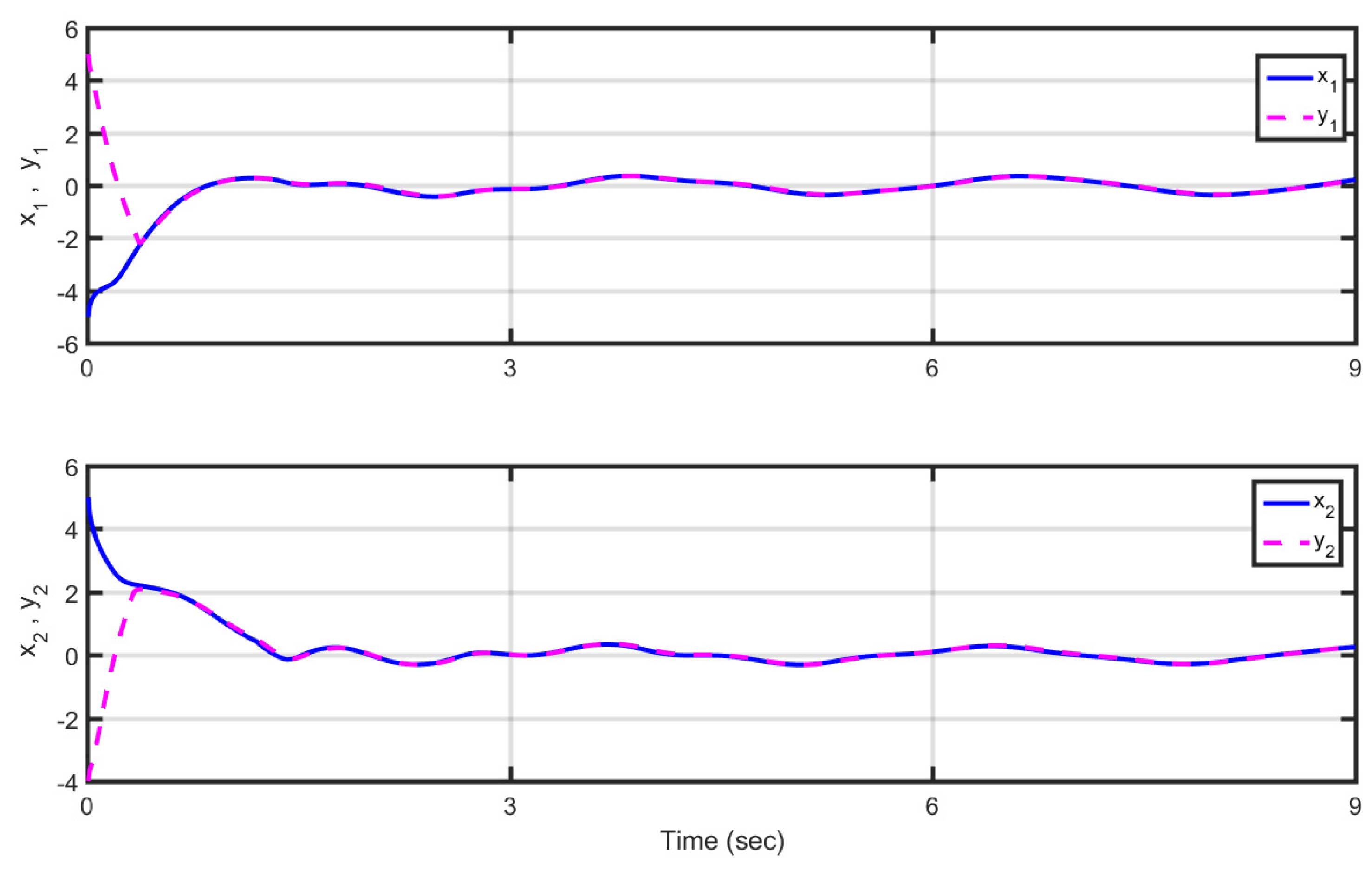
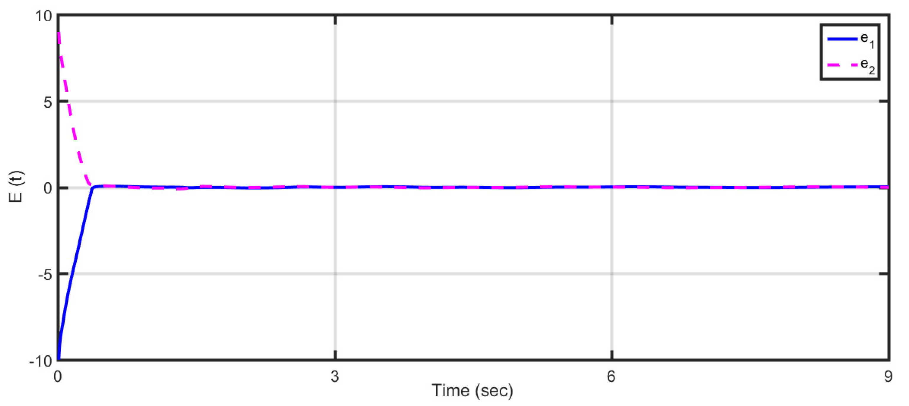
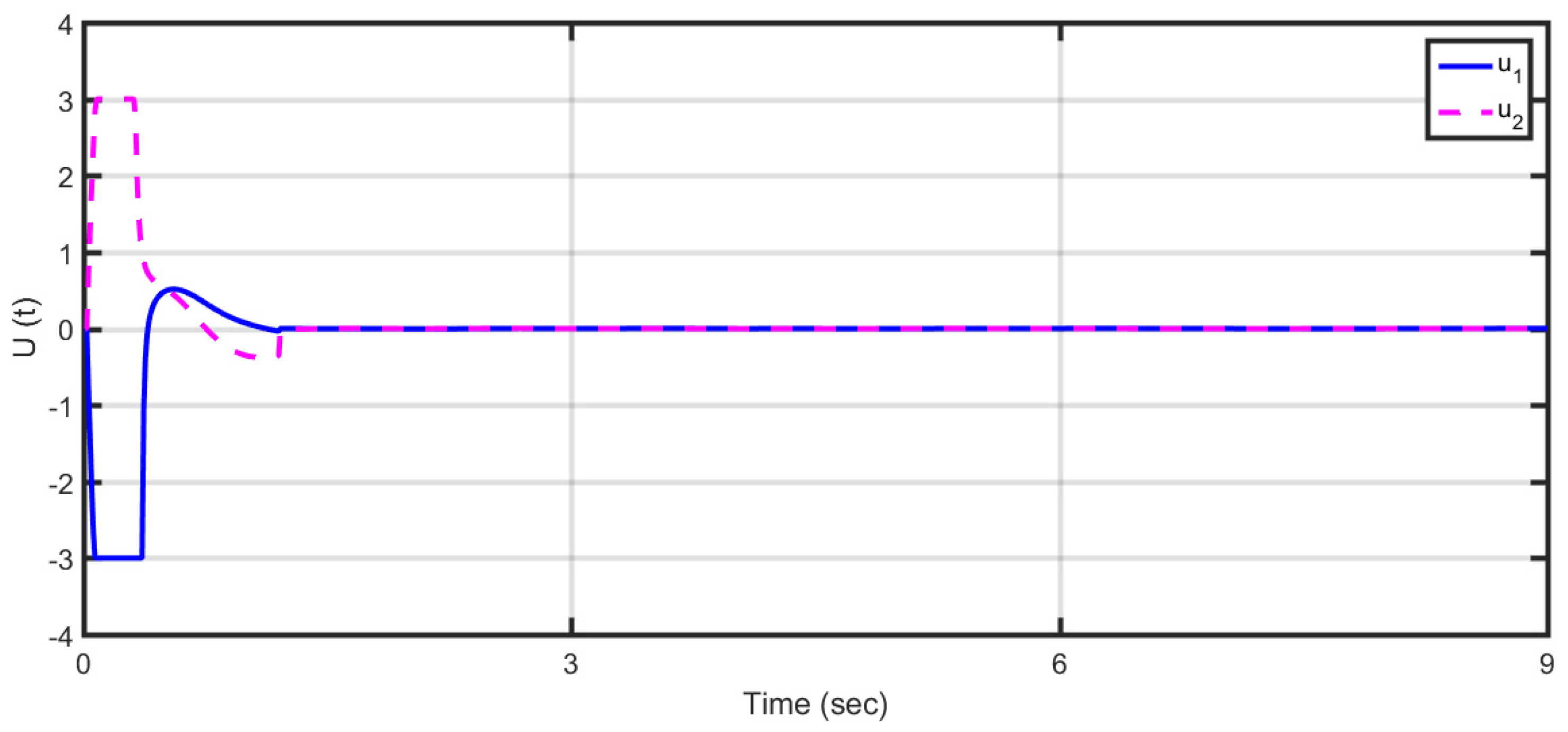
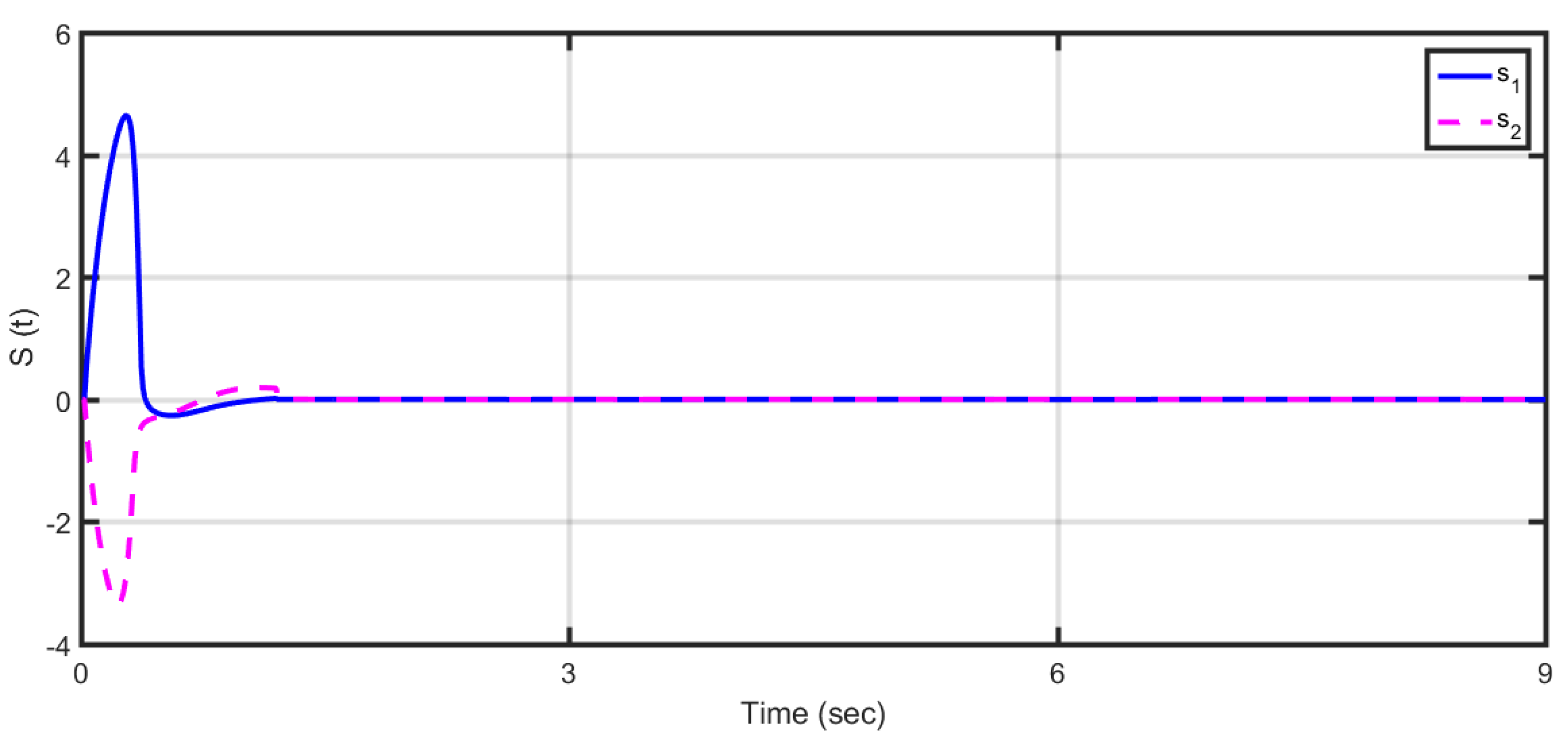
4.1. Synchronization of 2D Unknown Hopfield Delayed FONNSs

In this example, the following 2-dimensional unknown Hopfield delayed FONNSs are considered for illustration. Therefore, the drive system is as follows:
D κ x 1 t = x 1 t 2   t a n h x 1 t + 2.3   t a n h x 2 t 1.3   t a n h x 1 t τ 1.2   t a n h x 2 t τ + 0.2       D κ x 2 t = x 2 t 3.3   t a n h x 1 t 1.5   t a n h x 2 t 3.5   t a n h x 1 t τ 2   t a n h x 2 t τ + 0.3 ,
with κ = 0.92 and τ = 1.2 . Also, x 1 0 = 5 and x 2 0 = 5 are selected as initial values.
And, the response system is as follows:
D κ y 1 t = y 1 t + 0.5   s i n y 1 t + s i n y 2 t + 0.5   t a n h y 1 t τ + t a n h y 2 t τ + 0.1 + Ψ 1 u 1 t           D κ y 2 t = 0.5   y 2 t + s i n y 1 t 0.5   s i n y 2 t 0.5   t a n h y 1 t τ t a n h y 2 t τ + 0.15 + Ψ 2 u 2 t ,
Also, y 1 0 = 5 and y 2 0 = 4 are the initial values.
The parameters of the control technique (37) are fixed as p 1 = p 2 = 3 ,   ν = 2.5 ,   r = 2 ,   l = 1.2 , and z = 1.8 . Moreover, the constants of the sliding surface (24) are selected by μ 1 = μ 2 = 2 , q = 0.9 . Furthermore, the nonlinear function Ψ i u i t is defined as
Ψ i u i t = 3                                                                                 i f   u i t > 3   0.98 u i t                     i f 3 u i t 3   3                                                                                 i f   u i t < 3                       i = 1 ,   2 .
Figure 1 and Figure 2 depict, respectively, the synchronization of the states of FO drive-response mechanisms (52) and (53) and the controlled error of the Hopfield delayed FONNSs ((52) and (53)). Evidently, the unusual attractors of the chaotic FO error system are rapidly stabilized. In addition, Figure 3 depicts the time history of the adaptive controller (37). It is observed that the control input (37) approaches equilibrium without any traces of the chattering phenomena. This indicates that the devised adaptive controller can effectively synchronize the 2-dimensional Hopfield delayed FONNSs ((52) and (53)). Moreover, as shown in Figure 3, as the signals of the control laws method and the saturation boundaries, they are suppressed by the saturation condition, and the leaping phenomena occur. Therefore, jumping states and switching states may be simply applied, particularly when relays and indicated saturation conditions are used.
Also, Figure 4 and Figure 5 show the time response of the sliding surface (24) in both function plot and surface plot, respectively. Clearly, from Figure 4, each parameter of the sliding surface (24) approaches the origin, and there are no traces of the chattering phenomena in the sliding surfaces. In addition, Figure 5 indicates that the result of applying this method is a stable surface.

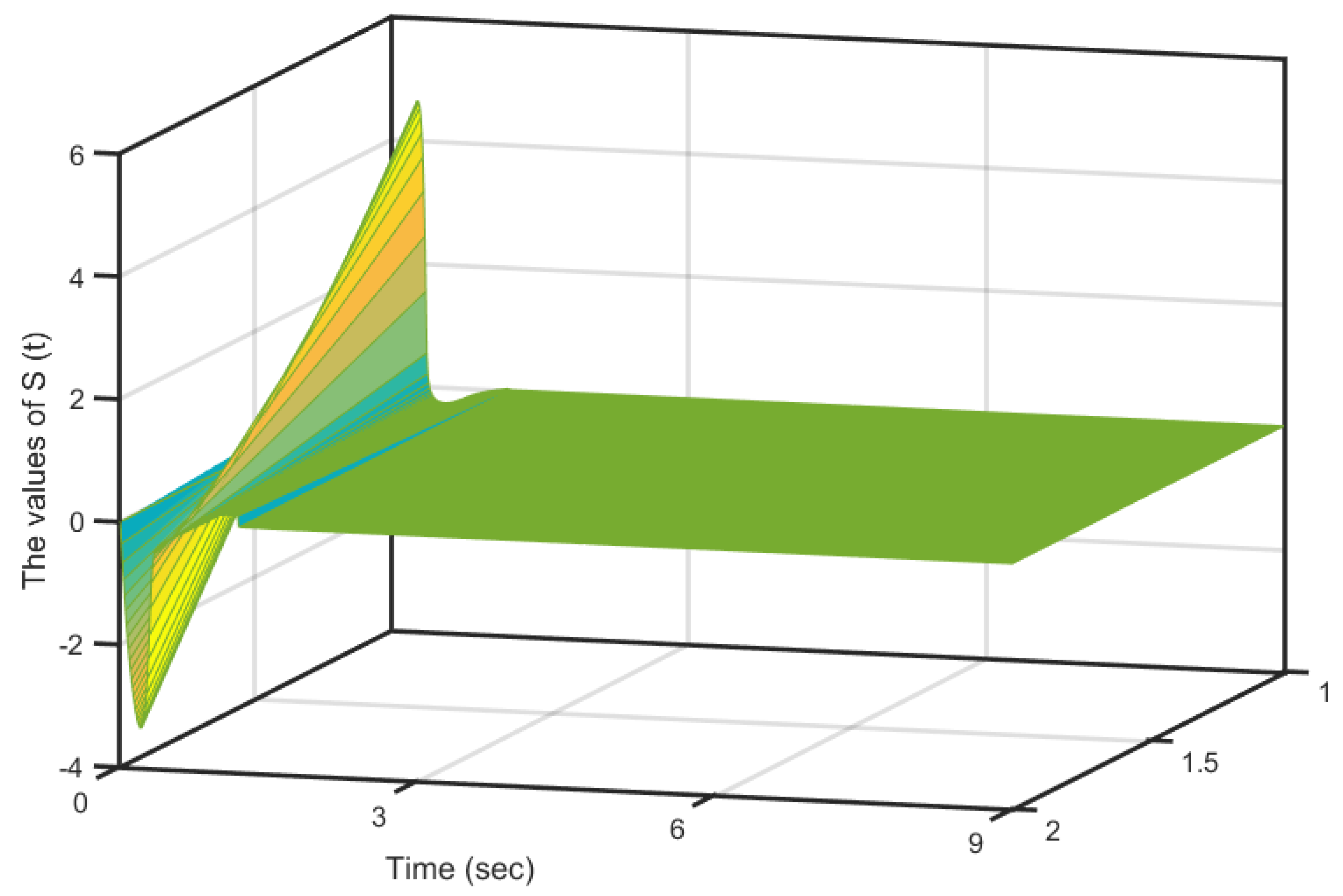
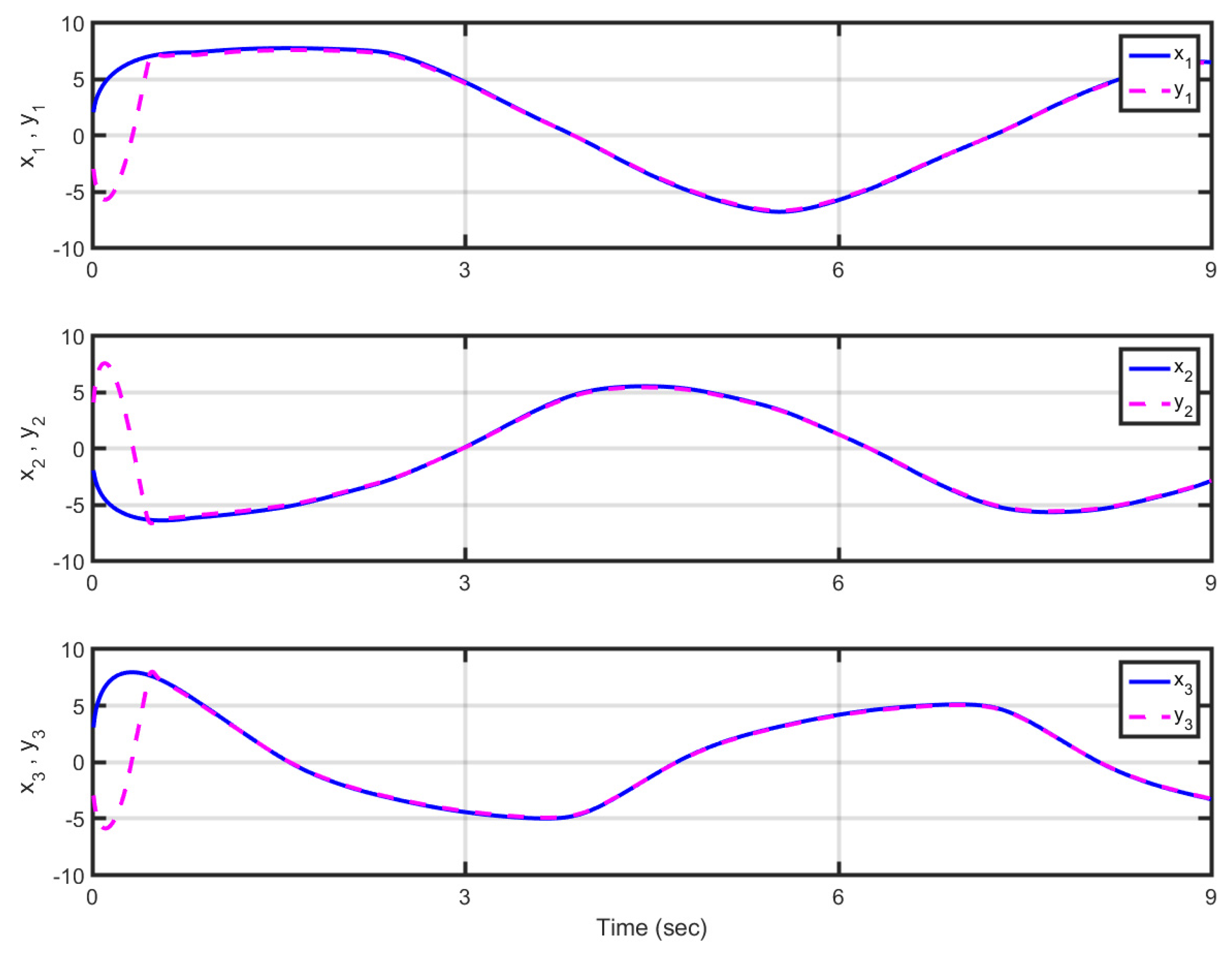
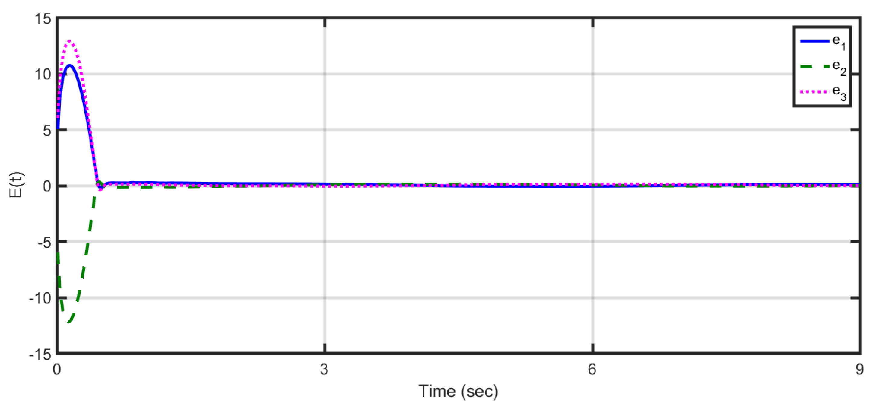
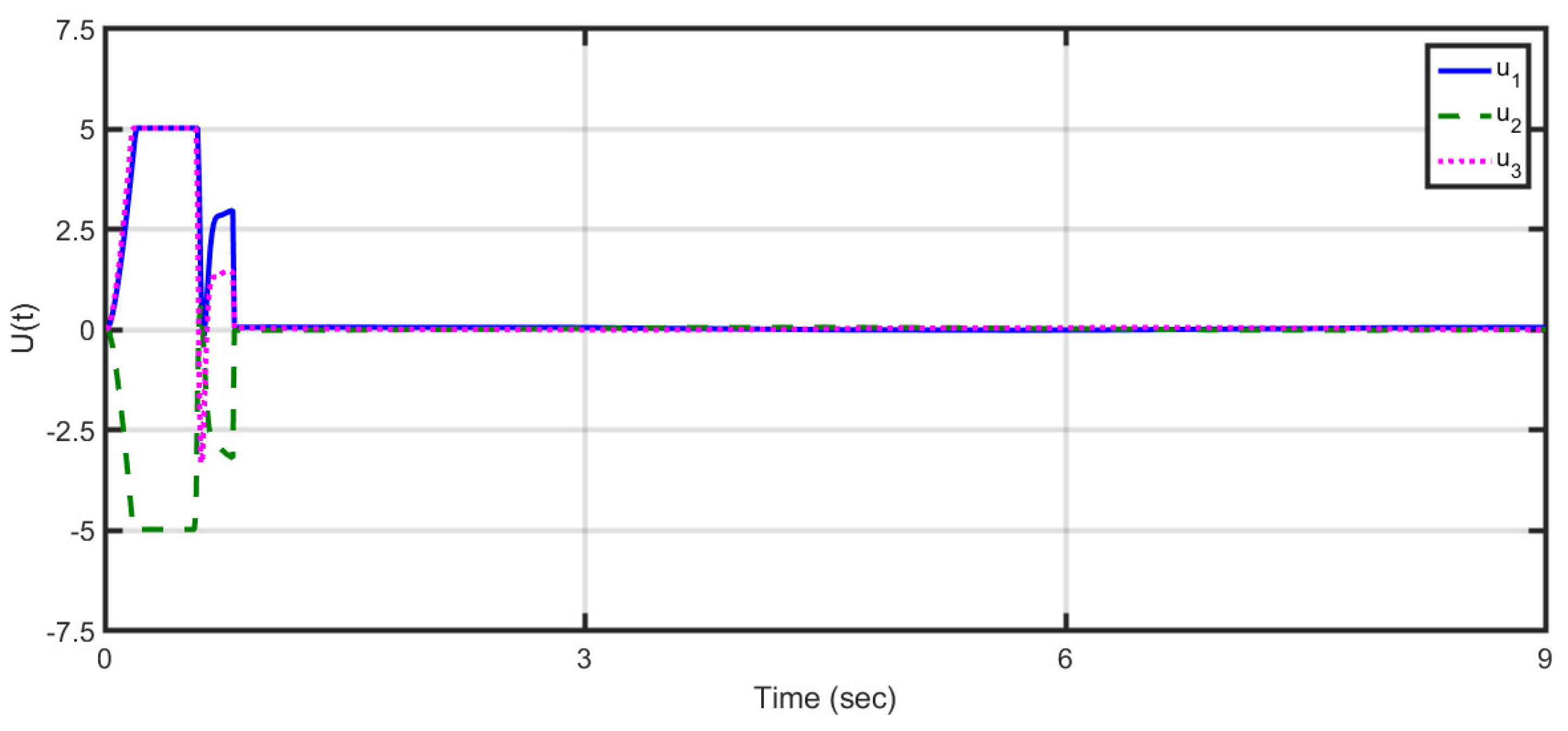
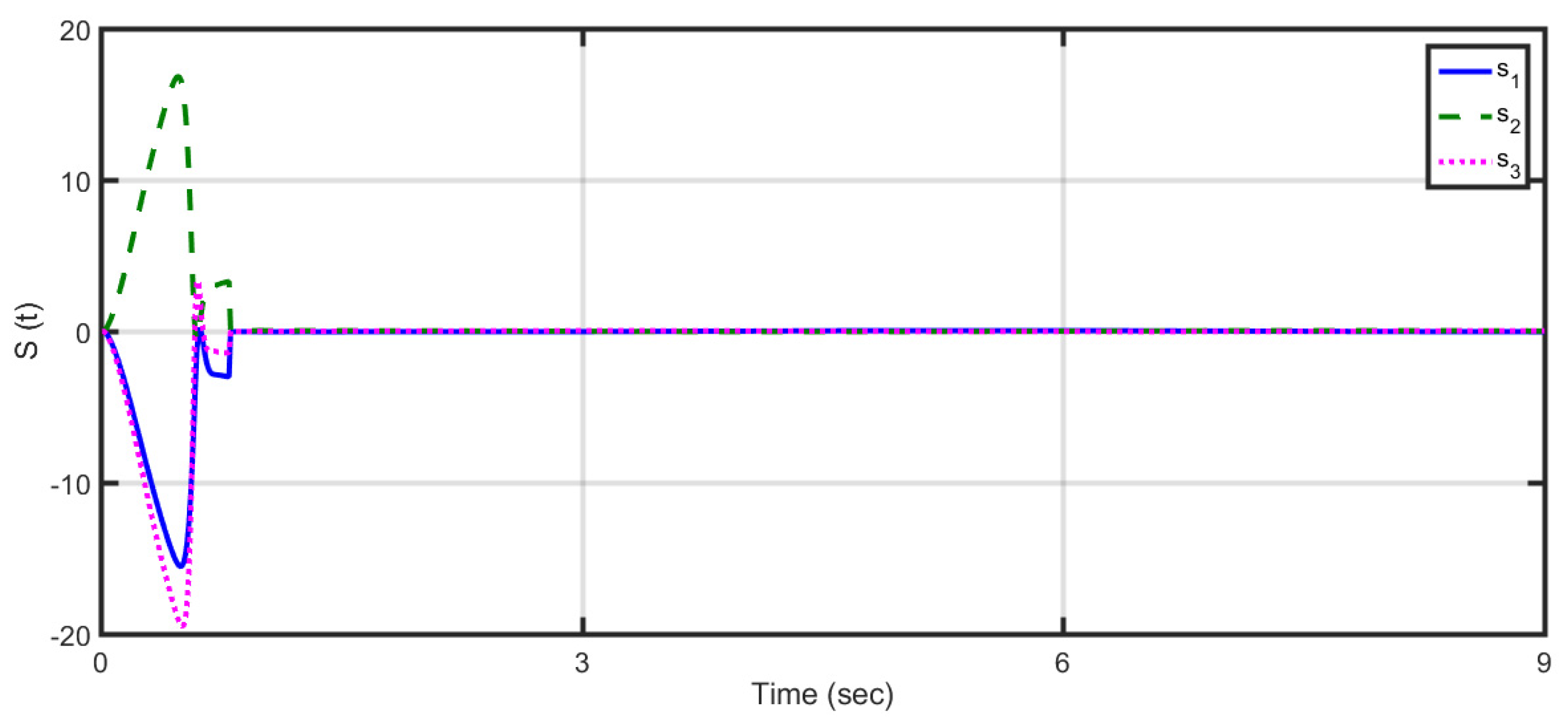
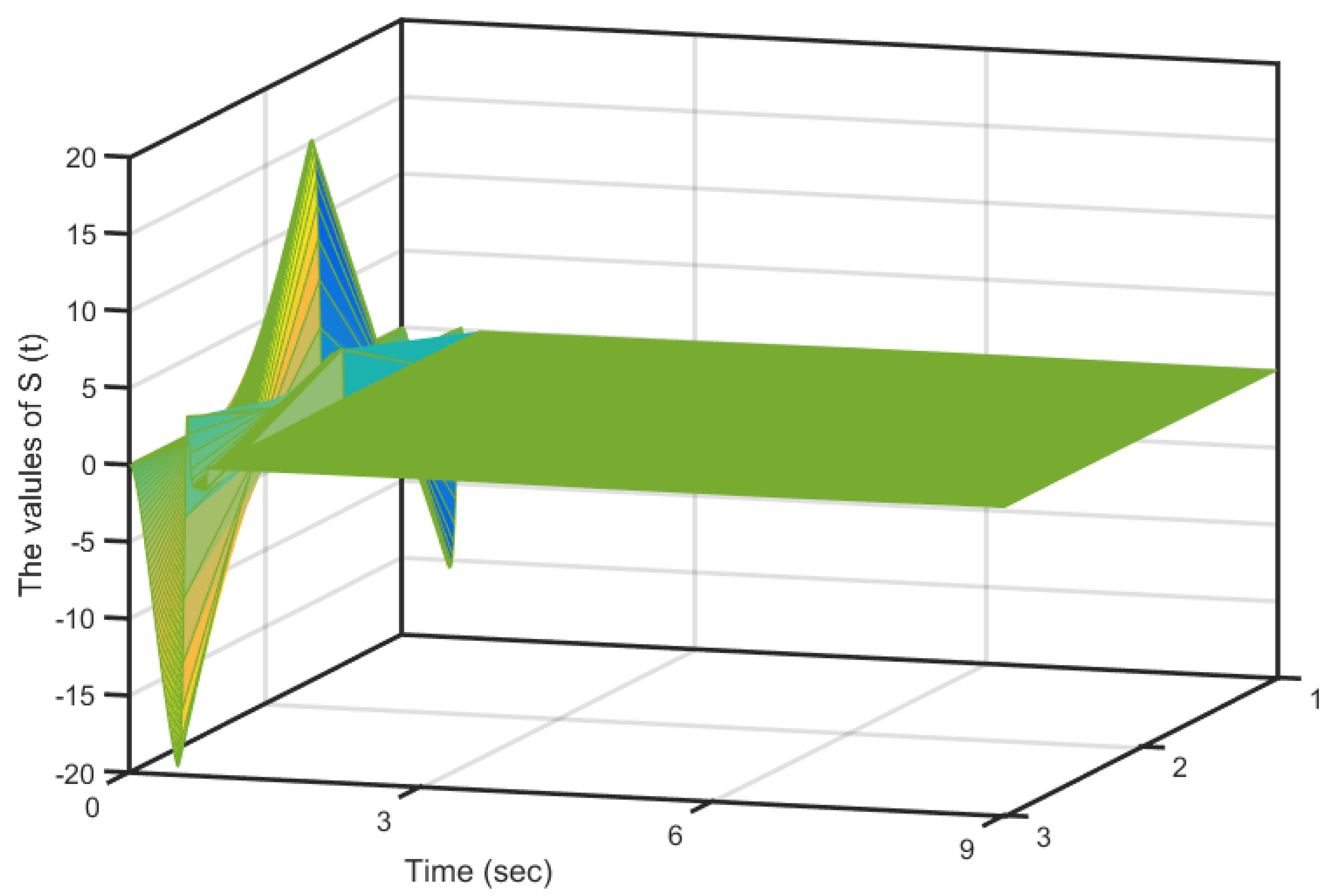
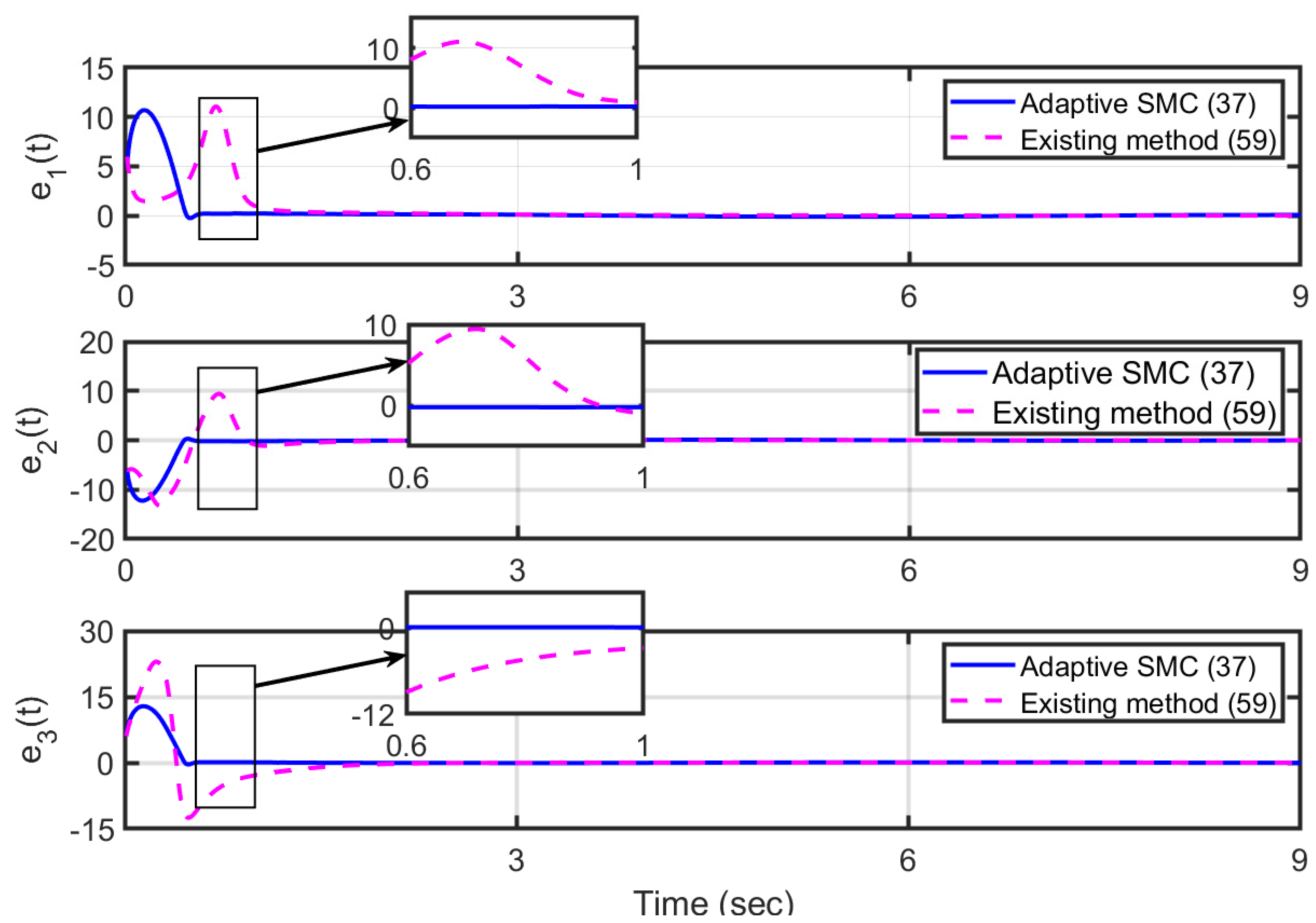
4.2. Synchronization of 3D Unknown Hopfield Delayed FONNSs

Here, to illustrate the effectiveness of the proposed adaptive SMC, 3-dimensional unknown Hopfield delayed FONNSs are investigated. Thus, the drive system is
D κ x 1 t = x 1 t + 2   t a n h x 1 1.2   t a n h x 2 + 1.3   t a n h x 3 t τ + 0.2 ,                                                                                 D κ x 2 t = x 2 t + 1.8   t a n h x 1 + 1.71   t a n h x 2 + 1.15   t a n h x 3 1.3   t a n h x 3 t τ 0.3 , D κ x 3 t = x 3 t 4.75   t a n h x 1 1.1 t a n h x 3 + 0.56   t a n h x 3 t τ ,                                                                                
where κ = 0.96 and τ = 0.8 . Also, x 1 0 = 2 ,   x 2 0 = 2 and x 3 0 = 3 are selected as initial values.
And, the response system is as follows:
D κ y 1 t = 6   y 1 t + 3   s i n y 1 t 2.5   s i n y 3 t + s i n y 2 t τ + 3   t a n h y 3 t τ + 0.5 + Ψ 1 u 1 t ,   D κ y 2 t = 7   y 2 t s i n y 1 t + 1.5 s i n y 2 t + 2 s i n y 3 t t a n h y 1 t τ + 1.6   s i n y 3 t τ                                                                                                                         + 2   t a n h y 3 t τ + 0.1 + Ψ 2 u 2 t , D κ y 3 t = 5.5   y t 3 2.5   s i n y 1 t + 2   s i n y 2 t s i n y 3 t s i n y 2 t τ                                                                                                                         + 3   t a n h y 1 t τ + 0.3 + Ψ 3 u 3 t ,
Also, y 1 0 = 3 , y 2 0 = 4 and y 2 0 = 3 are the initial values.
The constants of the control method (37) are fixed as p 1 = p 2 = 2.5 and p 3 = 4 ,   ν = 3 ,   r = 1.8 ,   l = 2.3 , and z = 2.6 . Plus, the parameters of the SS (24) are μ 1 = 4 , μ i = 2 ,  q = 0.94 and ρ = 5 . Furthermore, the nonlinear mechanism Ψ i u i t is as follows:
Ψ i u i t = 5                         i f   u i t > 5   u i t   i f 5 u i t 5   5                         i f   u i t < 5               i = 1 ,   2,3 .
The synchronized states of the drive-response Hopfield delayed FONNSs ((55) and (56)), as well as the state trajectories of the controlled error of the Hopfield delayed FONNSs, are shown in Figure 6 and Figure 7, respectively. It is clear that the chaotic FO error system’s peculiar attractions are fast stabilizing. In addition, the time history of the adaptive controller (37) is shown in Figure 8. It can be seen that the control input (37) is moving closer and closer to equilibrium without exhibiting any signs of the chattering phenomenon. This indicates that the adaptive controller that was developed is capable of synchronizing the 3-dimensional unknown Hopfield delayed FONNSs ((55) and (56)) in an efficient manner. In addition, as can be seen in Figure 3 that, when the signals of the control law go close to the borders of the saturation state, the saturation condition causes them to be suppressed, which in turn causes the jumping phenomenon to take place. As a direct consequence of this, jumping states and switching states may be implemented with relative ease, in particular in situations where relays and indicated saturation conditions are used.
Furthermore, the temporal response of the SS (24), applied to synchronize the drive-response Hopfield delayed FONNSs ((55) and (56)), is shown in both the function plot and the surface plot, shown in Figure 9 and Figure 10, respectively. Figure 9 makes it abundantly clear that each parameter of the sliding surface (24) is getting closer and closer to the origin, and there are no indications that the chattering phenomenon is present in the sliding surfaces. In addition, the use of this approach results in a surface that is stable, as seen in Figure 10.
Now, to draw a comparison to the adaptive SMC method, we also employ another adaptive sliding mode controller, as outlined in Reference [48], for the synchronization of the FO Hopfield neural network described by Equations (55) and (56) with κ = 0.99 . It is worth noting that Reference [48] deals with adaptive synchronization for a specific category of uncertain delayed fractional-order Hopfield neural networks in the presence of external disturbances. Here, we adopt the control methodology from [48] in the following manner:
s i t = D κ e i ( t ) + p i e i ( t ) + q i   s i g n e i t d t ,
where p i and q i are positive numbers. Also, for i = 1 ,   2 ,   3 :
u i t = a ^ i t + p i e i t d ^ i t s i t j = 1 3 M i j L j f e j t + j = 1 3 P i j L j g e j t τ q i   s i g n e i t                                     ς i a s i t ς i b   s i g n s i t ,
a ^ ˙ i = η i a s i t e i t
d ^ ˙ i = η i d s i t ,        
where L j f ,   L j g , ς i a , ς i b , η i a and η i b are positive constants as control parameters.
The controller parameters are chosen as L 1 f = L 2 f = 2.2 , L 3 f = 2 , L 1 g = L 2 g = L 3 g = 2.3 , ς 1 a = ς 2 a = ς 3 a = 1.9 , ς 1 b = 2.5 , ς 2 b = ς 3 b = 3 , η 1 a = η 2 a = η 3 a = 1.8 , and η 1 b = 2 , η 2 b = η 3 b = 2.5 . Moreover, for i = 1 , 2 , 3 , p i = 0.9 and q i = 1.1 .
Figure 11 illustrates the trajectories of controlled error states for the Hopfield delayed FONNSs described by equations (55) and (56). These systems are controlled using the proposed adaptive SMC method (37) and the SMC method (59) presented in [48]. While both methods manage to guide the error states to the origin, it is evident that the suggested adaptive SMC exhibits superior convergence compared to the SMC method (59). A detailed analysis of this comparison is consolidated in Table 1.
Remark 3.
In Figure 4 and Figure 8, we delve into the concept of sliding surfaces, illustrating the convergence of sliding surface states to the origin. This illustrative model is widely employed across the relevant literature. However, it is important to note that obtaining an exact depiction of the stable surfaces proves challenging due to the nature of Figure 4 and Figure 8, which present line views of sliding surfaces (24) in Scenarios 1 and 2. To address this limitation, we have included Figure 5 and Figure 10, which offer a surface plotting perspective to visually demonstrate the stability of sliding surface (24) in Scenarios 1 and 2. These supplementary figures provide a more comprehensive understanding of the stability concept.
Remark 4.
The dynamic-free adaptive sliding mode control method, rooted in the principles of the frequency distributed model (FDM) theorem, the Lyapunov stability theorem, and norm-bounded control, presents a compelling approach for addressing the synchronization of non-identical systems, all while remaining free from explicit system dynamics. In contrast to traditional methods that often rely on explicit knowledge of system dynamics, the dynamic-free nature of this approach stands out. By capitalizing on the FDM theorem, the method estimates and counteracts disturbances without necessitating in-depth knowledge of the complex underlying dynamics of the systems. This is especially advantageous when dealing with non-identical systems, as such complexities can vary significantly. Furthermore, the inclusion of the Lyapunov stability theorem guarantees the method’s convergence and stability, even in the context of non-identical systems. The controller’s adaptability is further augmented by its adaptive nature, enabling it to automatically adjust control actions based on observed differences between the systems. This adaptability addresses the challenge of synchronizing non-identical systems by ensuring that the control strategy accommodates variations. The norm-bounded control aspect maintains control signals within predefined bounds, resulting in a smoother and more predictable response, which is particularly crucial when dealing with diverse system dynamics. In conclusion, this dynamic-free adaptive sliding mode control method offers a novel and potent solution for synchronizing non-identical systems. By focusing on disturbance estimation, adaptability, and stability analysis, the method overcomes the limitations of explicit system dynamics. This distinctive feature, coupled with its adaptability, positions the method as a strong contender for real-world scenarios involving non-identical systems.
Remark 5.
In practical applications, particularly when dealing with complex fractional-order (FO) systems that defy accurate modeling and are plagued by inherent uncertainties, this model-free controller holds substantial promise. Furthermore, its implementation can be seamlessly achieved using readily available digital devices such as the FPGA (Field-Programmable Gate Array) or DSP (Digital Signal Processing), requiring only knowledge of the system’s current state.
Remark 6.
Research into the proposed dynamic-free adaptive SMC approach for synchronizing delayed fractional-order nonlinear chaotic systems (FONNS) is an evolving area with notable achievements. However, it is essential to acknowledge the existing limitations, with the anticipation of future improvements. These limitations encompass (1) constraints on the differentiation order, typically limited to the range of 0 to 1; (2) the intricate nature of analyzing and computing models for delayed systems and control methodologies, which can be challenging; (3) the reliance on trial-and-error methods for selecting optimal controller settings.
Addressing these restrictions is pivotal for advancing the efficacy and versatility of the dynamic-free adaptive SMC approach in synchronizing chaotic systems.

5. Discussion and Conclusions

This work presents a novel dynamic-free adaptive sliding mode control (adaptive SMC) methodology for achieving synchronization in a specific class of chaotic delayed fractional-order neural network systems with input saturation. By incorporating the FDM and the FO version of the Lyapunov stability theory, the proposed adaptive SMC method effectively overcomes the inherent chaotic behavior exhibited by the delayed FONNSs and ensures synchronization. One key advantage of the approach is the decoupling of control inputs from the nonlinear–linear dynamical terms of the system, leveraging the norm-boundedness property of states in chaotic systems. Through numerical simulations, the effectiveness of the adaptive SMC method has been demonstrated to achieve chaos synchronization in delayed fractional-order Hopfield neural network systems, showcasing its robustness and efficiency. The integration of the FDM and FO Lyapunov stability theorem offers a promising solution for synchronizing chaotic unknown Hopfield delayed FONNSs with input saturation. This innovative approach holds potential applications in diverse domains that require the synchronization of such systems. Therefore, the proposed dynamic-free adaptive SMC method represents a significant contribution to the field of chaotic systems control, providing a reliable and efficient means to achieve synchronization in complex neural network systems with time delays and fractional-order dynamics, even in the presence of input saturation. The findings open up new possibilities for research and applications in various areas where the stable synchronization of chaotic systems is of paramount importance.

Author Contributions

Conceptualization, M.R., C.Z. and A.B.-O.; Methodology, M.R.; Software, M.R. and M.T.; Validation, M.R. and A.B.-O.; Formal analysis, A.B.-O.; Resources, C.Z.; Writing—original draft, M.R.; Writing—review & editing, M.T. and A.B.-O.; Supervision, C.Z.; Funding acquisition, C.Z. All authors have read and agreed to the published version of the manuscript.

Funding

The National Nature Sciences Foundation of China (Grant No.: 12071096) has supported this work.

Data Availability Statement

No new data were created or analyzed in this study. Data sharing is not applicable to this article.

Conflicts of Interest

The authors declare no conflict of interest.

References

  1. Alikhanov, A.A.; Asl, M.S.; Huang, C.; Khibiev, A. A second-order difference scheme for the nonlinear time-fractional diffusion-wave equation with generalized memory kernel in the presence of time delay. J. Comput. Appl. Math. 2023, 438, 115515. [Google Scholar] [CrossRef]
  2. Asl, M.S.; Javidi, M. Novel algorithms to estimate nonlinear FDEs: Applied to fractional order nutrient-phytoplankton–zooplankton system. J. Comput. Appl. Math. 2018, 339, 193–207. [Google Scholar] [CrossRef]
  3. Joshi, M.; Bhosale, S.; Vyawahare, V.A. A survey of fractional calculus applications in artificial neural networks. Artif. Intell. Rev. 2023. [Google Scholar] [CrossRef]
  4. Kathamuthu, N.D.; Subramaniam, S.; Le, Q.H.; Muthusamy, S.; Panchal, H.; Sundararajan, S.C.M.; Alrubaie, A.J.; Zahra, M.M.A. A deep transfer learning-based convolution neural network model for COVID-19 detection using computed tomography scan images for medical applications. Adv. Eng. Softw. 2023, 175, 103317. [Google Scholar] [CrossRef]
  5. Sharma, M.; Pant, S.; Yadav, P.; Sharma, D.K.; Gupta, N.; Srivastava, G. Advancing Security in the Industrial Internet of Things Using Deep Progressive Neural Networks. Mob. Netw. Appl. 2023. [Google Scholar] [CrossRef]
  6. Moon, S.; Hou, L.; Han, S. Empirical study of an artificial neural network for a manufacturing production operation. Oper. Manag. Res. 2023, 16, 311–323. [Google Scholar] [CrossRef]
  7. Xiang, L.; Gai, J.; Bao, Y.; Yu, J.; Schnable, P.S.; Tang, L. Field-based robotic leaf angle detection and characterization of maize plants using stereo vision and deep convolutional neural networks. J. Field Robot. 2023, 40, 1034–1053. [Google Scholar] [CrossRef]
  8. Roohi, M.; Zhang, C.; Chen, Y. Adaptive model-free synchronization of different fractional-order neural networks with an application in cryptography. Nonlinear Dyn. 2020, 100, 3979–4001. [Google Scholar] [CrossRef]
  9. Solak, M.; Faydasicok, O.; Arik, S. A general framework for robust stability analysis of neural networks with discrete time delays. Neural Netw. 2023, 162, 186–198. [Google Scholar] [CrossRef]
  10. Nagamani, G.; Adhira, B.; Soundararajan, G. Non-fragile extended dissipative state estimation for delayed discrete-time neural networks: Application to quadruple tank process model. Nonlinear Dyn. 2021, 104, 451–466. [Google Scholar] [CrossRef]
  11. Kiruthika, R.; Krishnasamy, R.; Lakshmanan, S.; Prakash, M.; Manivannan, A. Non-fragile sampled-data control for synchronization of chaotic fractional-order delayed neural networks via LMI approach. Chaos Solitons Fractals 2023, 169, 113252. [Google Scholar] [CrossRef]
  12. Zhou, W.; Zhou, X.; Yang, J.; Zhou, J.; Tong, D. Stability Analysis and Application for Delayed Neural Networks Driven by Fractional Brownian Noise. IEEE Trans. Neural Netw. Learn. Syst. 2018, 29, 1491–1502. [Google Scholar] [CrossRef] [PubMed]
  13. Wang, Y.; Zhu, S.; Shao, H.; Feng, Y.; Wang, L.; Wen, S. Comprehensive analysis of fixed-time stability and energy cost for delay neural networks. Neural Netw. 2022, 155, 413–421. [Google Scholar] [CrossRef] [PubMed]
  14. Ramajayam, S.; Rajavel, S.; Samidurai, R.; Cao, Y. Finite-Time Synchronization for T–S Fuzzy Complex-Valued Inertial Delayed Neural Networks Via Decomposition Approach. Neural Process. Lett. 2023. [Google Scholar] [CrossRef]
  15. Nancy Jane, Y.; Khanna Nehemiah, H.; Arputharaj, K. A Q-backpropagated time delay neural network for diagnosing severity of gait disturbances in Parkinson’s disease. J. Biomed. Inform. 2016, 60, 169–176. [Google Scholar] [CrossRef]
  16. Rasooli Berardehi, Z.; Zhang, C.; Taheri, M.; Roohi, M.; Khooban, M.H. Implementation of T-S fuzzy approach for the synchronization and stabilization of non-integer-order complex systems with input saturation at a guaranteed cost. Trans. Inst. Meas. Control 2023, 45, 2536–2553. [Google Scholar] [CrossRef]
  17. Rasooli Berardehi, Z.; Zhang, C.; Taheri, M.; Roohi, M.; Khooban, M.H. A Fuzzy Control Strategy to Synchronize Fractional-Order Nonlinear Systems Including Input Saturation. Int. J. Intell. Syst. 2023, 2023, 1550256. [Google Scholar] [CrossRef]
  18. Shalaby, R.; El-Hossainy, M.; Abo-Zalam, B.; Mahmoud, T.A. Optimal fractional-order PID controller based on fractional-order actor-critic algorithm. Neural Comput. Appl. 2023, 35, 2347–2380. [Google Scholar] [CrossRef]
  19. Farid, Y.; Ruggiero, F. Finite-time extended state observer and fractional-order sliding mode controller for impulsive hybrid port-Hamiltonian systems with input delay and actuators saturation: Application to ball-juggler robots. Mech. Mach. Theory 2022, 167, 104577. [Google Scholar] [CrossRef]
  20. Xing, Y.; Wang, Y. Finite-Time Adaptive NN Backstepping Dynamic Surface Control for Input-Delay Fractional-Order Nonlinear Systems. IEEE Access 2023, 11, 5206–5214. [Google Scholar] [CrossRef]
  21. Taheri, M.; Chen, Y.; Zhang, C.; Berardehi, Z.R.; Roohi, M.; Khooban, M.H. A finite-time sliding mode control technique for synchronization chaotic fractional-order laser systems with application on encryption of color images. Optik 2023, 285, 170948. [Google Scholar] [CrossRef]
  22. Taheri, M.; Zhang, C.; Berardehi, Z.R.; Chen, Y.; Roohi, M. No-chatter model-free sliding mode control for synchronization of chaotic fractional-order systems with application in image encryption. Multimed. Tools Appl. 2022, 81, 24167–24197. [Google Scholar] [CrossRef]
  23. El-Sousy, F.F.M.; Alqahtani, M.H.; Aljumah, A.S.; Aly, M.; Almutairi, S.Z.; Mohamed, E.A. Design Optimization of Improved Fractional-Order Cascaded Frequency Controllers for Electric Vehicles and Electrical Power Grids Utilizing Renewable Energy Sources. Fractal Fract. 2023, 7, 603. [Google Scholar] [CrossRef]
  24. Drakunov, S.V.; Utkin, V.I. Sliding mode control in dynamic systems. Int. J. Control 1992, 55, 1029–1037. [Google Scholar] [CrossRef]
  25. Jia, T.; Chen, X.; He, L.; Zhao, F.; Qiu, J. Finite-Time Synchronization of Uncertain Fractional-Order Delayed Memristive Neural Networks via Adaptive Sliding Mode Control and Its Application. Fractal Fract. 2022, 6, 502. [Google Scholar] [CrossRef]
  26. Karimaghaee, P.; Rashidnejad Heydari, Z. Lag-synchronization of two different fractional-order time-delayed chaotic systems using fractional adaptive sliding mode controller. Int. J. Dyn. Control 2021, 9, 211–224. [Google Scholar] [CrossRef]
  27. Zhang, H.; Yan, Y.; Mu, Y.; Ming, Z. Neural Network-Based Adaptive Sliding-Mode Control for Fractional Order Fuzzy System With Unmatched Disturbances and Time-Varying Delays. IEEE Trans. Syst. Man Cybern. Syst. 2023, 53, 5174–5184. [Google Scholar] [CrossRef]
  28. Shi, X.; Jin, Y.; Zhou, X.; Wang, C. Sliding mode control for fractional-order time-varying delay systems under external excitation. J. Vib. Control 2022, 29, 1713–1725. [Google Scholar] [CrossRef]
  29. Chen, J.; Li, C.; Yang, X. Global Mittag–Leffler projective synchronization of nonidentical fractional-order neural networks with delay via sliding mode control. Neurocomputing 2018, 313, 324–332. [Google Scholar] [CrossRef]
  30. Song, X.; Song, S.; Li, B.; Tejado Balsera, I. Adaptive projective synchronization for time-delayed fractional-order neural networks with uncertain parameters and its application in secure communications. Trans. Inst. Meas. Control 2017, 40, 3078–3087. [Google Scholar] [CrossRef]
  31. Bahraini, M.S.; Mahmoodabadi, M.J.; Lohse, N. Robust Adaptive Fuzzy Fractional Control for Nonlinear Chaotic Systems with Uncertainties. Fractal Fract. 2023, 7, 484. [Google Scholar] [CrossRef]
  32. Thuan, M.V.; Huong, D.C. Robust guaranteed cost control for time-delay fractional-order neural networks systems. Optim. Control Appl. Methods 2019, 40, 613–625. [Google Scholar] [CrossRef]
  33. Dalir, M.; Bigdeli, N. An Adaptive neuro-fuzzy backstepping sliding mode controller for finite time stabilization of fractional-order uncertain chaotic systems with time-varying delays. Int. J. Mach. Learn. Cybern. 2021, 12, 1949–1971. [Google Scholar] [CrossRef]
  34. Yan, Y.; Zhang, H.; Sun, J.; Wang, Y. Sliding Mode Control Based on Reinforcement Learning for T-S Fuzzy Fractional-Order Multiagent System With Time-Varying Delays. IEEE Trans. Neural Netw. Learn. Syst. 2023, 1–12. [Google Scholar] [CrossRef]
  35. Yang, F.; Shen, Y.; Li, D.; Lin, S.; Muyeen, S.M.; Zhai, H.; Zhao, J. Fractional-Order Sliding Mode Load Frequency Control and Stability Analysis for Interconnected Power Systems With Time-Varying Delay. IEEE Trans. Power Syst. 2023, 1–11. [Google Scholar] [CrossRef]
  36. Gu, Y.; Sun, J.; Fu, X. A Novel Robust Neural Network Sliding-Mode Control Method for Synchronizing Fractional Order Chaotic Systems in the Presence of Uncertainty, Disturbance and Time-Varying Delay. J. Electr. Eng. Technol. 2023, 18, 1325–1335. [Google Scholar] [CrossRef]
  37. Parvizian, M.; Khandani, K.; Majd, V.J. A non-fragile observer-based adaptive sliding mode control for fractional-order Markovian jump systems with time delay and input nonlinearity. Trans. Inst. Meas. Control 2020, 42, 1448–1460. [Google Scholar] [CrossRef]
  38. Podlubny, I. Fractional Differential Equations: An Introduction to Fractional Derivatives, Fractional Differential Equations, to Methods of Their Solution and Some of Their Applications; Elsevier Science: Amsterdam, The Netherlands, 1998. [Google Scholar]
  39. Li, C.; Deng, W. Remarks on fractional derivatives. Appl. Math. Comput. 2007, 187, 777–784. [Google Scholar] [CrossRef]
  40. Li, Y.; Chen, Y.; Podlubny, I. Stability of fractional-order nonlinear dynamic systems: Lyapunov direct method and generalized Mittag–Leffler stability. Comput. Math. Appl. 2010, 59, 1810–1821. [Google Scholar] [CrossRef]
  41. Aguila-Camacho, N.; Duarte-Mermoud, M.A.; Gallegos, J.A. Lyapunov functions for fractional order systems. Commun. Nonlinear Sci. Numer. Simul. 2014, 19, 2951–2957. [Google Scholar] [CrossRef]
  42. Wang, B.; Ding, J.; Wu, F.; Zhu, D. Robust finite-time control of fractional-order nonlinear systems via frequency distributed model. Nonlinear Dyn. 2016, 85, 2133–2142. [Google Scholar] [CrossRef]
  43. Zhang, S.; Yu, Y.; Wang, H. Mittag-Leffler stability of fractional-order Hopfield neural networks. Nonlinear Anal. Hybrid Syst. 2015, 16, 104–121. [Google Scholar] [CrossRef]
  44. Curran, P.F.; Chua, L.O. Absolute Stability Theory and the Synchronization Problem. Int. J. Bifurc. Chaos 1997, 07, 1375–1382. [Google Scholar] [CrossRef]
  45. Roohi, M.; Aghababa, M.P.; Haghighi, A.R. Switching adaptive controllers to control fractional-order complex systems with unknown structure and input nonlinearities. Complexity 2015, 21, 211–223. [Google Scholar] [CrossRef]
  46. Zhang, W.; Xu, D.; Jiang, B.; Pan, T. Prescribed performance based model-free adaptive sliding mode constrained control for a class of nonlinear systems. Inf. Sci. 2021, 544, 97–116. [Google Scholar] [CrossRef]
  47. Asl, M.S.; Javidi, M. An improved PC scheme for nonlinear fractional differential equations: Error and stability analysis. J. Comput. Appl. Math. 2017, 324, 101–117. [Google Scholar] [CrossRef]
  48. Meng, B.; Wang, X. Adaptive Synchronization for Uncertain Delayed Fractional-Order Hopfield Neural Networks via Fractional-Order Sliding Mode Control. Math. Probl. Eng. 2018, 2018, 1603629. [Google Scholar] [CrossRef]
Figure 1. The time evolution of the synchronization of the Hopfield delayed FONNSs ((52) and (53)).
Fractalfract 07 00682 g001
Figure 2. The time evolution of the synchronization errors of the Hopfield delayed FONNSs ((52) and (53)).
Fractalfract 07 00682 g002
Figure 3. The time evolution of the control inputs (37) for the synchronized Hopfield delayed FONNSs ((52) and (53)).
Fractalfract 07 00682 g003
Figure 4. The time evolution of the SS (24) to synchronize the Hopfield delayed FONNSs ((52) and (53)).
Fractalfract 07 00682 g004
Figure 5. The time evolution of the surface plot depicting the SS (24) implementation for achieving synchronization of the Hopfield delayed FONNSs ((52) and (53)).
Fractalfract 07 00682 g005
Figure 6. The evolution of the synchronization of the Hopfield delayed FONNSs ((55) and (56)).
Fractalfract 07 00682 g006
Figure 7. The time evolution of the synchronization error of the Hopfield delayed FONNSs ((55) and (56)).
Fractalfract 07 00682 g007
Figure 8. The time evolution of the control inputs (37) for the synchronized Hopfield delayed FONNSs ((55) and (56)).
Fractalfract 07 00682 g008
Figure 9. The time evolution of the SS (27) to synchronize Hopfield delayed FONNSs ((55) and (56)).
Fractalfract 07 00682 g009
Figure 10. The time evolution of the surface plot depicting the SS (24) implementation for achieving synchronization of the delayed FONNSs ((55) and (56)).
Fractalfract 07 00682 g010
Figure 11. Comparison of state trajectories of the error of the FO systems ((55) and (56)), controlled with suggested adaptive SMC and SMC method in [48].
Fractalfract 07 00682 g011
Table 1. A Comparative Analysis of the Outcomes Achieved with AMF (21) and SMC (37).
Aspects of ComparisonThe Outcomes of This ResearchThe Outcomes of Ref. [48]
Control ApproachDynamic-free adaptive SMCAdaptive SMC
Controller Configuration ParametersIn total, the selection of 2n + 5 parameters is necessary.In total, the selection of 8n parameters is necessary
System Details.The dynamic-free adaptive SMC method does not require dynamic terms of the systems; only the states are sufficient.The Adaptive SMC requires complete access to dynamic terms from both the drive and response systems.
Amplitude of OscillationsStandard Range (determined by the behavior of the error system)Beyond Range (determined by the behavior of the error system)
ConclusionsThe benefits of the suggested dynamic-free adaptive SMC are as follows:
(1) Enhanced robustness;
(2) Simplified controller design for practical feasibility;
(3) Absence of chattering;
(4) Heightened convergence precision.
The advantages of the adaptive SMC method include:
(1) A potential challenge with numerous parameters that can be complex to manage;
(2) Effective operation when the system states are known;
(3) Absence of chattering;
Disclaimer/Publisher’s Note: The statements, opinions and data contained in all publications are solely those of the individual author(s) and contributor(s) and not of MDPI and/or the editor(s). MDPI and/or the editor(s) disclaim responsibility for any injury to people or property resulting from any ideas, methods, instructions or products referred to in the content.

