Derivative-Free Conformable Iterative Methods for Solving Nonlinear Equations

Abstract

In this manuscript, we use approximations of conformable derivatives for designing iterative methods to solve nonlinear algebraic or trascendental equations. We adapt the approximation of conformable derivatives in order to design conformable derivative-free iterative schemes to solve nonlinear equations: Steffensen and Secant-type methods. To our knowledge, these are the first conformable derivative-free schemes in the literature, where the Steffensen conformable method is also optimal; moreover, the Secant conformable scheme is also a procedure with memory. A convergence analysis is made, preserving the order of classical cases, and the numerical performance is studied in order to confirm the theoretical results. It is shown that these methods can present some numerical advantages versus their classical partners, with wide sets of converging initial estimations.

1. Introduction

Many theoretical and applied problems require us to find the solution $\overline{x}\in \mathbb{R}$ of the nonlinear equation $f\left(x\right)=0$, where $f:I\subseteq \mathbb{R}\to \mathbb{R}$. Due to most of the nonlinear problems not having an analytical solution, many authors have proposed numerical methods by means of fixed point schemes to approximate the solution of $\overline{x}$. Most of these procedures possess the evaluation of an integer order derivative, or its approximation.

In the recent literature, some authors have introduced several numerical methods with noninteger order derivatives (fractal derivative, fractional derivative, and conformable derivative). These derivatives of order $\alpha \in (0,1]$ establish a generalization of a classical one, which is a particular case when the order is $\alpha =1$. Noninteger derivatives can be used to model many applied problems because of the higher degree of freedom of its tools compared to classical calculus tools [1,2,3,4].

In Ref. [5], the first Newton’s methods with fractal derivatives are presented, whose order of convergence is quadratic. With regard to iterative schemes with fractional derivatives, the authors in Ref. [6] designed Newton-type methods, of order $2\alpha$, with Caputo and Riemann–Liouville fractional derivatives. In Ref. [7], two Newton’s methods with Caputo and Riemann–Liouville fractional derivatives, of order $\alpha +1$, allow the design of two Traub’s methods with Caputo and Riemann–Liouville fractional derivatives, of order $2\alpha +1$ for each one; these are the first multipoint fractional methods in the literature. The authors in Ref. [8] perform a dynamical analysis of Newton-type methods whose derivatives are replaced by Caputo and Riemann–Liouville fractional derivatives. In Ref. [9], Newton’s schemes with Caputo and Riemann–Liouville fractional derivatives of order $2\alpha$ are proposed, obtaining a quadratic order of convergence in both cases. Also, the authors in Ref. [10] study the dynamics of a family of procedures with Caputo and conformable derivatives of order three.

Iterative methods with fractional derivatives do not hold the order of convergence of their classical versions; they need higher-order fractional derivatives to increase the order of convergence, preventing it from being possible to obtain optimal order procedures according to Kung and Traub conjecture [11]; unlike schemes with conformable derivatives. So, another approach is the conformable calculus [12,13], whose low computational cost constitutes an advantage versus fractional calculus, due to special functions as Gamma or Mittag–Leffler functions are not evaluated [3]. In that sense, several conformable iterative schemes were designed: In Refs. [14,15] are proposed the scalar and vectorial versions of a Newton-type method with conformable derivative/Jacobian, respectively, and a general technique is designed in Ref. [16] in order to obtain the conformable version of any scalar classical procedure. Also, the authors in Ref. [17] proposed the first multipoint conformable method for solving nonlinear systems (a Traub-type method). Finally, some derivative-free schemes were designed (a Steffensen-type and Secant-type procedures) with an approximation of conformable derivatives in Ref. [18], and a Traub–Steffensen-type method in Ref. [19] (in scalar and vectorial version). The theoretical convergence order of these methods is preserved in practice. Indeed, these methods show good qualitative behavior, improving even their respective classical cases in some numerical aspects.

Most of these fractal, fractional, and conformable schemes mentioned above need the evaluation of fractal, fractional, or conformable derivatives, respectively. Since conformable procedures have presented many advantages versus fractional ones, in this manuscript, we focus in the approximation of conformable derivatives in order to design, to our knowledge, the first conformable derivative-free iterative methods to solve nonlinear equations: a Steffensen-type method and a Secant-type method (based in Ref. [18]); we also compare them with their classical partners.

Let us recall some basic definitions from conformable calculus: Given a function $f:[a,\infty )\to \mathbb{R}$, its left conformable derivative, starting from a, of order $\alpha \in (0,1]$, where $a,\alpha ,x\in \mathbb{R}$, being $x>a$, can be defined as shown next [12,13]

$$\left(T_{\alpha }^{a}f\right)\left(x\right)=\underset{\epsilon \to 0}{lim}{\displaystyle \frac{f(x+\epsilon {(x-a)}^{1-\alpha })-f\left(x\right)}{\epsilon }}.$$

(1)

If this limit does exist, then f is $\alpha$-differentiable. Let us suppose that f is differentiable, then $\left(T_{\alpha }^{a}f\right)\left(x\right)=f^{\prime }\left(x\right){(x-a)}^{1-\alpha }$. Given $b\in \mathbb{R}$ such that f is $\alpha$-differentiable in $(a,b)$, then $\left(T_{\alpha }^{a}f\right)\left(a\right)={lim}_{x\to a^{+}}\left(T_{\alpha }^{a}f\right)\left(x\right)$.

This derivative preserves the property of non fractional derivatives: $T_{\alpha }^{a}K=0$, where K is a constant. As mentioned before, this kind of derivative does not require to evaluate any special function.

In Ref. [20], an appropriate conformable Taylor series is provided, as shown in the following result.

Theorem 1 

(Theorem 4.1, [20]). Let $f\left(x\right)$ be an infinitely α-differentiable function, $\alpha \in (0,1]$, about $a_1$, where the conformable derivatives start at a. Then, the conformable Taylor series of $f\left(x\right)$ can be given by

$$f\left(x\right)=f\left(a_1\right)+{\displaystyle \frac{\left(T_{\alpha }^{a}f\right)\left(a_1\right)}{\alpha }}{\delta }_1+{\displaystyle \frac{{\left(T_{\alpha }^{a}f\right)}^{\left(2\right)}\left(a_1\right)}{2{\alpha }^2}}{\delta }_2+R_2(x,a_1,a),$$

(2)

being $L=a_1-a$, $H=x-a$, ${\delta }_1=H^{\alpha }-L^{\alpha }$, ${\delta }_2=H^{2\alpha }-L^{2\alpha }-2L^{\alpha }{\delta }_1$, ….

We can easily prove that ${\delta }_2={\delta }_1^2$, ${\delta }_3={\delta }_1^3$, and so on. So, (2) is expressed as

$$f\left(x\right)=f\left(a_1\right)+{\displaystyle \frac{1}{\alpha }}\left(T_{\alpha }^{a}f\right)\left(a_1\right){\delta }_1+{\displaystyle \frac{1}{2{\alpha }^2}}{\left(T_{\alpha }^{a}f\right)}^{\left(2\right)}\left(a_1\right){\delta }_1^2+R_2(x,a_1,a).$$

(3)

Since the Secant-type method we propose includes memory, we need to introduce a generalization of order of convergence (The R-order [21,22]), but first, let us see the concept of R-factor:

Definition 1 

([21,22]). Let ϕ be a converging iterative method to some limit β, and let $\left\{x_k\right\}$ be an arbitrary sequence in ${\mathbb{R}}^n$ converging to β. Then, the R-factor of the sequence $\left\{x_k\right\}$ is

$$R_m\left(x\right)=\left\{\begin{array}{cc}{\displaystyle lim\underset{k\to \infty }{sup}\left|\right|x_k-\beta {\left|\right|}^{1/k},}\hfill & form=1,\hfill \\ {\displaystyle lim\underset{k\to \infty }{sup}\left|\right|x_k-\beta {\left|\right|}^{1/m^k},}\hfill & form>1.\hfill \end{array}\right.$$

(4)

We can define now the R-order:

Definition 2 

([21,22]). The R-order of convergence of an iterative method ϕ at the point β is

$$O_R(\varphi ,\beta )=\left\{\begin{array}{c}+\infty ,if{R}_m(\varphi ,\beta )=0\forall m\in [1,+\infty ),\hfill \\ inf\{m\in [1,+\infty ):R_m(\varphi ,\beta )=1\},\mathit{in}\mathit{other}\mathit{case}.\hfill \end{array}\right.$$

(5)

The following result states a relation between the roots of a characteristic polynomial and the R-order of an iterative procedure with memory:

Theorem 2 

([21,22]). Let ϕ be an iterative method with memory generating the sequence $\left\{x_k\right\}$ of approximations of the root $\overline{x}$, and let us suppose that the sequence $\left\{x_k\right\}$ converges to $\overline{x}$. If exists a not null constant η, and nonnegative numbers $t_i$, $i\in [0,m]$, such that

$$|e_{k+1}|\le \eta \prod _{i=0}^m{\left|e_{k-i}\right|}^{t_i},$$

is fulfilled, then the R-order of iterative scheme ϕ satisfies

$$O_R(\varphi ,\overline{x})\ge s^{*},$$

being $s^{*}$ the only positive root of polynomial

$$s^{m+1}-\sum _{i=0}^m{t}_i{s}^{m-i}=0.$$

(6)

Finally, if we take into account that, given an iteration function $\varphi \left(x\right)$ of order p, its asymptotical error constant C is defined as [23]

$$C=\underset{x\to \overline{x}}{lim}{\displaystyle \frac{\overline{x}-\varphi \left(x\right)}{{(\overline{x}-x)}^p}},$$

(7)

then the next result permits the calculation of the error constant of an iterative scheme with p-order of convergence, knowing that of other iterative method with the same order.

Theorem 3 

([23], Theorems 2–8). Let us consider iteration functions ${\varphi }_1\left(x\right)$ and ${\varphi }_2\left(x\right)$ with order p and fixed point $\overline{x}$ with multiplicity m. If we define

$$G\left(x\right)={\displaystyle \frac{{\varphi }_2\left(x\right)-{\varphi }_1\left(x\right)}{{(x-\overline{x})}^p}},x\ne \overline{x},$$

(8)

and $C_1$ and $C_2$ are the asymptotical error constants of ${\varphi }_1$ and ${\varphi }_2$, respectively. Therefore,

$$C_2=C_1+\underset{x\to \overline{x}}{lim}G\left(x\right).$$

(9)

Later, we support Theorem 3 in the conformable schemes proposed in this work, and we use $m=1$ for our purposes.

In the next section, we design the Steffensen’s and Secant type procedures, the convergence of these methods is analyzed in Section 3. In Section 4, we study their numerical performance, and the concluding remarks are provided in Section 5.

2. Deduction of the Methods

As in Ref. [18], we consider the approximation of (1) with the following conformable finite divided difference of linear order:

$$\left(T_{\alpha }^{a}f\right)\left(x\right)\approx {\displaystyle \frac{f(x+\epsilon {(x-a)}^{1-\alpha })-f\left(x\right)}{\epsilon }},\epsilon \ne 0.$$

(10)

In Refs. [14,15,16], we can see that the conformable schemes preserve the theoretical order of their classical versions (when $\alpha =1$), no matter if these procedures are scalar or vectorial, one-point, or multipoint. Now, we wonder if the conformable version of derivative-free methods (with or without memory) hold the order of convergence of their classical versions too. For this aim, we use the general technique proposed in [16], which is useful for finding the conformable partner of any known procedure, and show that these procedures preserve the order of convergence of their classical versions.

The general technique given in Ref. [16], states that the classical method

$$\varphi \left(x\right)=x-g\left(x\right)f\left(x\right),$$

(11)

has the conformable version

$$\varphi \left(x\right)=a+{\left({(x-a)}^{\alpha }-\alpha g_{\alpha }\left(x\right)f\left(x\right)\right)}^{1/\alpha }.$$

(12)

If $g\left(x\right)$ in (11) includes classical derivatives of $f\left(x\right)$, then $g_{\alpha }\left(x\right)$ in (12) includes conformable derivatives of $f\left(x\right)$. So, given a classical scheme, we need to identify the analytical expression of $g\left(x\right)$ to obtain its conformable version.

In the case of Steffensen’s procedure [22,23,24]:

$$\begin{array}{cc}{\varphi }_1\left(x\right)\hfill & =x-{\displaystyle \frac{f\left(x\right)}{f(x+f(x\left)\right)-f\left(x\right)}}f\left(x\right),\hfill \end{array}$$

where ${\displaystyle \frac{f(x+f(x\left)\right)-f\left(x\right)}{f\left(x\right)}}\ne 0$ is an approximation of the classical derivative. So,

$$g\left(x\right)={\displaystyle \frac{f\left(x\right)}{f(x+f(x\left)\right)-f\left(x\right)}}.$$

Regarding (10),

$$g_{\alpha }\left(x\right)={\displaystyle \frac{f\left(x\right)}{f(x+f\left(x\right){(x-a)}^{1-\alpha })-f\left(x\right)}},$$

being $\epsilon =f\left(x\right)$ in (10). Hence, the conformable version of Steffensen’s method is

$${\varphi }_2\left(x\right)=a+{\left({(x-a)}^{\alpha }-\alpha {\displaystyle \frac{{\left[f\left(x\right)\right]}^2}{f(x+f\left(x\right){(x-a)}^{1-\alpha })-f\left(x\right)}}\right)}^{1/\alpha },$$

and we denote it by SeCO; note that when $\alpha =1$ the classical Steffensen’s scheme is obtained.

In the case of the Secant procedure [22,23]:

$$\begin{array}{cc}\hfill {\varphi }_3(x;y)& =x-{\displaystyle \frac{(y-x)f\left(x\right)}{f\left(y\right)-f\left(x\right)}}\hfill \\ \hfill & =x-{\displaystyle \frac{y-x}{f\left(y\right)-f\left(x\right)}}f\left(x\right),\hfill \end{array}$$

where ${\displaystyle \frac{f\left(y\right)-f\left(x\right)}{y-x}}\ne 0$ is an approximation of the classical derivative. Then,

$$g\left(x\right)={\displaystyle \frac{y-x}{f\left(y\right)-f\left(x\right)}}.$$

Considering (10),

$$g_{\alpha }\left(x\right)={\displaystyle \frac{y-x}{f(x+(y-x){(x-a)}^{1-\alpha })-f\left(x\right)}},$$

being $\epsilon =y-x$ in (10). Therefore, the conformable version of the Secant method is

$${\varphi }_4(x;y)=a+{\left({(x-a)}^{\alpha }-\alpha {\displaystyle \frac{(y-x)f\left(x\right)}{f(x+(y-x){(x-a)}^{1-\alpha })-f\left(x\right)}}\right)}^{1/\alpha },$$

and we denote it by EeCO; note that when $\alpha =1$ the classical Secant scheme is obtained.

3. Convergence Analysis

The next result establishes the conditions for the quadratic order of convergence of SeCO. We use the notation $x=x_k$ and $\varphi \left(x\right)=x_{k+1}$.

Theorem 4. 

Let us consider a sufficiently differentiable function $f:I\subseteq \mathbb{R}\to \mathbb{R}$ in the open interval I, that holds a zero $\overline{x}$ of $f\left(x\right)$. Assume that the initial approximation $x_0$ is close enough to $\overline{x}$. Therefore, the order of convergence (local) of conformable Steffensen’s scheme (SeCO) defined by

$$x_{k+1}=a+{\left({(x_k-a)}^{\alpha }-\alpha {\displaystyle \frac{{\left(f\left(x_k\right)\right)}^2}{f(x_k+f\left(x_k\right){(x_k-a)}^{1-\alpha })-f\left(x_k\right)}}\right)}^{1/\alpha },k=0,1,2,\dots ,$$

(13)

is at least 2, being $\alpha \in (0,1]$, and its error equation is

$$e_{k+1}=\left(\left(1+f^{\prime }\left(\overline{x}\right){(\overline{x}-a)}^{1-\alpha }\right)C_2+{\displaystyle \frac{1}{2}}{\displaystyle \frac{1-\alpha }{\overline{x}-a}}\right)e_k^2+O\left(e_k^3\right),$$

where $C_q={\displaystyle \frac{f^{\left(q\right)}\left(\overline{x}\right)}{q!f^{\prime }\left(\overline{x}\right)}}$, $q\ge 2$, such that $x_k>a$, $k=0,1,2\dots$.

Proof. 

Knowing that $x_k=e_k+\overline{x}$, the Taylor expansion of $f\left(x_k\right)$ and ${\left[f\left(x_k\right)\right]}^2$ about $\overline{x}$ are

$$f\left(x_k\right)=f^{\prime }\left(\overline{x}\right)\left[e_k+C_2{e}_k^2+C_3{e}_k^3\right]+O\left(e_k^4\right),$$

and

$${\left[f\left(x_k\right)\right]}^2={\left[f^{\prime }\left(\overline{x}\right)\right]}^2\left[e_k^2+2C_2{e}_k^3\right]+O\left(e_k^4\right),$$

respectively, being $C_q={\displaystyle \frac{f^{\left(q\right)}\left(\overline{x}\right)}{q!f^{\prime }\left(\overline{x}\right)}}$, for $q\ge 2$.

The generalized binomial theorem is [25]

$${(x+y)}^r=\sum _{k=0}^{\infty }\left(\genfrac{}{}{0pt}{}{r}{k}\right)x^{r-k}{y}^k,k\in \left\{0\right\}\cup \mathbb{N},$$

where (see [26])

$$\left(\genfrac{}{}{0pt}{}{r}{k}\right)={\displaystyle \frac{\Gamma (r+1)}{k!\Gamma (r-k+1)}},k\in \left\{0\right\}\cup \mathbb{N},$$

and $\Gamma (·)$ is the Gamma function. So, using this result,

$$x_k+f\left(x_k\right){(x_k-a)}^{1-\alpha }=\left(1+f^{\prime }\left(\overline{x}\right){(\overline{x}-a)}^{1-\alpha }\right)e_k+f^{\prime }\left(\overline{x}\right)\left({\displaystyle \frac{1-\alpha +(\overline{x}-a)C_2}{{(\overline{x}-a)}^{\alpha }}}\right)e_k^2+O\left(e_k^3\right).$$

Then,

$$\begin{array}{ccc}\hfill f(x_k+f\left(x_k\right){(x_k-a)}^{1-\alpha })& =& f^{\prime }\left(\overline{x}\right)\left(\left(1+f^{\prime }\left(\overline{x}\right){(\overline{x}-a)}^{1-\alpha }\right)e_k\right.\hfill \\ & +& \left.\left({\left(1+f^{\prime }\left(\overline{x}\right){(\overline{x}-a)}^{1-\alpha }\right)}^2{C}_2+{\displaystyle \frac{1-\alpha +(\overline{x}-a)C_2}{{(\overline{x}-a)}^{\alpha }}}\right)e_k^2\right)\hfill \\ & +& O\left(e_k^3\right),\hfill \end{array}$$

and

$$\begin{array}{ccc}f(x_k+f\left(x_k\right){(x_k-a)}^{1-\alpha })-f\left(x_k\right)\hfill & =& {\left(f^{\prime }\left(\overline{x}\right)\right)}^2\left({(\overline{x}-a)}^{1-\alpha }{e}_k\right.\hfill \\ & +& \left({\displaystyle \frac{1-\alpha }{{(\overline{x}-a)}^{\alpha }}}+{(\overline{x}-a)}^{1-2\alpha }\left(f^{\prime }\left(\overline{x}\right)(\overline{x}-a)\right.\right.\hfill \\ & +& \left.\left.\left.3{(\overline{x}-a)}^{\alpha }\right)C_2\right)e_k^2\right)+O\left(e_k^3\right).\hfill \end{array}$$

The quotient $\alpha {\displaystyle \frac{{\left[f\left(x_k\right)\right]}^2}{f(x_k+f\left(x_k\right){(x_k-a)}^{1-\alpha })-f\left(x_k\right)}}$ results

$$\begin{array}{ccc}\alpha {\displaystyle \frac{{\left[f\left(x_k\right)\right]}^2}{f(x_k+f\left(x_k\right){(x_k-a)}^{1-\alpha })-f\left(x_k\right)}}\hfill & =& \alpha \left[{(\overline{x}-a)}^{\alpha -1}{e}_k\right.\hfill \\ & +& \left.\left({\displaystyle \frac{\alpha -1}{{(\overline{x}-a)}^{2-\alpha }}}-{\displaystyle \frac{\left(f^{\prime }\left(\overline{x}\right)(\overline{x}-a)+{(\overline{x}-a)}^{\alpha }\right)C_2}{\overline{x}-a}}\right)e_k^2\right]\hfill \\ & +& O\left(e_k^3\right).\hfill \end{array}$$

Again,

$${(x_k-a)}^{\alpha }={(\overline{x}-a)}^{\alpha }+\alpha {(\overline{x}-a)}^{\alpha -1}{e}_k+{\displaystyle \frac{1}{2}}\alpha (\alpha -1){(\overline{x}-a)}^{\alpha -2}{e}_k^2+O\left(e_k^3\right),$$

hence,

$$\begin{array}{ccc}{(x_k-a)}^{\alpha }-\alpha {\displaystyle \frac{{\left[f\left(x_k\right)\right]}^2}{f(x_k+f\left(x_k\right){(x_k-a)}^{1-\alpha })-f\left(x_k\right)}}\hfill & =& {(\overline{x}-a)}^{\alpha }\hfill \\ & +& \alpha \left({\displaystyle \frac{1-\alpha }{2{(\overline{x}-a)}^{2-\alpha }}}\right.\hfill \\ & +& \left.{\displaystyle \frac{\left(f^{\prime }\left(\overline{x}\right)(\overline{x}-a)+{(\overline{x}-a)}^{\alpha }\right)C_2}{\overline{x}-a}}\right)e_k^2\hfill \\ & +& O\left(e_k^3\right).\hfill \end{array}$$

By generalized binomial result,

$$\begin{array}{ccc}{\left({(x_k-a)}^{\alpha }-\alpha {\displaystyle \frac{{\left[f\left(x_k\right)\right]}^2}{f(x_k+f\left(x_k\right){(x_k-a)}^{1-\alpha })-f\left(x_k\right)}}\right)}^{1/\alpha }\hfill & =& \overline{x}-a\hfill \\ & +& \left(\left(1+f^{\prime }\left(\overline{x}\right){(\overline{x}-a)}^{1-\alpha }\right)C_2\right.\hfill \\ & +& \left.{\displaystyle \frac{1}{2}}{\displaystyle \frac{1-\alpha }{\overline{x}-a}}\right)e_k^2\hfill \\ & +& O\left(e_k^3\right).\hfill \end{array}$$

Finally,

$$e_{k+1}=\left(\left(1+f^{\prime }\left(\overline{x}\right){(\overline{x}-a)}^{1-\alpha }\right)C_2+{\displaystyle \frac{1}{2}}{\displaystyle \frac{1-\alpha }{\overline{x}-a}}\right)e_k^2+O\left(e_k^3\right),$$

and proof is finished. □

Remark 1. 

Classical Steffensen’s method has the error equation

$$e_{k+1}=\left(1+f^{\prime }\left(\overline{x}\right)\right)C_2{e}_k^2+O\left(e_k^3\right).$$

Then, it is confirmed the relation between the asymptotic error constants seen in Theorem 3.

Remark 2. 

SeCO is, up to our knowledge, the first optimal conformable derivative-free scheme according to Kung–Traub’s conjecture (see [11]).

The following result states the conditions for the superlinear order of convergence of EeCO. We use the notation $x=x_k$, $y=x_{k-1}$, and $\varphi (x;y)=x_{k+1}$.

Theorem 5. 

Let us consider $f:I\subseteq \mathbb{R}\to \mathbb{R}$ a sufficiently differentiable function in the open interval I, holding a zero $\overline{x}$ of $f\left(x\right)$. If the initial approximations $x_0$ and $x_{-1}$ are close enough to $\overline{x}$, then the Secant procedure (EeCO)

$$x_{k+1}=a+{\left({(x_k-a)}^{\alpha }-\alpha {\displaystyle \frac{(x_{k-1}-x_k)f\left(x_k\right)}{f(x_k+(x_{k-1}-x_k){(x_k-a)}^{1-\alpha })-f\left(x_k\right)}}\right)}^{1/\alpha },$$

(14)

for $k=0,1,2,\dots$, has local order of convergence of conformable at least $1.618$, being $0<\alpha \le 1$, and the error equation is

$$e_{k+1}={(\overline{x}-a)}^{1-\alpha }{C}_2{e}_k{e}_{k-1}+O\left(e_k{e}_{k-1}^2\right),$$

where $C_q={\displaystyle \frac{f^{\left(q\right)}\left(\overline{x}\right)}{q!f^{\prime }\left(\overline{x}\right)}}$, for $q\ge 2$, such that $a<x_k$, $a<x_{k-1}$, $\forall k$.

Proof. 

Knowing that $x_k=e_k+\overline{x}$, the Taylor expansion of $f\left(x_k\right)$ about $\overline{x}$ is calculated as

$$f\left(x_k\right)=f^{\prime }\left(\overline{x}\right)\left[e_k+C_2{e}_k^2+C_3{e}_k^3\right]+O\left(e_k^4\right),$$

being $C_j={\displaystyle \frac{f^{\left(j\right)}\left(\overline{x}\right)}{j!f^{\prime }\left(\overline{x}\right)}}$, for $j\ge 2$.

Knowing that $x_{k-1}=e_{k-1}+\overline{x}$, then $x_{k-1}-x_k=e_{k-1}-e_k$. So, using generalized binomial Theorem,

$$\begin{array}{ccc}{x}_k+(x_{k-1}-x_k){(x_k-a)}^{1-\alpha }\hfill & =& \overline{x}+{(\overline{x}-a)}^{1-\alpha }{e}_{k-1}+\left(1-{(\overline{x}-a)}^{1-\alpha }\right)e_k\hfill \\ & +& (1-\alpha ){(\overline{x}-a)}^{-\alpha }{e}_k{e}_{k-1}+(\alpha -1){(\overline{x}-a)}^{-\alpha }{e}_k^2\hfill \\ & +& O\left(e_k^2{e}_{k-1}\right).\hfill \end{array}$$

Thus, the expansion of $f(x_k+(x_{k-1}-x_k){(x_k-a)}^{1-\alpha })$ is

$$\begin{array}{ccc}f(x_k+(x_{k-1}-x_k){(x_k-a)}^{1-\alpha })\hfill & =& f^{\prime }\left(\overline{x}\right)\left[{(\overline{x}-a)}^{1-\alpha }{e}_{k-1}+\left(1-{(\overline{x}-a)}^{1-\alpha }\right)e_k\right.\hfill \\ & +& {(\overline{x}-a)}^{2-2\alpha }{C}_2{e}_{k-1}^2+\left((1-\alpha ){(\overline{x}-a)}^{-\alpha }\right.\hfill \\ & +& \left.\left.2{(\overline{x}-a)}^{1-\alpha }{C}_2-2{(\overline{x}-a)}^{2-2\alpha }{C}_2\right)e_k{e}_{k-1}\right]\hfill \\ & +& O\left(e_k{e}_{k-1}^2\right),\hfill \end{array}$$

and

$$\begin{array}{ccc}f(x_k+(x_{k-1}-x_k){(x_k-a)}^{1-\alpha })-f\left(x_k\right)\hfill & =& f^{\prime }\left(\overline{x}\right)\left[{(\overline{x}-a)}^{1-\alpha }{e}_{k-1}-{(\overline{x}-a)}^{1-\alpha }{e}_k\right.\hfill \\ & +& {(\overline{x}-a)}^{2-2\alpha }{C}_2{e}_{k-1}^2+\left((1-\alpha ){(\overline{x}-a)}^{-\alpha }\right.\hfill \\ & +& \left.\left.2{(\overline{x}-a)}^{1-\alpha }{C}_2-2{(\overline{x}-a)}^{2-2\alpha }{C}_2\right)e_k{e}_{k-1}\right]\hfill \\ & +& O\left(e_k{e}_{k-1}^2\right).\hfill \end{array}$$

Therefore, knowing that $x_{k-1}-x_k=e_{k-1}-e_k$,

$$\begin{array}{ccc}\alpha {\displaystyle \frac{(x_{k-1}-x_k)f\left(x_k\right)}{f(x_k+(x_{k-1}-x_k){(x_k-a)}^{1-\alpha })-f\left(x_k\right)}}\hfill & =& \alpha {(\overline{x}-a)}^{\alpha -1}{e}_k-\alpha C_2{e}_k{e}_{k-1}+O\left(e_k{e}_{k-1}^2\right).\hfill \end{array}$$

Hence,

$$\begin{array}{ccc}{(x_k-a)}^{\alpha }-\alpha {\displaystyle \frac{(x_{k-1}-x_k)f\left(x_k\right)}{f(x_k+(x_{k-1}-x_k){(x_k-a)}^{1-\alpha })-f\left(x_k\right)}}\hfill & =& {(\overline{x}-a)}^{\alpha }+\alpha C_2{e}_k{e}_{k-1}\hfill \\ & +& O\left(e_k{e}_{k-1}^2\right),\hfill \end{array}$$

and

$$\begin{array}{ccc}{\left({(x_k-a)}^{\alpha }-\alpha {\displaystyle \frac{(x_{k-1}-x_k)f\left(x_k\right)}{f(x_k+(x_{k-1}-x_k){(x_k-a)}^{1-\alpha })-f\left(x_k\right)}}\right)}^{1/\alpha }\hfill & =& \overline{x}-a\hfill \\ & +& {(\overline{x}-a)}^{1-\alpha }{C}_2{e}_k{e}_{k-1}\hfill \\ & +& O\left(e_k{e}_{k-1}^2\right).\hfill \end{array}$$

Finally,

$$e_{k+1}={(\overline{x}-a)}^{1-\alpha }{C}_2{e}_k{e}_{k-1}+O\left(e_k{e}_{k-1}^2\right).$$

Using Theorem 2, the characteristic polynomial obtained is $s^2-s-1=0$, whose only positive root is $s\approx 1.618$. So, the convergence of the conformable Secant method is superlinear. □

Remark 3. 

Since the error equation of the classical Secant scheme is

$$e_{k+1}=C_2{e}_k{e}_{k-1}+O\left(e_k{e}_{k-1}^2\right),$$

the relation between asymptotic error constants seen in Theorem 3 is checked.

Remark 4. 

EeCO is the first conformable iterative procedure with memory.

The theoretical order of convergence of derivative-free classical schemes (with memory or not) is also preserved in the conformable version of these methods. In the next section, some numerical tests are made under several nonlinear functions, and the stability of such methods is studied.

4. Numerical Results

To obtain the results shown in this section, we have used Matlab R2020a with double precision arithmetics, $|x_{k+1}-x_k|<{10}^{-8}$ or $|f\left(x_{k+1}\right)|<{10}^{-8}$ as stopping criteria, and a maximum of 500 iterates. The approximate computational order of convergence (ACOC)

$$ACOC=\rho ={\displaystyle \frac{ln\left(\right|x_{k+1}-x_k|/|x_k-x_{k-1}\left|\right)}{ln\left(\right|x_k-x_{k-1}|/|x_{k-1}-x_{k-2}\left|\right)}},k=2,3,4,\dots ,$$

defined in [27], is used to confirm that theoretical order of convergence is also conserved in practice.

Now, we test six nonlinear functions with the methods that we have designed in the previous section; in this sense, we compare each scheme with its classic version (when $\alpha =1$). For EeCO, we choose $x_{-1}=x_0+1$ to perform the first iteration, we fix $a=-10$ for each method, and $\alpha \in (0,1]$.

In each table, we show the results obtained for each test function using the two schemes designed in the previous section (SeCO and EeCO), where $x_0$ coincides in both procedures.

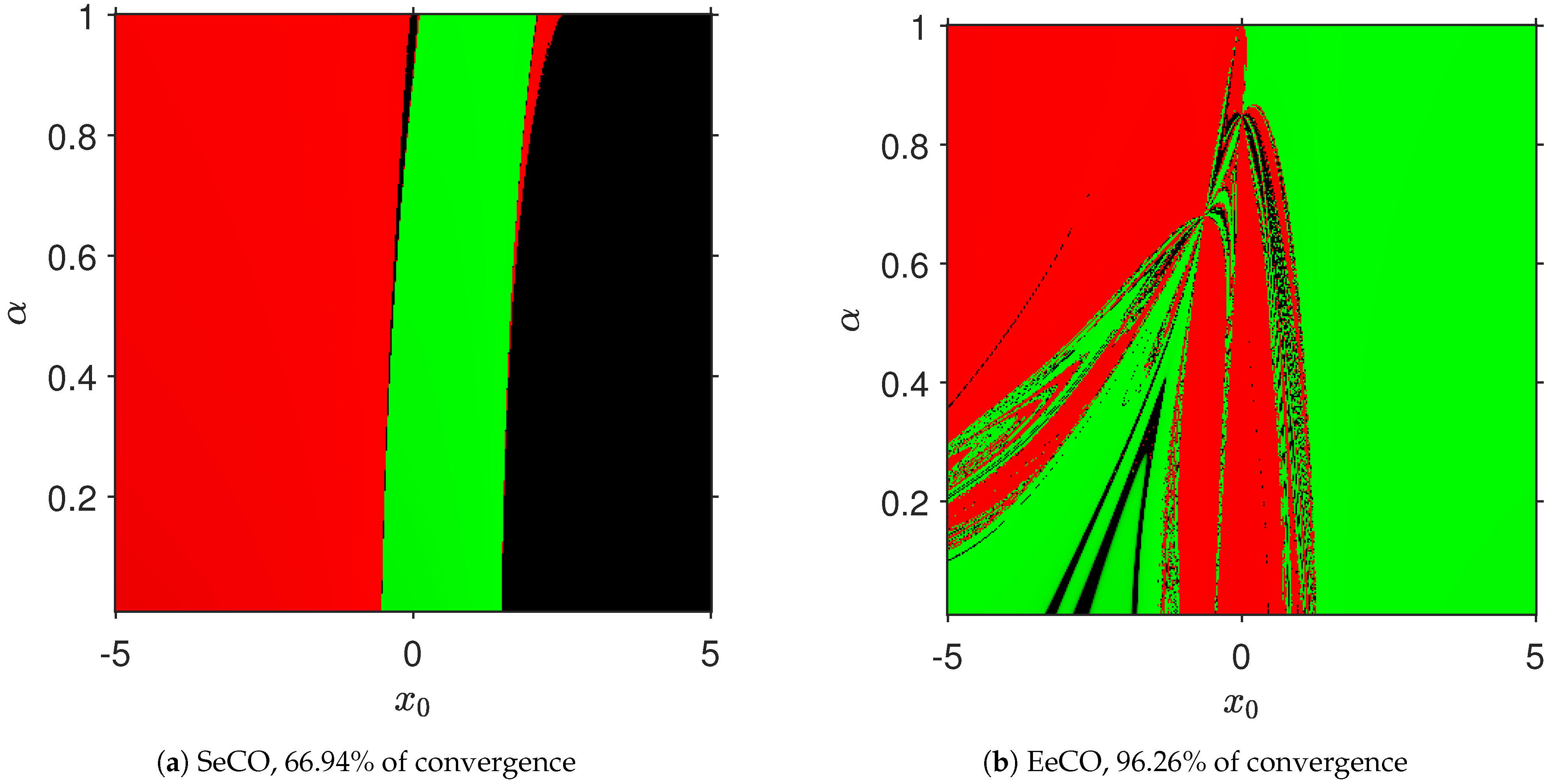
The first test function is $f_1\left(x\right)=-12.84x^6-25.6x^5+16.55x^4-2.21x^3+26.71x^2-4.29x-15.21$, with real and complex roots ${\overline{x}}_1\approx 0.82366+0.24769i$, ${\overline{x}}_2\approx 0.82366-0.24769i$, ${\overline{x}}_3\approx -2.62297$, ${\overline{x}}_4\approx -0.584$, ${\overline{x}}_5\approx -0.21705+0.99911i$, and ${\overline{x}}_6\approx -0.21705-0.99911i$.

In

Table 1. Results for $f_1\left(x\right)$, with initial estimates $x_0=-0.58$ for SeCO, and $x_{-1}=0.42$ and $x_0=-0.58$ for EeCO.

	SeCO Method					EeCO Method
$\mathit{\alpha }$	$\overline{\mathit{x}}$	${\mathit{f}}_{\mathit{1}}\left({\mathit{x}}_{\mathit{k}+\mathit{1}}\right)$	${\mathit{x}}_{\mathit{k}+\mathit{1}}-{\mathit{x}}_{\mathit{k}}$	Iter	$\mathit{\rho }$	$\overline{\mathit{x}}$	${\mathit{f}}_{\mathit{1}}\left({\mathit{x}}_{\mathit{k}+\mathit{1}}\right)$	${\mathit{x}}_{\mathit{k}+\mathit{1}}-{\mathit{x}}_{\mathit{k}}$	Iter	$\mathit{\rho }$
1	${\overline{x}}_4$	$1.07\times {10}^{-14}$	$2.18\times {10}^{-10}$	5	2.00	${\overline{x}}_4$	$9.95\times {10}^{-14}$	$3.48\times {10}^{-10}$	5	2.38
0.9	${\overline{x}}_4$	$2.06\times {10}^{-13}$	$4.04\times {10}^{-9}$	5	2.01	${\overline{x}}_4$	$3.60\times {10}^{-10}$	$6.53\times {10}^{-8}$	5	2.47
0.8	${\overline{x}}_4$	$3.48\times {10}^{-11}$	$6.31\times {10}^{-8}$	5	2.03	${\overline{x}}_4$	$1.50\times {10}^{-10}$	$3.71\times {10}^{-8}$	5	2.23
0.7	${\overline{x}}_4$	$6.78\times {10}^{-9}$	$7.87\times {10}^{-7}$	5	2.07	${\overline{x}}_4$	$6.02\times {10}^{-12}$	$6.64\times {10}^{-9}$	4	1.48
0.6	${\overline{x}}_4$	$2.04\times {10}^{-12}$	$1.22\times {10}^{-8}$	6	2.02	${\overline{x}}_4$	$1.88\times {10}^{-9}$	$3.22\times {10}^{-7}$	4	0.90
0.5	${\overline{x}}_4$	$6.98\times {10}^{-9}$	$6.37\times {10}^{-7}$	6	2.07	${\overline{x}}_4$	$3.39\times {10}^{-9}$	$4.64\times {10}^{-7}$	4	0.80
0.4	${\overline{x}}_4$	$9.73\times {10}^{-11}$	$6.72\times {10}^{-8}$	7	2.04	${\overline{x}}_4$	$5.25\times {10}^{-9}$	$5.85\times {10}^{-7}$	4	0.74
0.3	${\overline{x}}_4$	$5.16\times {10}^{-12}$	$1.39\times {10}^{-8}$	8	2.02	${\overline{x}}_4$	$8.13\times {10}^{-9}$	$7.30\times {10}^{-7}$	4	0.70
0.2	${\overline{x}}_4$	$6.36\times {10}^{-13}$	$4.01\times {10}^{-9}$	9	2.02	${\overline{x}}_4$	$2.24\times {10}^{-13}$	$2.09\times {10}^{-10}$	5	2.53
0.1	${\overline{x}}_4$	$2.16\times {10}^{-11}$	$2.24\times {10}^{-8}$	9	2.03	${\overline{x}}_4$	$6.54\times {10}^{-13}$	$3.29\times {10}^{-10}$	5	2.63

, we can see that SeCO can require the same number of iterations as the classical Steffensen’s method (when $\alpha =1$), and $\rho$ can be slightly higher than 2 when $\alpha \ne 1$. Note that SeCO needs the initial estimate $x_0$ to be very close to ${\overline{x}}_4$ to converge with any $\alpha$. We observe that EeCO require in some cases less iterations than Secant scheme for most values of $\alpha$, and the ACOC can be slightly higher than 1.618.

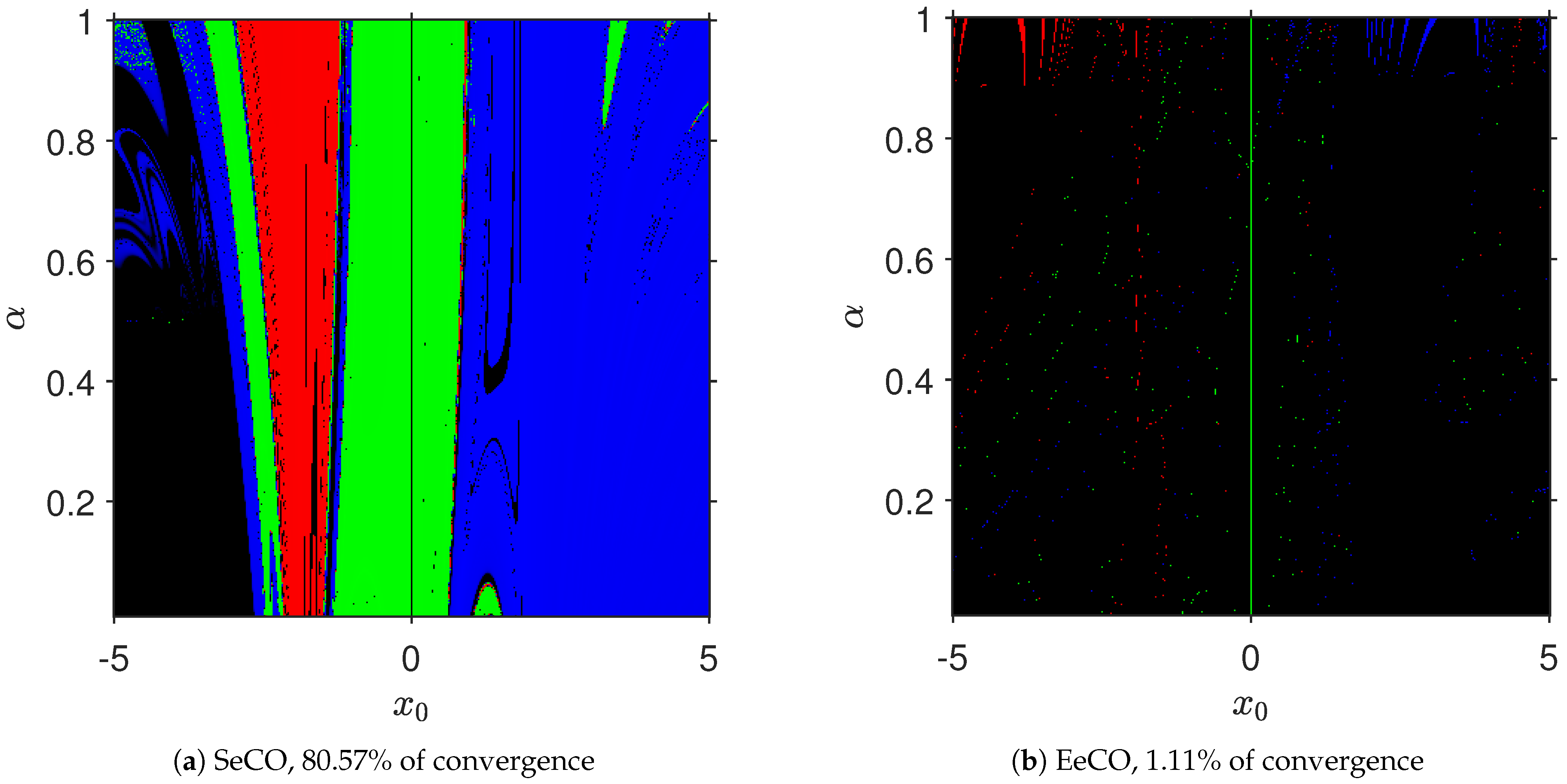
Our second test function is $f_2\left(x\right)=sinx-x^2+1$, with real roots ${\overline{x}}_1\approx -0.6367$ and ${\overline{x}}_2\approx 1.4096$.

In

Table 2. Results for $f_2\left(x\right)$, with initial estimates $x_0=2$ for SeCO, and $x_{-1}=3$ and $x_0=2$ for EeCO.

	SeCO Method					EeCO Method
$\mathit{\alpha }$	$\overline{\mathit{x}}$	${\mathit{f}}_{\mathit{2}}\left({\mathit{x}}_{\mathit{k}+\mathit{1}}\right)$	${\mathit{x}}_{\mathit{k}+\mathit{1}}-{\mathit{x}}_{\mathit{k}}$	Iter	$\mathit{\rho }$	$\overline{\mathit{x}}$	${\mathit{f}}_{\mathit{2}}\left({\mathit{x}}_{\mathit{k}+\mathit{1}}\right)$	${\mathit{x}}_{\mathit{k}+\mathit{1}}-{\mathit{x}}_{\mathit{k}}$	Iter	$\mathit{\rho }$
1	${\overline{x}}_2$	$6.30\times {10}^{-12}$	$1.60\times {10}^{-6}$	6	2.01	${\overline{x}}_2$	$1.26\times {10}^{-10}$	$5.21\times {10}^{-7}$	6	1.62
0.9	${\overline{x}}_1$	$2.93\times {10}^{-14}$	$1.20\times {10}^{-7}$	5	2.00	${\overline{x}}_2$	$1.59\times {10}^{-9}$	$2.28\times {10}^{-6}$	6	1.62
0.8	-	-	-	-	-	${\overline{x}}_2$	$1.47\times {10}^{-13}$	$6.57\times {10}^{-7}$	7	1.63
0.7	-	-	-	>500	-	${\overline{x}}_2$	$6.32\times {10}^{-12}$	$6.13\times {10}^{-8}$	7	1.63
0.6	-	-	-	>500	-	${\overline{x}}_2$	$2.04\times {10}^{-10}$	$4.78\times {10}^{-7}$	7	1.64
0.5	-	-	-	>500	-	${\overline{x}}_2$	$4.93\times {10}^{-9}$	$3.11\times {10}^{-6}$	7	1.65
0.4	-	-	-	>500	-	${\overline{x}}_2$	$3.84\times {10}^{-12}$	$3.46\times {10}^{-8}$	8	1.61
0.3	-	-	-	>500	-	${\overline{x}}_2$	$3.46\times {10}^{-10}$	$5.10\times {10}^{-7}$	8	1.60
0.2	-	-	-	>500	-	${\overline{x}}_2$	$3.97\times {10}^{-13}$	$6.88\times {10}^{-9}$	9	1.64
0.1	-	-	-	>500	-	${\overline{x}}_2$	$9.16\times {10}^{-11}$	$1.82\times {10}^{-7}$	9	1.65

we note that SeCO can converge in fewer iterations than its classical partner, and a different root can be found; case $\alpha =0.8$ is not shown because this method converges to some point which is not a root of $f_2\left(x\right)$, due to one of the stopping criteria is much greater than zero, also, no results are shown when it is required more than 500 iterations. We can see that EeCO can require the same number of iterations of its classical partner, and $\rho$ can be slightly higher than 1.618.

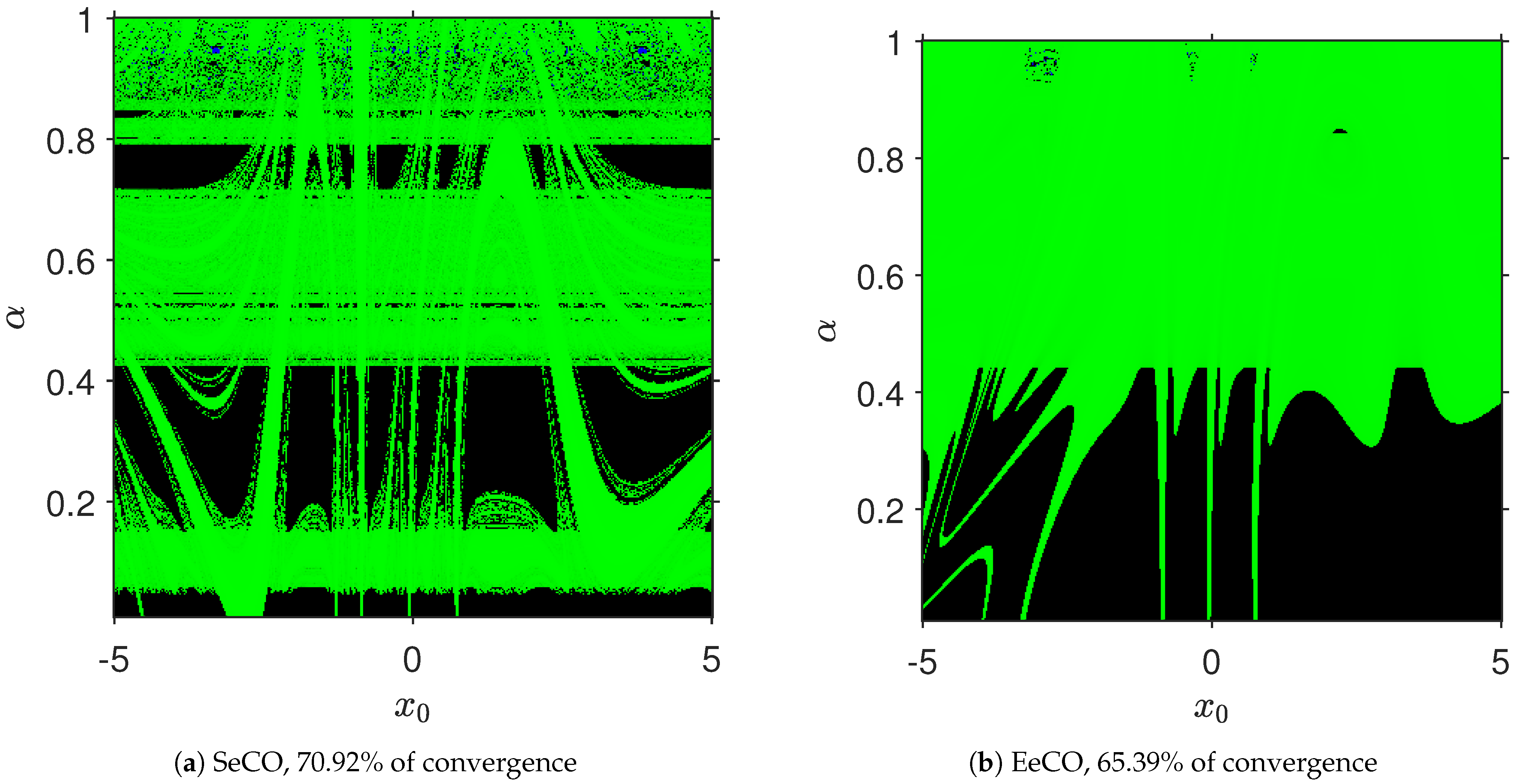
Next test function is $f_3\left(x\right)={\left(sinx-\frac{x}{2}\right)}^2$, with double roots ${\overline{x}}_1\approx -1.8956$, ${\overline{x}}_2=0$, and ${\overline{x}}_3\approx 1.8956$.

In

Table 3. Results for $f_3\left(x\right)$, with initial estimates $x_0=1$ for SeCO, and $x_{-1}=2$ and $x_0=1$ for EeCO.

	SeCO Method					EeCO Method
$\mathit{\alpha }$	$\overline{\mathit{x}}$	${\mathit{f}}_{\mathit{3}}\left({\mathit{x}}_{\mathit{k}+\mathit{1}}\right)$	${\mathit{x}}_{\mathit{k}+\mathit{1}}-{\mathit{x}}_{\mathit{k}}$	Iter	$\mathit{\rho }$	$\overline{\mathit{x}}$	${\mathit{f}}_{\mathit{3}}\left({\mathit{x}}_{\mathit{k}+\mathit{1}}\right)$	${\mathit{x}}_{\mathit{k}+\mathit{1}}-{\mathit{x}}_{\mathit{k}}$	Iter	$\mathit{\rho }$
1	${\overline{x}}_3$	$7.62\times {10}^{-9}$	$1.07\times {10}^{-4}$	18	1.00	${\overline{x}}_3$	$5.84\times {10}^{-9}$	$5.77\times {10}^{-5}$	19	1.00
0.9	${\overline{x}}_3$	$4.88\times {10}^{-9}$	$8.53\times {10}^{-5}$	20	1.00	${\overline{x}}_3$	$4.65\times {10}^{-9}$	$4.79\times {10}^{-5}$	24	1.00
0.8	${\overline{x}}_3$	$3.27\times {10}^{-9}$	$6.98\times {10}^{-5}$	19	1.00	-	-	-	-	-
0.7	${\overline{x}}_3$	$6.76\times {10}^{-9}$	$1.00\times {10}^{-4}$	19	1.00	${\overline{x}}_2$	$8.88\times {10}^{-9}$	$9.43\times {10}^{-5}$	23	1.00
0.6	${\overline{x}}_3$	$3.17\times {10}^{-9}$	$6.88\times {10}^{-5}$	12	1.00	${\overline{x}}_2$	$6.28\times {10}^{-9}$	$7.33\times {10}^{-5}$	26	1.00
0.5	${\overline{x}}_3$	$3.03\times {10}^{-9}$	$6.72\times {10}^{-5}$	18	1.00	${\overline{x}}_3$	$7.23\times {10}^{-9}$	$4.28\times {10}^{-5}$	53	1.00
0.4	${\overline{x}}_3$	$3.37\times {10}^{-9}$	$7.08\times {10}^{-5}$	14	1.00	-	-	-	-	-
0.3	${\overline{x}}_3$	$4.45\times {10}^{-9}$	$8.14\times {10}^{-5}$	9	1.00	${\overline{x}}_3$	$6.04\times {10}^{-9}$	$3.24\times {10}^{-5}$	57	1.00
0.2	${\overline{x}}_3$	$7.05\times {10}^{-9}$	$1.03\times {10}^{-6}$	9	1.00	${\overline{x}}_3$	$9.30\times {10}^{-9}$	$3.64\times {10}^{-5}$	29	1.00
0.1	${\overline{x}}_3$	$7.57\times {10}^{-9}$	$1.06\times {10}^{-4}$	16	1.00	${\overline{x}}_3$	$9.72\times {10}^{-9}$	$3.35\times {10}^{-5}$	55	1.01

, we observe that many times SeCO requires lower number of iterations than Steffensen’s procedure, and the ACOC is linear for all $\alpha$, because the multiplicity of all roots is $m=2$. We note that number of iterations is increasing when EeCO is used, a distinct root can be found when a different value of $\alpha$ is chosen, and again, $\rho$ is linear for any $\alpha$, because the multiplicity of these roots is 2; we show no results for $\alpha =0.8,0.4$ as this scheme converges to some point which is not a root of $f_3\left(x\right)$, due to one of the stopping criteria is much greater than zero.

The fourth nonlinear function is $f_4\left(x\right)=\sqrt{x^4+8}sin\left(\frac{\pi }{x^2+2}\right)+\frac{x^3}{x^4+1}-\sqrt{6}+\frac{8}{17}$, with roots ${\overline{x}}_1=-2$ and ${\overline{x}}_2\approx -1.1492$.

In

Table 4. Results for $f_4\left(x\right)$, with initial estimates $x_0=-3$ for SeCO, and $x_{-1}=-2$ and $x_0=-3$ for EeCO.

	SeCO Method					EeCO Method
$\mathit{\alpha }$	$\overline{\mathit{x}}$	${\mathit{f}}_{\mathit{4}}\left({\mathit{x}}_{\mathit{k}+\mathit{1}}\right)$	${\mathit{x}}_{\mathit{k}+\mathit{1}}-{\mathit{x}}_{\mathit{k}}$	Iter	$\mathit{\rho }$	$\overline{\mathit{x}}$	${\mathit{f}}_{\mathit{4}}\left({\mathit{x}}_{\mathit{k}+\mathit{1}}\right)$	${\mathit{x}}_{\mathit{k}+\mathit{1}}-{\mathit{x}}_{\mathit{k}}$	Iter	$\mathit{\rho }$
1	${\overline{x}}_1$	$1.37\times {10}^{-14}$	$4.18\times {10}^{-7}$	4	2.04	-	-	-	-	-
0.9	${\overline{x}}_1$	$1.67\times {10}^{-15}$	$1.67\times {10}^{-7}$	4	2.04	${\overline{x}}_1$	$4.88\times {10}^{-9}$	$2.41\times {10}^{-5}$	4	1.18
0.8	${\overline{x}}_1$	$1.00\times {10}^{-16}$	$4.57\times {10}^{-8}$	4	2.03	${\overline{x}}_1$	$1.21\times {10}^{-9}$	$5.24\times {10}^{-6}$	5	2.75
0.7	${\overline{x}}_1$	$2.47\times {10}^{-9}$	$2.35\times {10}^{-4}$	3	1.56	${\overline{x}}_1$	$2.53\times {10}^{-9}$	$1.14\times {10}^{-5}$	9	1.49
0.6	${\overline{x}}_1$	$1.75\times {10}^{-10}$	$8.66\times {10}^{-5}$	3	1.72	-	-	-	-	-
0.5	${\overline{x}}_1$	$7.05\times {10}^{-9}$	0.0335	2	-	-	-	-	-	-
0.4	${\overline{x}}_1$	$3.04\times {10}^{-9}$	$3.02\times {10}^{-4}$	3	1.78	-	-	-	-	-
0.3	${\overline{x}}_1$	$9.20\times {10}^{-13}$	$3.60\times {10}^{-6}$	4	2.01	-	-	-	-	-
0.2	${\overline{x}}_1$	$6.99\times {10}^{-15}$	$2.40\times {10}^{-7}$	5	2.00	-	-	-	-	-
0.1	-	-	-	-	-	-	-	-	-	-

, we see that SeCO needs fewer iterations than its classical partner in many cases; $\rho$ is not provided for $\alpha =0.5$ because it is necessary at least three iterations to be computed, and we do not show results for $\alpha =0.1$ as this procedure does not converge to a root of $f_4\left(x\right)$. We can observe that the classical Secant method has failed, whereas, the conformable version can find solution for some values of $\alpha$, and the ACOC can be slightly higher than 1.618; and again, no results are shown for $\alpha =0.1,0.2,0.3,0.4,0.5,0.6$ because this procedure does not converge to a root of $f_4\left(x\right)$.

The fifth test function is $f_5\left(x\right)=\sqrt{x^4+8}sin\left(\frac{\pi }{x^2+2}+\frac{x^3}{x^4+1}\right)-\sqrt{6}+\frac{8}{17}$, with real root ${\overline{x}}_1\approx -0.8541$. Also, the complex root ${\overline{x}}_2\approx -0.1498+0.8244i$ can be obtained.

In

Table 5. Results for $f_5\left(x\right)$, with initial estimates $x_0=-3$ for SeCO, and $x_{-1}=-2$ and $x_0=-3$ for EeCO.

	SeCO Method					EeCO Method
$\mathit{\alpha }$	$\overline{\mathit{x}}$	${\mathit{f}}_{\mathit{5}}\left({\mathit{x}}_{\mathit{k}+\mathit{1}}\right)$	${\mathit{x}}_{\mathit{k}+\mathit{1}}-{\mathit{x}}_{\mathit{k}}$	Iter	$\mathit{\rho }$	$\overline{\mathit{x}}$	${\mathit{f}}_{\mathit{5}}\left({\mathit{x}}_{\mathit{k}+\mathit{1}}\right)$	${\mathit{x}}_{\mathit{k}+\mathit{1}}-{\mathit{x}}_{\mathit{k}}$	Iter	$\mathit{\rho }$
1	${\overline{x}}_1$	$3.84\times {10}^{-10}$	$1.37\times {10}^{-5}$	11	2.09	${\overline{x}}_1$	$8.84\times {10}^{-13}$	$2.31\times {10}^{-8}$	11	2.51
0.9	${\overline{x}}_2$	$7.17\times {10}^{-12}$	$2.86\times {10}^{-7}$	131	2.00	${\overline{x}}_1$	$2.03\times {10}^{-9}$	$4.21\times {10}^{-6}$	9	1.06
0.8	${\overline{x}}_1$	$1.40\times {10}^{-9}$	$2.22\times {10}^{-5}$	15	3.01	${\overline{x}}_1$	$1.31\times {10}^{-12}$	$4.45\times {10}^{-8}$	11	1.36
0.7	${\overline{x}}_1$	$3.05\times {10}^{-10}$	$9.44\times {10}^{-6}$	33	2.67	${\overline{x}}_1$	$2.99\times {10}^{-14}$	$3.67\times {10}^{-9}$	8	1.49
0.6	${\overline{x}}_1$	$1.46\times {10}^{-12}$	$5.94\times {10}^{-7}$	17	1.97	${\overline{x}}_1$	$9.44\times {10}^{-11}$	$3.79\times {10}^{-7}$	7	1.89
0.5	${\overline{x}}_1$	$4.63\times {10}^{-11}$	$3.03\times {10}^{-6}$	7	2.04	${\overline{x}}_1$	$2.73\times {10}^{-9}$	$1.89\times {10}^{-6}$	6	3.60
0.4	${\overline{x}}_1$	$1.22\times {10}^{-15}$	$5.75\times {10}^{-9}$	9	1.76	-	-	-	>500	-
0.3	-	-	-	>500	-	-	-	-	>500	-
0.2	-	-	-	>500	-	-	-	-	>500	-
0.1	${\overline{x}}_1$	$4.59\times {10}^{-11}$	$2.00\times {10}^{-6}$	7	2.04	-	-	-	>500	-

, we note that SeCO can require fewer iterations than its classical version in some cases, a different root can be found when choosing a distinct value of $\alpha$, a complex root can be obtained starting from a real initial estimate, and $\rho$ can be slightly higher than 2. We can see that EeCO can converge in a lower number of iterations than its classical version, and the ACOC can be slightly higher than 1.618. No results are shown in both methods when they require more than 500 iterations.

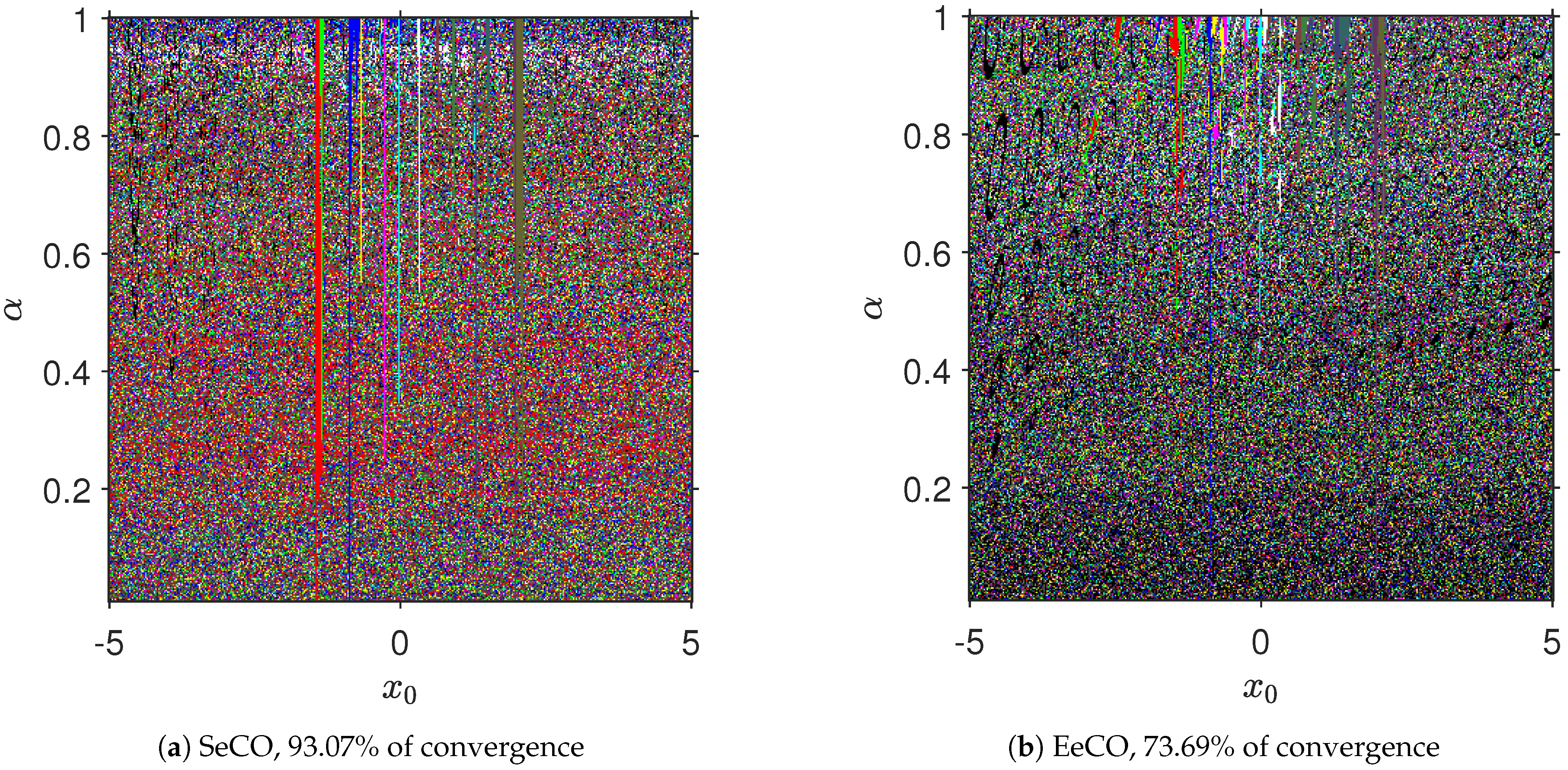
Finally, our sixth test function is $f_6\left(x\right)=sin10x-0.5x+0.2$, with real roots ${\overline{x}}_1=-1.4523$, ${\overline{x}}_2=-1.3647$, ${\overline{x}}_3=-0.87345$, ${\overline{x}}_4=-0.6857$, ${\overline{x}}_5=-0.27949$, ${\overline{x}}_6=-0.021219$, ${\overline{x}}_7=0.31824$, ${\overline{x}}_8=0.64036$, ${\overline{x}}_9=0.91636$, ${\overline{x}}_{10}=1.3035$, ${\overline{x}}_{11}=1.5118$, ${\overline{x}}_{12}=1.9756$, and ${\overline{x}}_{13}=2.0977$.

In

Table 6. Results for $f_6\left(x\right)$, with initial estimates $x_0=3$ for SeCO, and $x_{-1}=4$ and $x_0=3$ for EeCO.

	SeCO Method					EeCO Method
$\mathit{\alpha }$	$\overline{\mathit{x}}$	${\mathit{f}}_{\mathit{6}}\left({\mathit{x}}_{\mathit{k}+\mathit{1}}\right)$	${\mathit{x}}_{\mathit{k}+\mathit{1}}-{\mathit{x}}_{\mathit{k}}$	Iter	$\mathit{\rho }$	$\overline{\mathit{x}}$	${\mathit{f}}_{\mathit{6}}\left({\mathit{x}}_{\mathit{k}+\mathit{1}}\right)$	${\mathit{x}}_{\mathit{k}+\mathit{1}}-{\mathit{x}}_{\mathit{k}}$	Iter	$\mathit{\rho }$
1	${\overline{x}}_3$	$6.38\times {10}^{-15}$	$5.41\times {10}^{-9}$	20	2.00	${\overline{x}}_{10}$	$4.48\times {10}^{-12}$	$2.41\times {10}^{-8}$	17	1.20
0.9	${\overline{x}}_{13}$	$1.57\times {10}^{-12}$	$7.60\times {10}^{-8}$	16	2.01	${\overline{x}}_7$	$1.46\times {10}^{-10}$	$9.06\times {10}^{-7}$	10	0.74
0.8	${\overline{x}}_4$	$1.85\times {10}^{-12}$	$7.12\times {10}^{-8}$	18	1.99	${\overline{x}}_2$	$1.60\times {10}^{-11}$	$3.61\times {10}^{-8}$	11	1.31
0.7	${\overline{x}}_1$	$6.41\times {10}^{-12}$	$1.39\times {10}^{-7}$	28	2.02	${\overline{x}}_9$	$6.89\times {10}^{-10}$	$4.16\times {10}^{-7}$	24	1.38
0.6	${\overline{x}}_1$	$6.33\times {10}^{-13}$	$3.88\times {10}^{-8}$	23	2.01	${\overline{x}}_9$	$6.14\times {10}^{-11}$	$1.03\times {10}^{-7}$	23	1.14
0.5	${\overline{x}}_{11}$	$1.09\times {10}^{-9}$	$1.17\times {10}^{-6}$	21	1.95	${\overline{x}}_{10}$	$2.32\times {10}^{-12}$	$6.76\times {10}^{-9}$	20	1.81
0.4	${\overline{x}}_1$	$8.15\times {10}^{-9}$	$3.49\times {10}^{-6}$	95	2.05	${\overline{x}}_5$	$4.45\times {10}^{-13}$	$2.23\times {10}^{-9}$	14	1.98
0.3	-	-	-	-	-	${\overline{x}}_4$	$8.39\times {10}^{-13}$	$3.87\times {10}^{-9}$	104	1.37
0.2	${\overline{x}}_5$	$7.17\times {10}^{-12}$	$8.35\times {10}^{-8}$	66	1.47	${\overline{x}}_{13}$	$2.58\times {10}^{-10}$	$8.57\times {10}^{-8}$	175	1.67
0.1	${\overline{x}}_3$	$7.92\times {10}^{-14}$	$4.44\times {10}^{-9}$	58	2.00	-	-	-	>500	-

, we observe that SeCO and EeCO need lower number of iterations than their classical partners, respectively, for some values of $\alpha$, and that $\rho$ is similar to the classical one in each case; no results is shown for $\alpha =0.3$ because this scheme converges to some point which is not a root of $f_6\left(x\right)$, due to one of the stopping criteria is much greater than zero. Neither are results shown for EeCO when $\alpha =0.1$, since it requires more than 500 iterations to converge. We note that with each procedure different roots are obtained by modifying the value of $\alpha$.

Qualitative Performance

Now, we analyze the dependency regarding the initial estimations of the schemes designed in this manuscript; for this, convergence planes defined in [28] are used. In them, the abscissa axis corresponds to the initial estimate $x_0$ (for both schemes), and the order of the derivative $\alpha$ corresponds to the ordinate axis. We define a mesh of $400\times 400$ points that can be represented in different colors. Those not represented in black correspond to the pairs $(x_0,\alpha )$ converging to one of the roots, with a tolerance of ${10}^{-3}$. Different roots have associated different colors. Therefore, a point represented in black means that the iterative process does not converge to any root in a maximum of 500 iterations.

For all convergence planes we calculate the percentage of convergent $(x_0,\alpha )$, to compare the efficiency of these procedures. For each method we set $a=-10$ in each plane, $x_0\in [-5,5]$, and $\alpha \in (0,1]$. In the case of EeCO we select $x_{-1}=x_0+1$ to perform the first iteration, just as we did in the numerical tests in Section 3.

In Figure 1, we can observe that SeCO achieves approximately only 0.2% of convergence, and only one root is obtained, whereas EeCO reaches approximately 43% of convergence, where all the roots are reached.

In Figure 2, SeCO attains around 67% of convergence, and EeCO attains around 97% of convergence. Both roots are obtained on each plane.

In Figure 3, we see that SeCO achieves about 81% of convergence, but EeCO reaches only about 1% of convergence. The three roots are found.

In Figure 4, we observe that SeCO attains approximately 41% of convergence, whereas EeCO attains approximately 24% of convergence. Both roots are obtained on each plane.

In Figure 5, we note that SeCO achieves around 71% of convergence, and EeCO reaches only around 66% of convergence. Both roots (the real an the complex) are found on each plane for different values of $\alpha$. These results improve those obtained for $f_3\left(x\right)$ and $f_4\left(x\right)$.

In Figure 6, we can see that SeCO attains about 93% of convergence, but EeCO attains about 74% of convergence. Let us remark that each method obtains all the roots and the convergence rates are higher in this case than those obtained on the previous functions.

We point out that $f_2\left(x\right)$, $f_3\left(x\right)$, $f_4\left(x\right)$, $f_5\left(x\right)$, and $f_6\left(x\right)$ have infinite roots, so, a higher percentage of converging $(x_0,\alpha )$ could be obtained in Figure 2, Figure 3, Figure 4, Figure 5 and Figure 6 if we consider some of the complex roots of these functions.

5. Concluding Remarks

In this work, the first derivative-free conformable iterative methods in the literature have been designed (SeCO and EeCO), where SeCO is the first optimal derivative-free conformable method, and EeCO is also the first conformable scheme with memory. The convergence of these procedures was analyzed, and these methods preserve the order of convergence of their classical versions (when $\alpha =1$). This fact provides the proposed schemes with more degrees of freedom, as with the same initial estimation, and changing the values of $\alpha$, we can obtain all the roots of the equations or improve the convergence results, in some sense. In order to check these advantages, the numerical performance of these schemes has been studied. Derivative-free conformable procedures converge when the classical versions fail, roots can be found in fewer iterations, a different solution can be obtained by selecting different values of $\alpha$, complex roots can be achieved with real seeds, and the approximated computational order of convergence can be slightly higher. Also, we visualized the dependence on initial estimates by using convergence planes, and these methods showed good stability, due to the percentage of converging points $(x_0,\alpha )$, furthermore, all roots are obtained in most of planes. Therefore, the set of converging initial estimations is wider in the case of conformable derivative-free methods.