Turbulence Removal in Atmospheric Dynamics through Laminar Channels

Abstract

Dynamics in atmospheric structures are analyzed using the Scale Relativity Theory in Schrödinger-type and Madelung-type scenarios. In the Schrödinger-type scenario, the group invariances of the special linear group SL(2R)-type under Riccati-type gauges implies morphological atmospheric manifestations through frequency modulation, particularly through period doubling. In the Madelung-type scenario, the same group invariances type, manifested through harmonic mappings, implies the functionality of atmospheric mass conductions through mass superconducting-type by scale transition from nondifferentiable atmospheric dynamics to differentiable atmospheric dynamics. The compatibility of these two scenarios under the correlations of atmospheric morphologies-functionalities implies Stoler-type coherences of the atmospheric dynamics through the removal of atmospheric turbulence by means of laminar channels. Finally, these theories are successfully employed to analyze the vertical atmospheric dynamics of cases of insect swarms.

1. Introduction

The usual physical models used in describing the dynamics of the atmosphere are based on the hypothesis of the differentiability of the physical quantities used to describe its evolution. As a consequence, the validity of these models must be understood gradually in areas where differentiability and integrability are still functional [1,2,3,4,5]. However, when discussing nonlinearity and chaoticity in the dynamics of the atmosphere, many differentiable and integrable mathematical procedures are of little use. Therefore, in order to properly describe the atmospheric dynamics, it is necessary to introduce the scale resolution both into the expressions of the physical variables as well as into the expressions of the fundamental equations governing these atmospheric dynamics [6,7,8,9].

Accepting the above affirmation, any physical variable (which might be used in the description of atmospheric dynamics) will depend on both the usual mathematical procedures on spatial and time coordinates as well as on a scale resolution. Specifically, instead of working with a single physical variable (a strictly non-differentiable mathematical function), it is possible to operate only with approximations of this mathematical function, resulting in averaging it at different scale resolutions. Thus, any physical variable used to describe atmospheric dynamics will operate as the limit of a family of mathematical functions, the function being non-differentiable for zero scale resolution and differentiable for non-zero scale resolution [6,7,8,9]. The fractal interpretation is now used in a myriad of scientific applications, most interestingly and recently in the bidirectional associative memory neural networks [10,11,12,13,14].

This new method of describing the dynamics of atmospheric dynamics obviously implies the development of both new geometric structures and physical theories consistent with these geometric structures, for which the laws of motion invariant to time coordinate transformations are also invariant to transformations with respect to scale resolution. Such a geometric structure is one based on the concept of the fractal/multifractal and the corresponding physical model described in the Scale Relativity Theory [7,8,9]. From this perspective, the holographic implementation in the description of the atmospheric dynamics will be made explicit based on the description of the dynamics of the structural units of any atmospheric structures assimilated to atmospheric dynamics by continuous but non-differentiable curves (fractal/multifractal curves). Many recent works exist that consider fluid flows in much more restrained conditions, in most cases relating to improving energy transfer, especially in the context of climate change [15,16]; however, in this case, a study applying to the atmosphere as a whole is considered.

In the present paper, the nonlinear type behaviors are explained in the dynamics of atmospheric systems by using the Scale Relativity Theory model in the form of Schrödinger and Madelung-type scenarios. The holographic character in the description of the atmospheric dynamics will thus be highlighted. Furthermore, what will also be shown is that this interpretation, taken to its conclusion through a Riccati-type gauge, produces nonlinear-type behaviors in the atmospheric multifractal, such as modulation. With this in mind, such theories can be shown to coexist with two theoretical notions developed in our previous papers—first, that “laminar channels” exist in the atmosphere which guides the transport phenomena of the atmosphere, and that the atmosphere can be considered through a mass conductivity theory that furthermore explains such transport. Finally, these theories are tested through telemetric data gathered by two different instruments, more precisely a ceilometer and a radar, with regards to insect swarm vertical dynamics, and it is found that the theory can accurately predict the short-term vertical dynamics of such swarms through the atmosphere.

2. Schrödinger and Madelung-Type Scenarios in the Description of Atmospheric Dynamics

It is a known fact that the dynamics of the atmospheric system in the Scale Relativity Theory [7,8,9] can be described through two instances (scenarios):

(a) The Schrödinger-type scenario, through the multifractal Schrödinger equation:

$${\lambda }^2{\left(dt\right)}^{\left[\frac{4}{f\left(\alpha \right)}\right]-2}{\partial }_l{\partial }^l\mathsf{\Psi }+i\lambda {\left(dt\right)}^{\left[\frac{2}{f\left(\alpha \right)}\right]-1}{\partial }_t\mathsf{\Psi }=0$$

(1)

(b) The Madelung-type scenario, through the multifractal hydrodynamic equations:

$${\partial }_t{V}_D^i+V_D^l{\partial }_l{V}_D^i=-{\partial }^{i}Q$$

(2)

$${\partial }_t\rho +{\partial }_l\left(\rho V_D^l\right)=0$$

(3)

where in Equations (1)–(3) we used the operators:

$${\partial }_t=\frac{\partial }{{\partial }_t}, {\partial }_l=\frac{\partial }{\partial x^l}, {\partial }_l{\partial }^l=\frac{{\partial }^2}{\partial x_l^2}$$

(4)

In the above relations, the meaning of the used quantities is the following:

-

$\Psi$ is the state function of the form:

$$\Psi =\sqrt{\rho }{e}^{is}$$

(5)

where $\sqrt{\rho }$ is the amplitude and $s$ is the phase;

-

$\rho$ is the state density:

$$\rho =\Psi \overline{\Psi }$$

(6)

-

$dt$ is the scale resolution;

-

$x^l$ is the multifractal spatial coordinate;

-

$t$ is the non-multifractal temporal coordinate with the role of an affine parameter of the motion curves (we note that in the Scale Relativity Theory, the dynamics of the entities belonging to any atmospheric system are described through continuous and non-differentiable curves—multifractal curves);

-

$\lambda$ is a parameter associated to the multifractal/non-multifractal scale transition;

-

$f\left(\alpha \right)$ is the singularity spectrum with a singularity index of order $\alpha =\alpha \left(D_F\right)$;

-

$D_F$ is the fractal dimension of the motion curves;

-

$V_D^i$ is the differentiable velocity field:

$$V_D^i=2\lambda {(dt)}^{\left[\frac{2}{f\left(\alpha \right)}\right]-1}{\partial }^{i}s$$

(7)

-

$V_F^i$ is the nondifferentiable velocity field:

$$V_F^i=i\lambda {(dt)}^{\left[\frac{2}{f\left(\alpha \right)}\right]-1}{\partial }^i\ln \rho$$

(8)

-

$Q$ is the multifractal specific potential:

$$Q=-2{\lambda }^2{(dt)}^{\left[\frac{4}{f\left(\alpha \right)}\right]-2}\frac{{\partial }^l{\partial }_l\sqrt{\rho }}{\sqrt{\rho }}=-V_F^i{V}_F^i-\frac{1}{2}\lambda {(dt)}^{\left[\frac{2}{f\left(\alpha \right)}\right]-1}{\partial }_l{V}_F^l$$

(9)

Equation (2) corresponds to the multifractal specific momentum conservation law, while Equation (3) corresponds to the multifractal state density conservation law.

3. Schrödinger-Type Scenarios in the Description of Atmospheric Dynamics

The multifractal Schrödinger equation admits, besides the classical Galilei group proper, an extra set of symmetries that, in general conditions, can be taken in a form involving just one space dimension and time as a special linear group of type SL(2,R) in two variables with three parameters [16,17]. For our current necessities, it is necessary to start with the finite equations of the specific special linear group SL(2,R) and build gradually upon these [18,19] in order to discover the necessary equations. Working in the variables $\left(t,r\right)$, the finite equations of this group are provided by the transformations:

$$t\to \frac{\alpha t+\beta }{\gamma t+\delta }; r\to \frac{r}{\gamma t+\delta }$$

(10)

This transformation is a realization of the special linear group SL(2,R) structure in variables $\left(t,r\right)$, with three essential parameters. Every vector in the tangent space of the special linear group SL(2,R) is a linear combination of three fundamental vectors, the infinitesimal generators:

$$X_1=\frac{\partial }{\partial t}, X_2=t\frac{\partial }{\partial t}+\frac{r}{2}\frac{\partial }{\partial r}, X_3=t^2\frac{\partial }{\partial t}+tr\frac{\partial }{\partial r}$$

(11)

satisfying the basic structure equations:

$$\left[X_1,X_2\right]=X_1, \left[X_2,X_3\right]=X_3, \left[X_3,X_3\right]=-2X_2$$

(12)

which we take as standard commutation relations for this type of algebraic structure throughout the present work.

Now, consider Equation (10), which represents the homographic action of the generic matrix that we denote by $\widehat{M}$:

$$\widehat{M}=\left(\begin{array}{cc}\alpha & \beta \\ \gamma & \delta \end{array}\right)$$

(13)

The problem that we want to solve is the following: to find the relationship between the set of matrices and a set of values of $t$ for which $t$ remains constant. From a geometrical point of view, this means finding the set of points $\left(\alpha ,\beta ,\gamma ,\delta \right)$ that uniquely correspond to the values parameter $t$. Using Equation (10) our problem is solved by a Riccati differential equation which is obtained as a consequence of the constancy of $t:dt=0$:

$$dt+{\omega }_1{t}^2+{\omega }_{2}t+{\omega }_3=0$$

(14)

where we use the following notations:

$${\omega }_1=\frac{\gamma d\alpha -\alpha d\gamma }{\alpha \delta -\beta \gamma }$$

(15a)

$${\omega }_2=\frac{\delta d\alpha -\alpha d\delta +\gamma d\beta -\beta d\gamma }{\alpha \delta -\beta \gamma }$$

(15b)

$${\omega }_3=\frac{\delta d\beta -\beta d\delta }{\alpha \delta -\beta \gamma }$$

(15c)

The three differential forms in Equations (15a)–(15c) constitute what is commonly known as a coframe at any point of absolute space. This coframe allows us to translate the geometric properties of absolute space into algebraic properties related to differential Equation (14).

The simplest of these properties refers to the motion on geodesics of the metric. In this case, the 1-forms ${\omega }_1$, ${\omega }_2$, ${\omega }_3$ are exact differentials in the same parameter, the length of the arc of the geodesic, let us say. Along these geodesics, Equation (14) turns into an ordinary differential equation of the Riccati type:

$$\frac{dt}{ds}=a_1{t}^2+2a_{2}t+a_3$$

(16)

Here, the parameters $a_{1,2,3}$ are constants that characterize a certain geodesic of the family.

For obvious physical reasons, it is therefore important to find the most general solution of Equation (16). In this sense, it is enough to note that the complex numbers:

$$w_0\equiv -\frac{a_2}{a_1}+i\frac{\mathsf{\Omega }}{a_1}, w_0{}^{*}\equiv -\frac{a_2}{a_1}+i\frac{\mathsf{\Omega }}{a_1}, \mathsf{\Omega }\equiv a_3{a}_1-a_2{}^2$$

(17)

which are roots of the quadratic polynomial on the right side of Equation (16), are two solutions of the equation: being constants, their derivative is zero, being roots of the right-hand polynomial, it cancels. So, first, we do the homographic transformation:

$$z=\frac{w-w_0}{w-w_0^{*}}$$

(18)

and now it can be seen through a direct calculation that $\mathrm{z}$ is a solution of the linear and homogeneous equation of the first order:

$$\dot{z}=2i\mathsf{\Omega }z\therefore z\left(t\right)=z\left(0\right)e^{2i\mathsf{\Omega }t}$$

(19)

Therefore, if we conveniently express the initial condition $\mathrm{z}\left(0\right)$, we can provide the general solution of Equation (16) by simply inverting the transformation in Equation (18), with the result:

$$w=\frac{w_0+r{e}^{2i\mathsf{\Omega }\left(t-t_r\right)}{w}_0^{*}}{1+r{e}^{2i\mathsf{\Omega }\left(t-t_r\right)}}$$

(20)

where $r$ and $t_r$ are two real constants that characterize the solution. Using Equation (17), this solution can be written in real terms, i.e.,:

$$z=-\frac{a_2}{a_1}+\frac{\mathsf{\Omega }}{a_1}\left(\frac{2r\sin \left[2\mathsf{\Omega }\left(t-t_r\right)\right]}{1+r^2+2r\cos \left[2\mathsf{\Omega }\left(t-t_r\right)\right]}\left.+i\frac{1-r^2}{1+r^2+2r\cos \left[2\mathsf{\Omega }\left(t-t_r\right)\right]}\right)\right.$$

(21)

which highlights a frequency modulation through Stoler-type coherences [16]. Moreover, if the following notation is performed:

$$r\equiv \coth \tau$$

(22)

Equation (21) becomes:

$$z=R+M\mathsf{\Omega }h$$

(23)

in which $h$ is provided by:

$$h=-i\frac{\cosh \tau -e^{-2i\mathsf{\Omega }\left(t-t_m\right)}\sinh \tau }{\cosh \tau +e^{-2i\mathsf{\Omega }\left(t-t_m\right)}\sinh \tau }$$

(24)

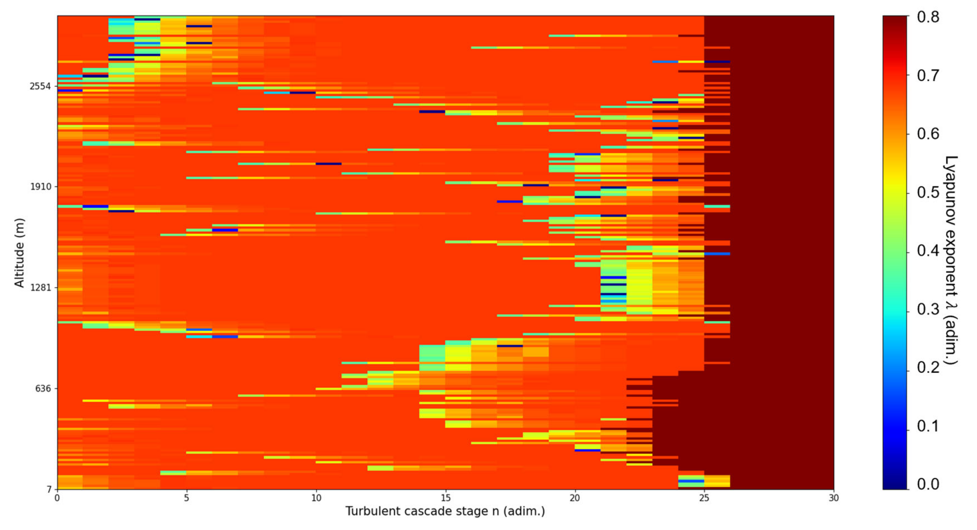
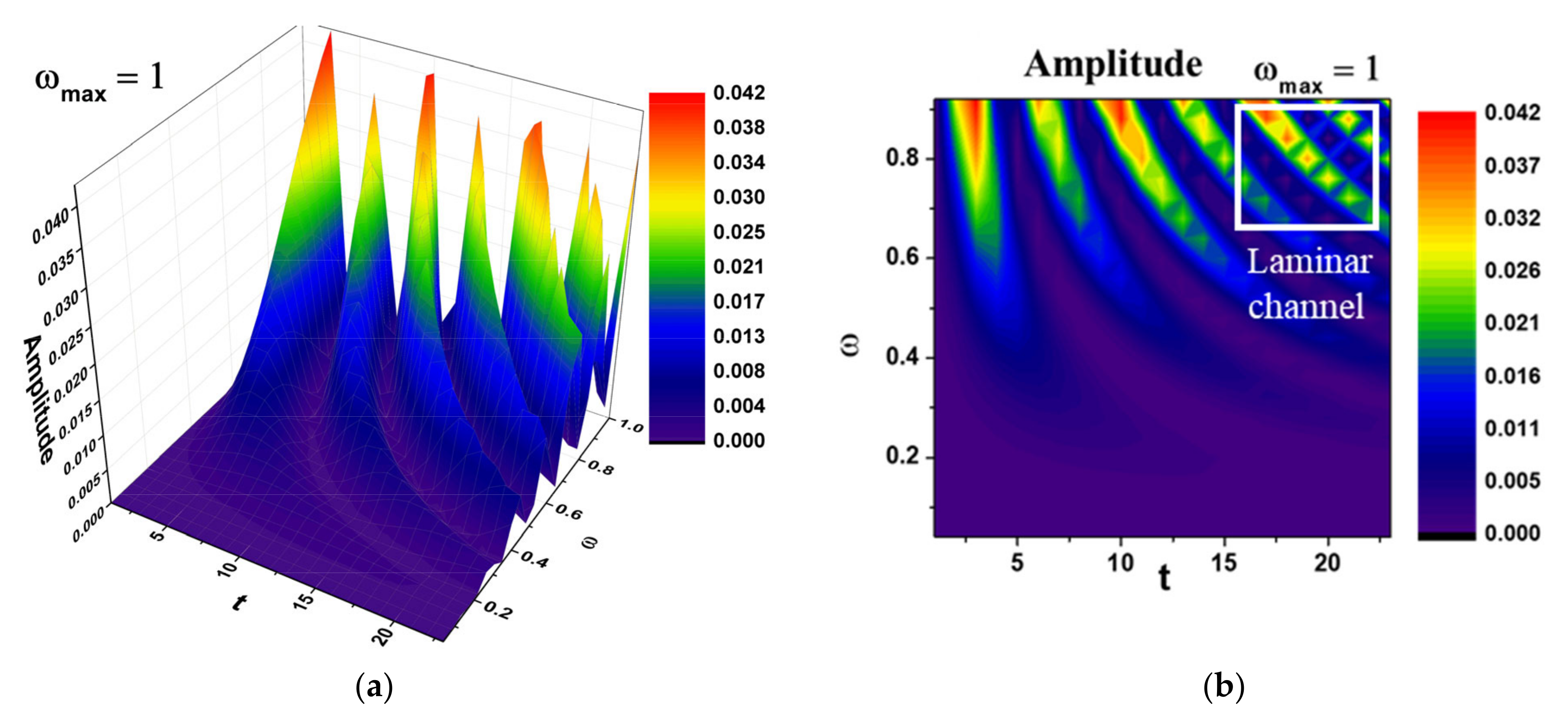
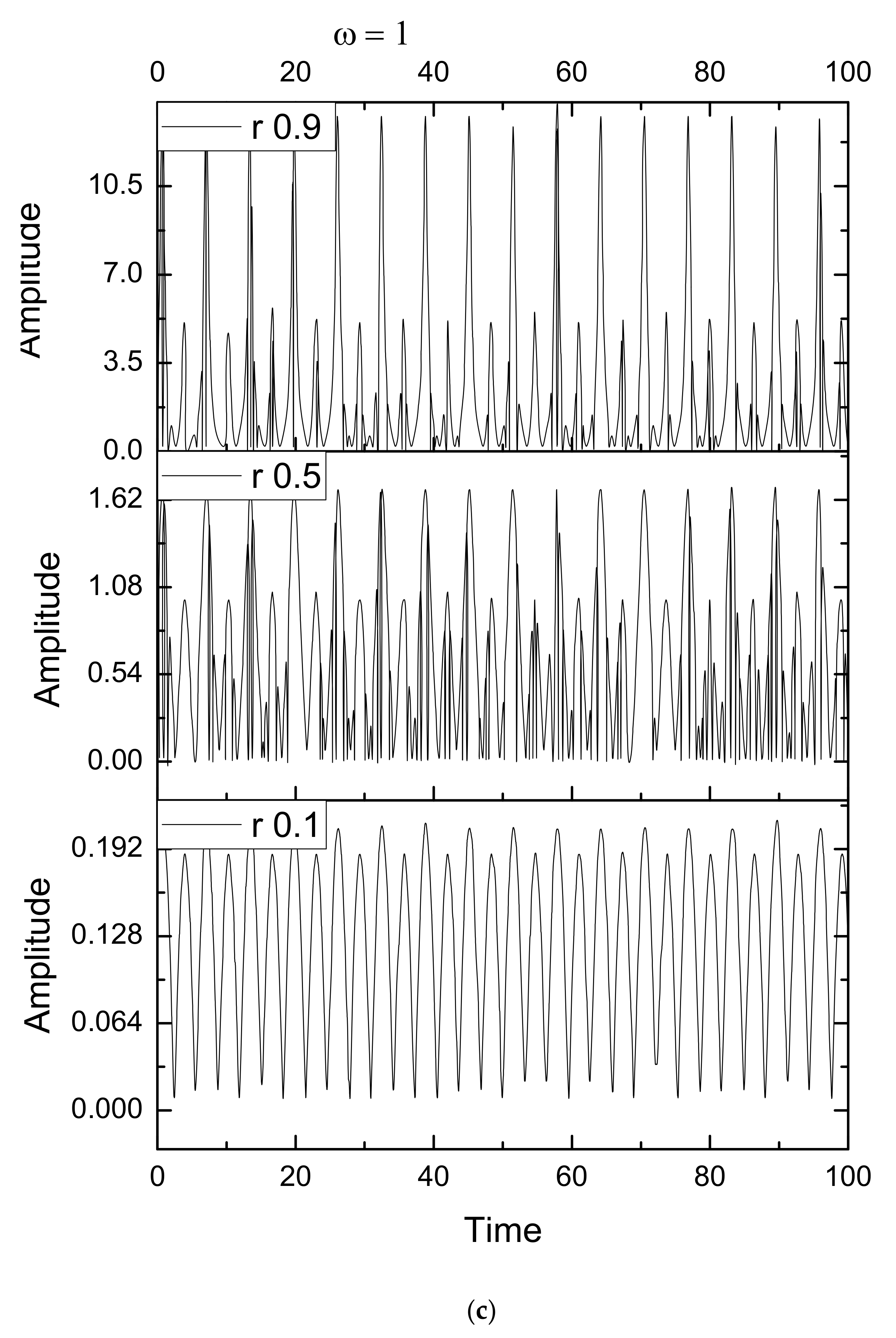
Let us note that Equation (24) can be obtained as a natural result of harmonic mapping from typical Euclidian space to the special linear group SL(2R) [8,9]. We present in Figure 1a–c the dependencies of $Re\left(a_{1}z+a_2\right)$ on the dimensionless coordinates $\mathsf{\Omega }$ and $t$ for various values of $r$. Thus, channel-type morphologies can be mimed through period doubling-type harmonic mappings.

4. Madelung-Type Scenario in the Description of Atmospheric Dynamics

Now, in order to consider and develop the implications of the theory discussed thus far, we refer to our previous works in which the theoretical and practical foundations of what is known as “laminar channels” were made [20,21]. The existence of such channels has already been demonstrated in these studies, but now a different and synergic theoretical justification has been produced for them with the previously demonstrated emergence of nonlinear behaviors in the dynamics of the atmosphere [20,21]. Our previous papers show that a scale transition model can be coupled with a discontinuous form of the Navier-Stokes equation to produce a type of logistic map [21]. Given the occurrence of both chaos and order in this map with the existence of Pomeau-Maneville areas, it was shown that it is possible to identify quasi-laminar or fully laminar regions in atmospheric profiles, leading to “laminar channel” structures that show either ascending or descending behavior [21]. Then, such transitions from laminar to chaotic might come from spontaneous sources, and vice versa, which then suggests that there are laminar channels being modulated throughout the atmosphere—not only that, but the cellular entities found in $Re\left(a_{1}z+a_2\right)$ heavily imply that such laminar areas self-structure in cohesive and coherent ways across space.

The existence of such channels, justified both by previously determined theory and by the newly exposed nonlinear behaviors, also carries numerous implications for mass conduction and energy dissipation in the atmosphere—previously, we assumed the functionality of a conductivity-type relation with regards to atmospheric dynamics using the Madelung scenario [22]. This relation implies the following mass conductivity types:

(a) Mass conductivity at differentiable scale resolutions:

$$\overline{{\sigma }_D}=\sqrt{1+{\theta }^2{\eta }^2}\frac{1+{\theta }^2\xi \eta }{{\theta }^2\left(\xi -\eta \right)}{e}^{\left[-{\mu }^2\frac{{\left(\xi -\eta \right)}^2}{1+{\theta }^2{\eta }^2}\right]}$$

(25)

(b) Mass conductivity at nondifferentiable scale resolutions:

$$\overline{{\sigma }_F}=\sqrt{1+{\theta }^2{\eta }^2}{\left(\frac{\mu }{\theta }\right)}^2{e}^{\left[-{\mu }^2\frac{{\left(\xi -\eta \right)}^2}{1+{\theta }^2{\eta }^2}\right]}$$

(26)

(c) Mass conductivity at global scale resolutions:

$$\overline{\sigma }=\overline{{\sigma }_D}+i\overline{{\sigma }_F}=\sqrt{1+{\theta }^2{\eta }^2}\left[\frac{1+{\theta }^2\xi \eta }{{\theta }^2\left(\xi -\eta \right)}+i{\left(\frac{\mu }{\theta }\right)}^2\right]e^{\left[-{\mu }^2\frac{{\left(\xi -\eta \right)}^2}{1+{\theta }^2{\eta }^2}\right]}$$

(27)

where the following notations were performed:

$$\frac{x}{v_0\tau }=\xi , \frac{t}{\tau }=\eta , \theta =\frac{\lambda {\left(dt\right)}^{\left[\frac{2}{f\left(\alpha \right)}\right]-1}\tau }{a^2}, \mu =\frac{v_0\tau }{a}$$

(28)

In Relations (25)–(27), $\xi$ and $\eta$ are dimensionless coordinates and $a$, $v_0$, and $\tau$ are parameters specific to the mass conduction types. From the Dependencies (25)–(27), it is found that mass conduction in atmospheric dynamics is performed through specific mechanisms dependent on scale resolution and that these mechanisms are reciprocally conditional.

Indeed, if in Equations (25) and (26) we admit that $\theta \to \infty$ (i.e., through (28) with the restriction $f\left(\alpha \right)\to 0$) transitions from nondifferentiable atmospheric dynamics (which are turbulent atmospheric dynamics) to differentiable atmospheric dynamics (which are laminar atmospheric dynamics) are specified in the form:

$$\overline{{\sigma }_D}\to \infty ,\overline{{\sigma }_F}\to 0$$

(29)

Thus, transitions from turbulent atmospheric dynamics to laminar atmospheric dynamics imply infinite mass conduction at differentiable scale resolutions and the absence of mass conduction at nondifferentiable scale resolutions. Furthermore, since for $\theta \to \infty$, the dimensionless force field [17]:

$$\overline{f}={\theta }^2\frac{\xi -\eta }{{\left(1+{\theta }^2{\eta }^2\right)}^2}$$

(30)

also becomes null at all scale resolutions, we can affirm that atmospheric structures with such properties behave in a superconducting manner from the point of view of mass conductivity. The superconducting manner is inferred from the fact that the mass conductivity at differentiable scale resolutions becomes theoretically infinite according to Equation (29), thus implying theoretically perfect mass current and energy transfer through such laminar channels, along with a locally-constant multifractal potential field.

5. Schrödinger and Madelung-Type Scenarios Compatibility in the Description of Atmospheric Dynamics

In the following, we will refer to the compatibility between the two atmospheric dynamics description scenarios based on a special operational procedure: differentiable geometries, variational principles, harmonic mappings, etc. Thus, we shall show that the metric of the Lobachewski plane can be produced as the Cayley metric of a mass conductivity plane for which the following unit circle is found:

$$x^2+y^2=1$$

(31)

where the following notations were performed:

$$x=\frac{{\sigma }_D}{\sqrt{\sigma \overline{\sigma }}}, y=\frac{{\sigma }_F}{\sqrt{\sigma \overline{\sigma }}}$$

(32)

where $\overline{\sigma }$ is the complex conjugate of $\sigma$. In this case, the Lobachewski plane can be placed in a biunivocal correspondence with the interior of the circle. The general metrification procedure of a Cayley space starts from the definition of the metric through the anharmonic ratio as in [19]. We admit that the spatial absolute is provided by the form $\mathsf{\Omega }\left(X,X\right)$, where $X$ is a given vector. Then, the Cayley metric is provided by the differential 2-form:

$$-\frac{d{s}^2}{k^2}=\frac{\mathsf{\Omega }\left(dX,dX\right)}{\mathsf{\Omega }\left(X,X\right)}-\frac{{\mathsf{\Omega }}^2\left(X,dX\right)}{{\mathsf{\Omega }}^2\left(X,X\right)}$$

(33)

where $\mathsf{\Omega }\left(X,Y\right)$ is the duplicate of $\mathsf{\Omega }\left(X,X\right)$, and $k$ is a constant connected to the curvature of the space.

In the case of the Lobachewski plane we shall have:

$$\mathsf{\Omega }\left(X,X\right)=1-x^2-y^2$$

(34a)

$$\mathsf{\Omega }\left(X,dX\right)=-xdx-ydy$$

(34b)

$$\mathsf{\Omega }\left(dX,dX\right)=-d{x}^2-d{y}^2$$

(34c)

from which we obtain:

$$-\frac{d{s}^2}{k^2}=\frac{\left(1-y^2\right)d{x}^2+2xydxdy+\left(1-x^2\right)y^2}{{\left(1-x^2-y^2\right)}^2}$$

(35)

Performing the coordinates transformation:

$$x=\frac{h\overline{h}-1}{h\overline{h}+1}, y=\frac{h+\overline{h}}{h\overline{h}+1}$$

(36)

where $\overline{h}$ is the complex conjugate of $h$, the Metric (35) then becomes:

$$\frac{d{s}^2}{k^2}=-4\frac{dhd\overline{h}}{{\left(h+\overline{h}\right)}^2}$$

(37)

Let us recall that the Relation (37) is invariant of special linear group SL(2R)-type. Continuing, we admit that we can describe the field associated to the mass conductivity through variables $Y^i$ for which we discovered the metric:

$$h_{ij}d{Y}^{i}d{Y}^j$$

(38)

In an ambient space of the metric:

$${\gamma }_{\alpha \beta }d{X}^{\alpha }d{X}^{\beta }$$

(39)

Then, the field equations derive from the variational principle:

$$\delta \int L{\gamma }^{\frac{1}{2}}{d}^{3}x=0$$

(40)

relative to the Lagrange function:

$$L={\gamma }^{\alpha \beta }{h}_{ij}\frac{d{Y}^{i}d{Y}^j}{\partial X^{\alpha }\partial X^{\beta }}$$

(41)

In our case, the Metric (38) is provided through (37), the field variables being $h$ and $\overline{h}$, or equivalently, the real and imaginary part of $h$. In such a frame, we can obtain the following field equations:

$$\left(h-\overline{h}\right){\partial }_l{\partial }^{l}h=2\left({\partial }_{l}h\right)\left({\partial }^{l}h\right)$$

(42a)

$$\left(h-\overline{h}\right){\partial }_l{\partial }^l\overline{h}=2{\partial }_l\overline{h}{\partial }^l\overline{h}$$

(42b)

which admit the following solutions:

$$h=-i\frac{\cosh \mathsf{\Psi }-e^{-i\alpha }\sinh \mathsf{\Psi }}{\cosh \mathsf{\Psi }+e^{-i\alpha }\sinh \mathsf{\Psi }}$$

(43a)

$${\nabla }^2\mathsf{\Psi }=0$$

(43b)

with a real $\alpha$.

In such a context, the similarity between (24) and (43a) specifies the following: (a) the group invariance of the special linear group SL(2R)-type ensures the compatibility between the two scenarios to describe atmospheric dynamics through Stoler-type coherences; (b) the group invariance of the special linear group SL(2R)-type in the Schrödinger-type scenario implies the atmosphere morphologies through frequency modulation; (c) the same group invariance, but in a Madelung-type scenario, implies the atmospheric functionalities through mass conductions. It is then concluded that the previously studied and demonstrated theory of atmospheric mass conductivity is in theoretical accord with the properties of atmospheric laminar channels. Then, it is indeed possible to say that atmospheric transport is greatly simplified in these channels, which, because of the theory presented so far, can be considered as mass superconducting regions of the atmosphere.

With this conclusion, it is possible to imply that, for such regions, atmospheric kinetic energy dissipation is canceled or lessened because of the lack of resistivity—in more familiar terms, this lack of resistivity manifests itself as a decreasing of wind stresses, which are common to laminar flows. Indeed, it has been consistently experimentally shown in our previous studies that stable regions of the atmosphere where conductivity is most decreased, such as the planetary boundary layer, always manifest much lower energy dissipation. Therefore, the theoretical results shown in this paper offer yet another confirmation of the overall theory, and it shall be seen in the following segment that such channels also offer routes of transport for other atmospheric entities.

6. Results

In the following segment, both radar and ceilometer-derived data will be employed to create an experimental application of the theory enumerated thus far. First, an explanation of the main objective of the analysis is warranted. Most current atmospheric studies which employ theoretical and practical means to analyze atmospheric dynamics focus on aerosol transport; however, in this study, insect swarms shall be monitored—the complex relationship between atmospheric insect locomotion and atmospheric parameters is a studied subject [23,24,25]. While in this study the main objective of this experimental analysis is to confirm the theory laid out thus far, the importance of insect swarm monitorization is well known, given the local damage these insects can produce in various agricultural domains [23,24,25]. It is worth noting that, while the laminar channel analysis is performed with ceilometer data, the overall dynamics of the insect swarm is retrieved by radar—thus, a correlation between the two would offer a great confirmation of the theory given the fact that the results of two different platforms would coincide.

In order for our theoretical results to be compared to real data, laminar data must be calculated as per the previously explained methods with ceilometer data, and radar data must be extracted to monitor and compare with laminar data the insect swarm vertical dynamics. The ceilometer platform utilized in this study is a CHM15k ceilometer operating at a 1064 nm wavelength, and the radar platform is a DJUG RPG-FMCW-94-DP Doppler non-scanning cloud radar platform [26]. Both are positioned in Galați, Romania, at the UGAL–REXDAN facility found at coordinates 45.435125N, 28.036792E, 65 m above sea level, which is a part of the “Dunărea de Jos” University of Galați [26]. These instruments have been chosen and set up to conform to the standards imposed by the Aerosol Clouds and Trace Gases Research Infrastructure community [26]. From a computational perspective, the necessary calculations are performed through code written and operated in Python 3.10.

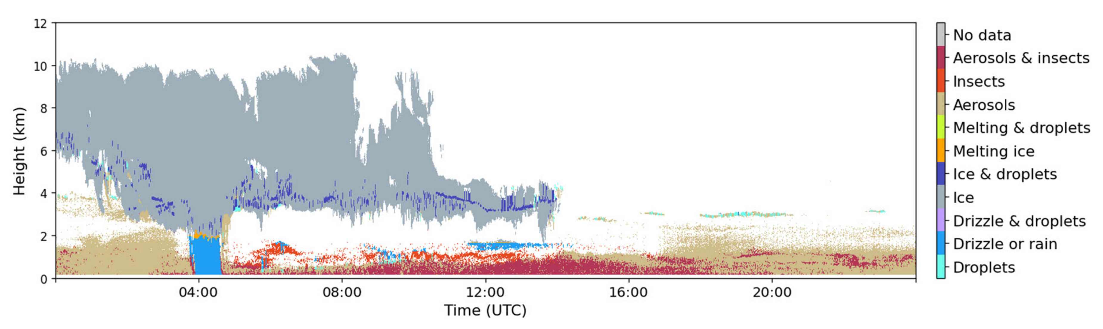
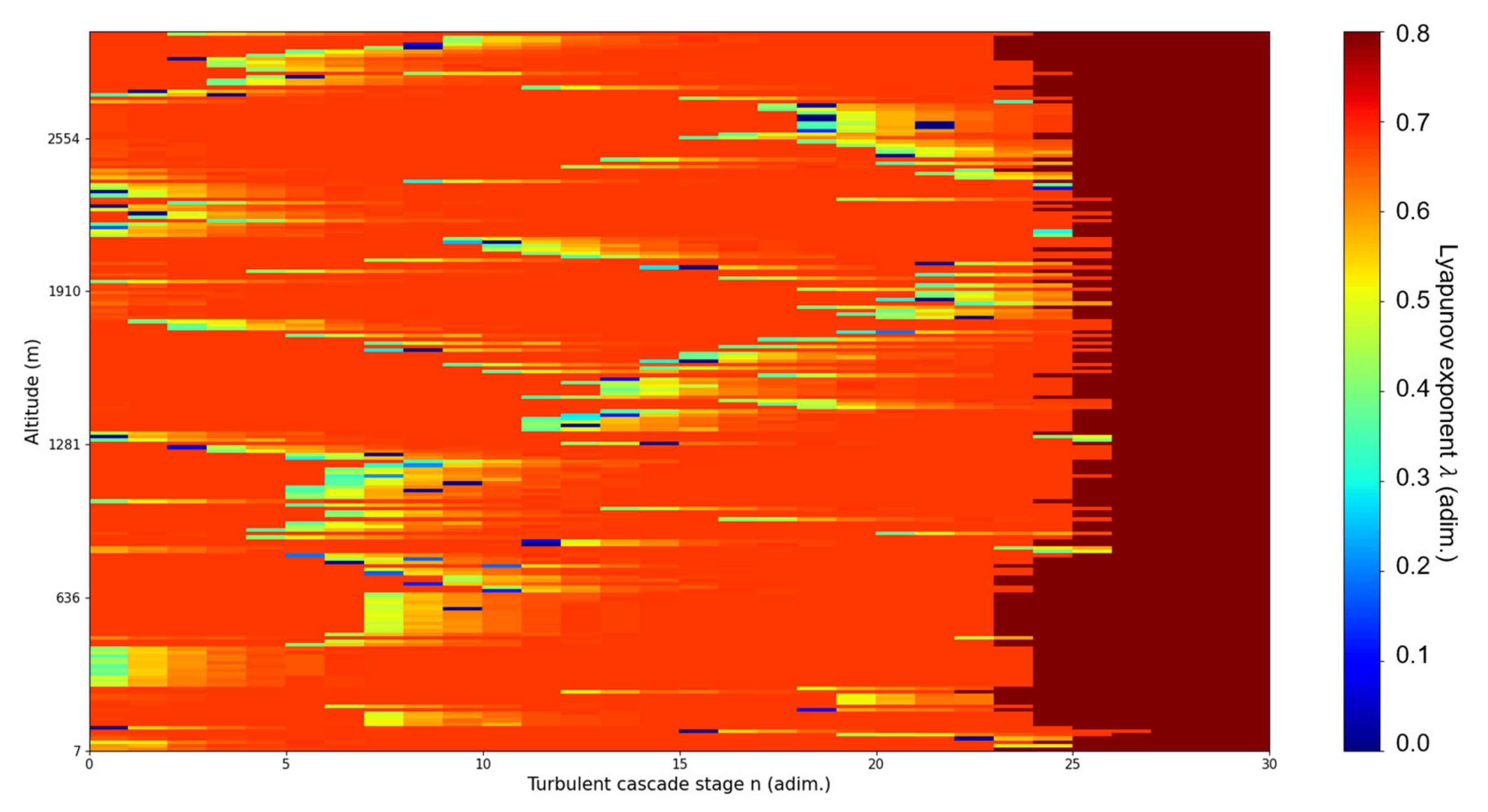
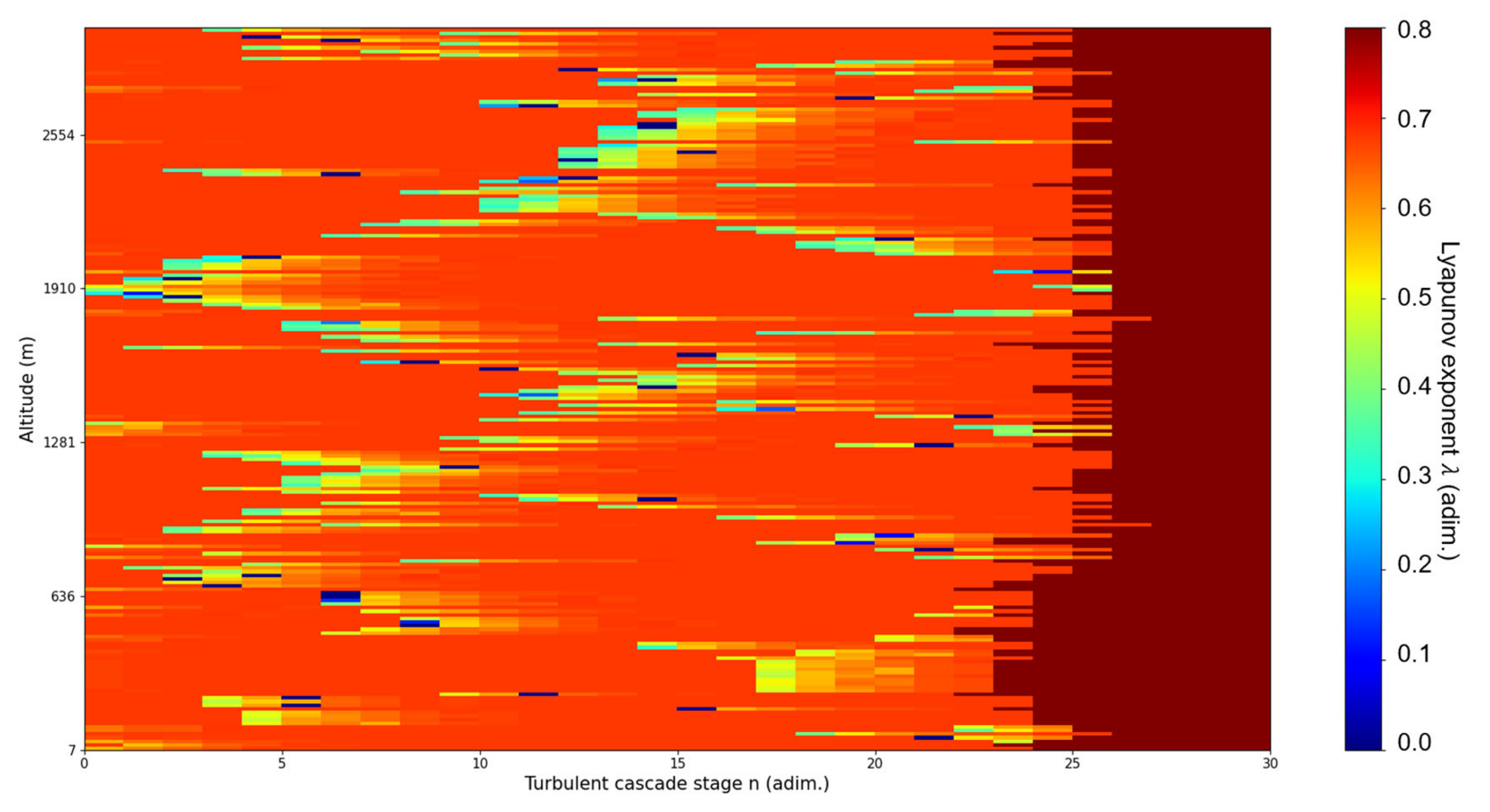
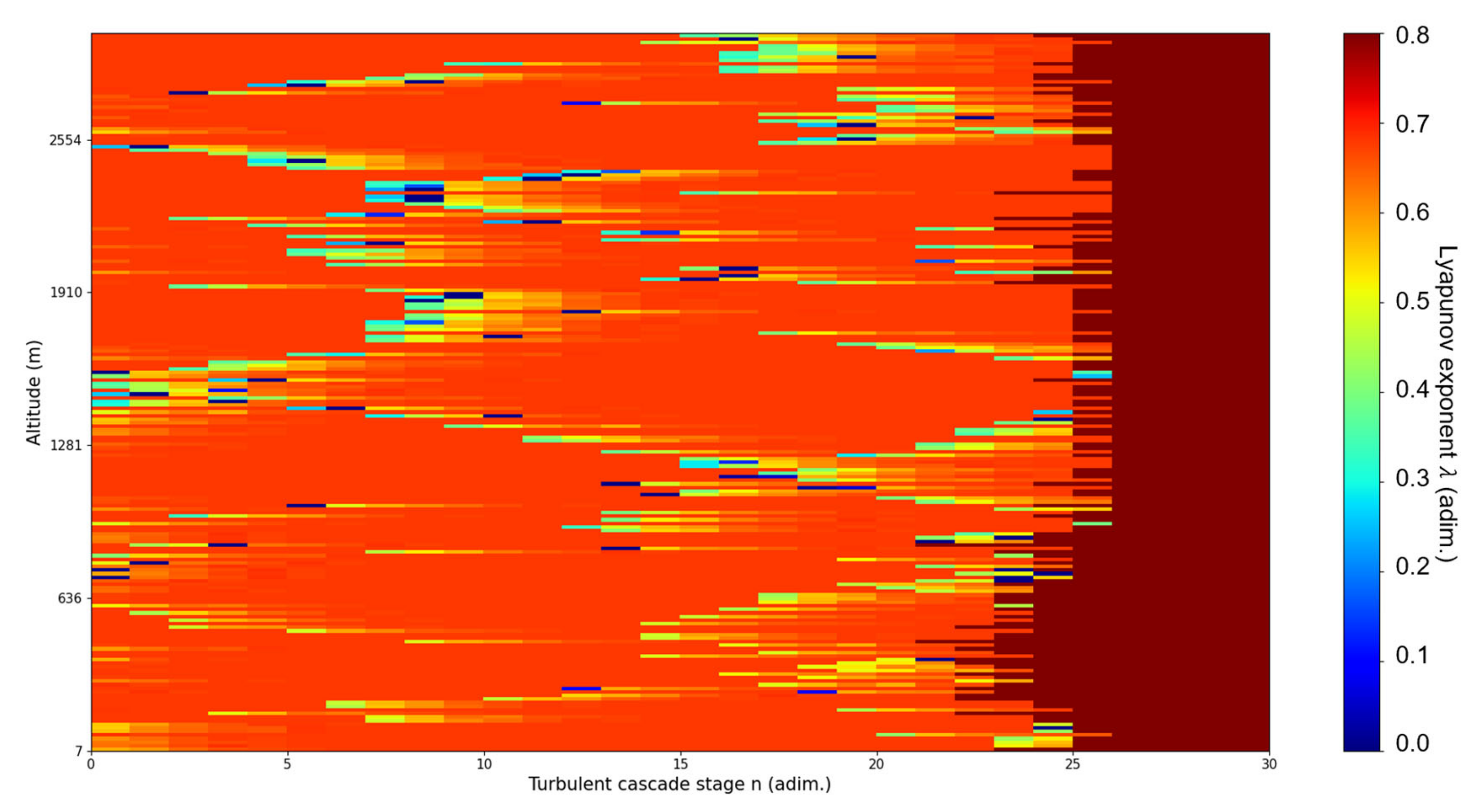
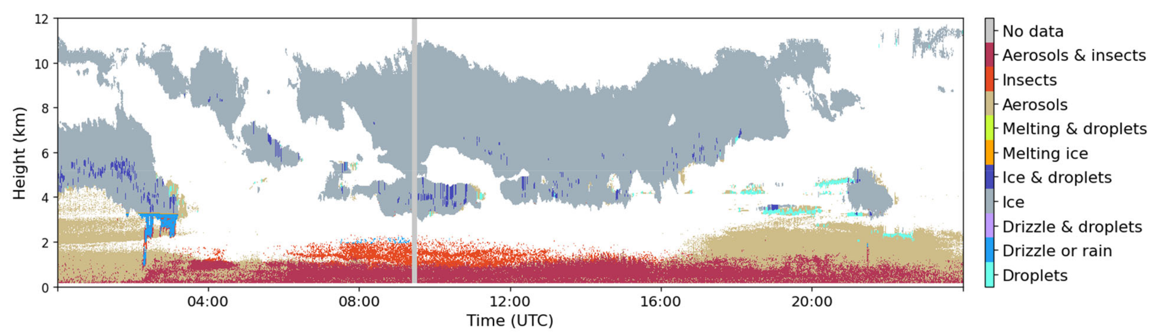
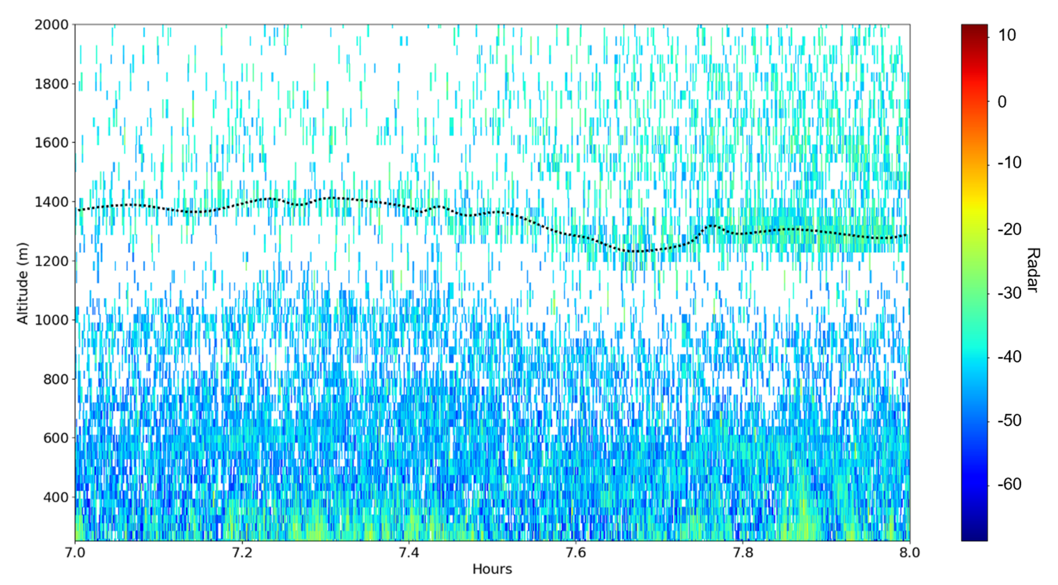
In Figure 2, various data categorizations are performed through ceilometer and radiometer data, and while many types of parameters and atmospheric features can be highlighted through ceilometer and radar data, what interests us in both cases are the vertical insect dynamics. This particular set of data was collected on 4 May 2023.

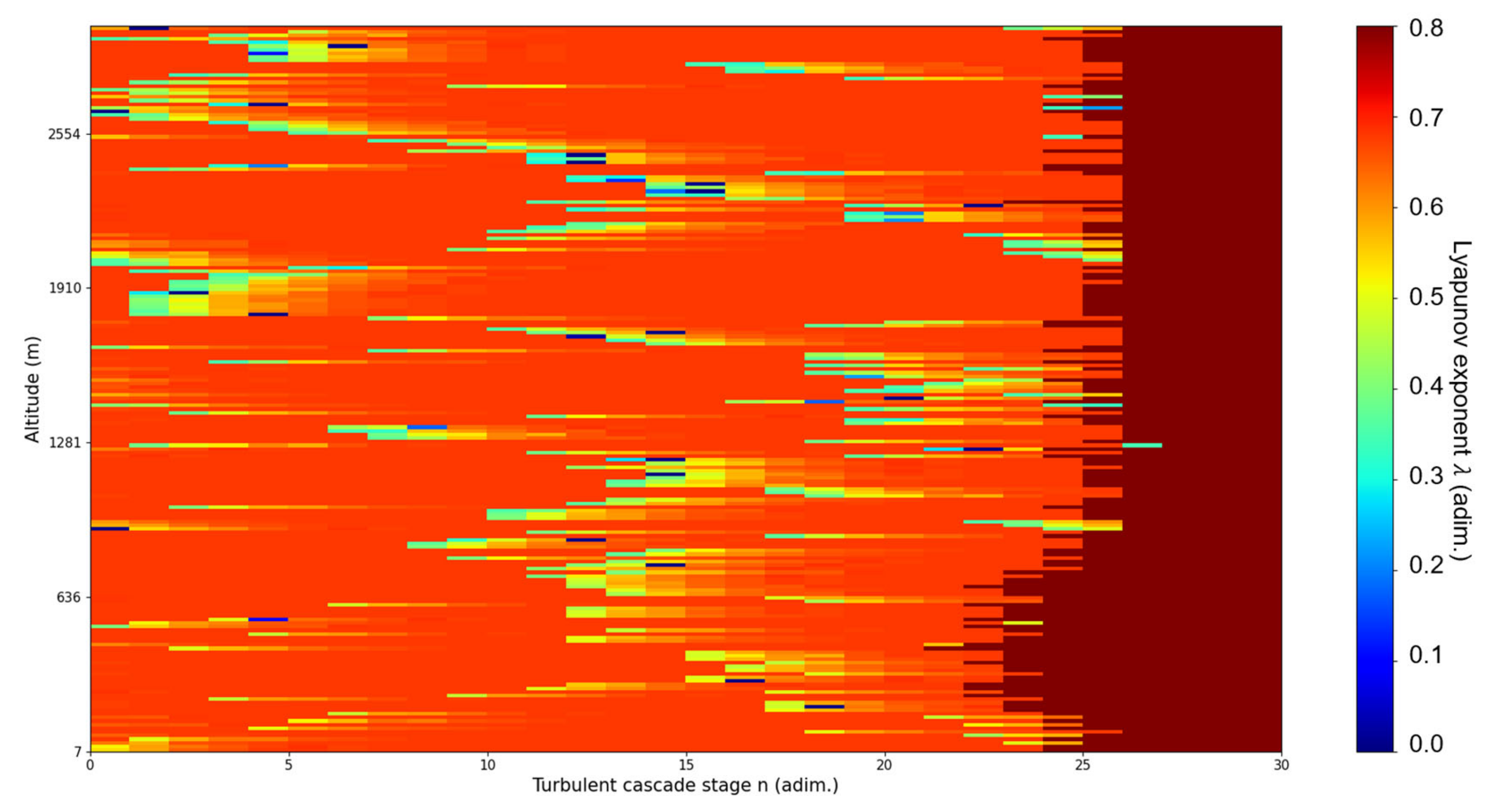
Figure 3 is a zoomed-in version of the region of interest in Figure 2. For this region, laminar plot analysis will be performed every 10 min.

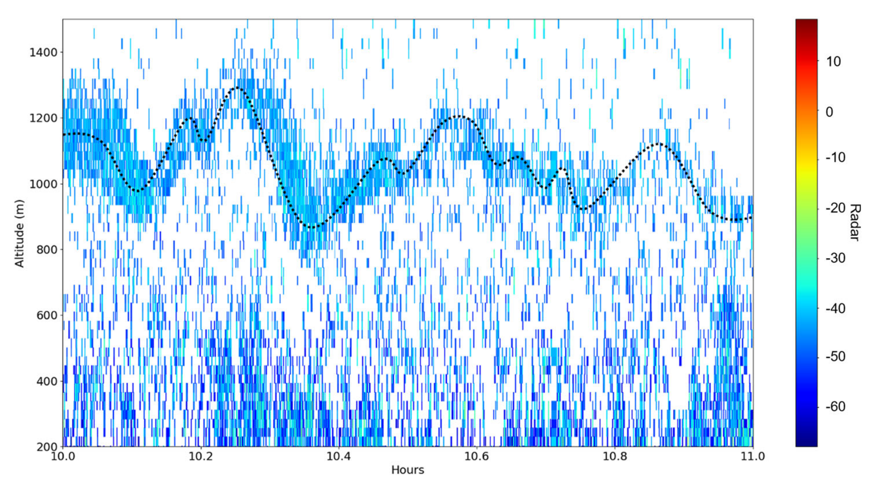
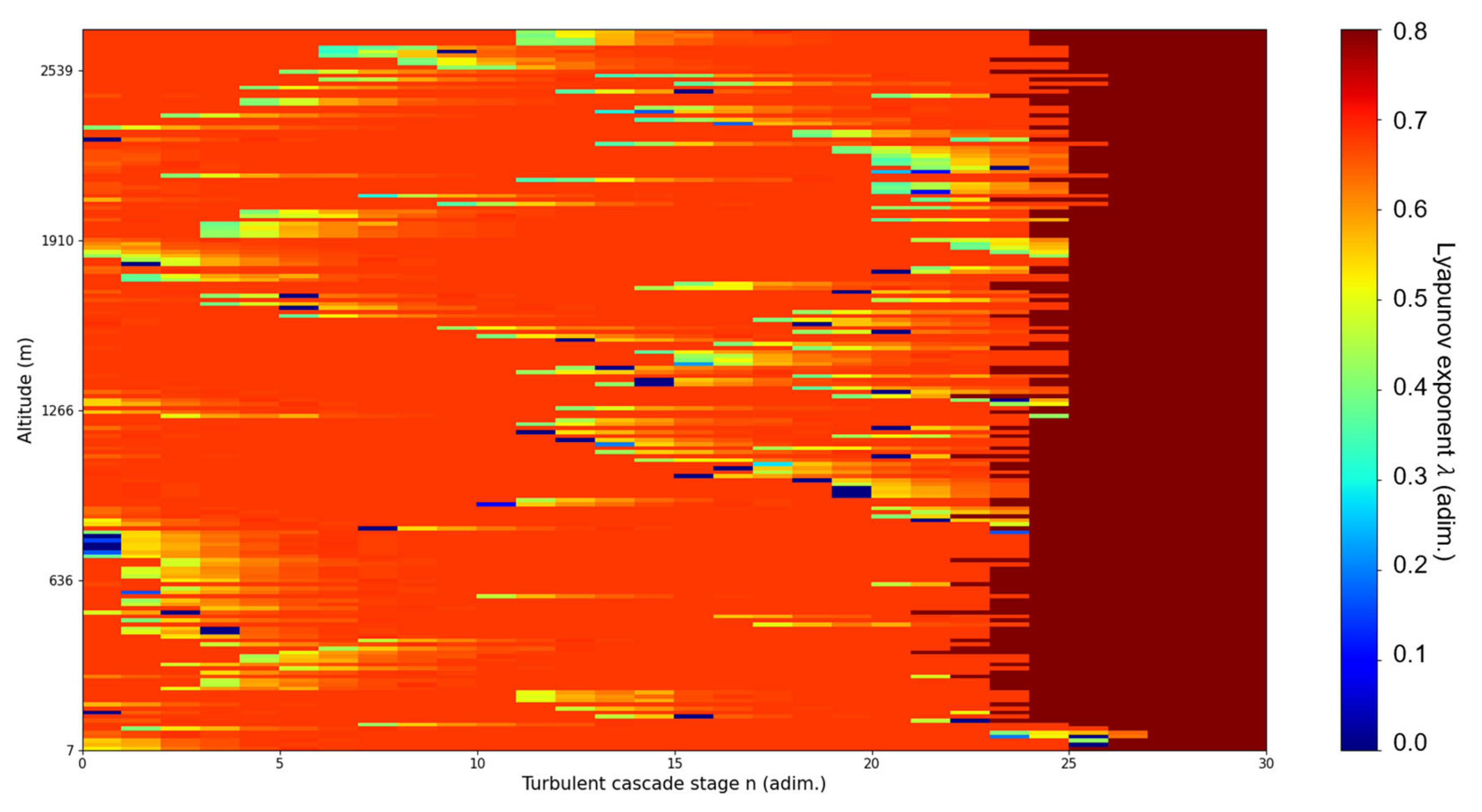
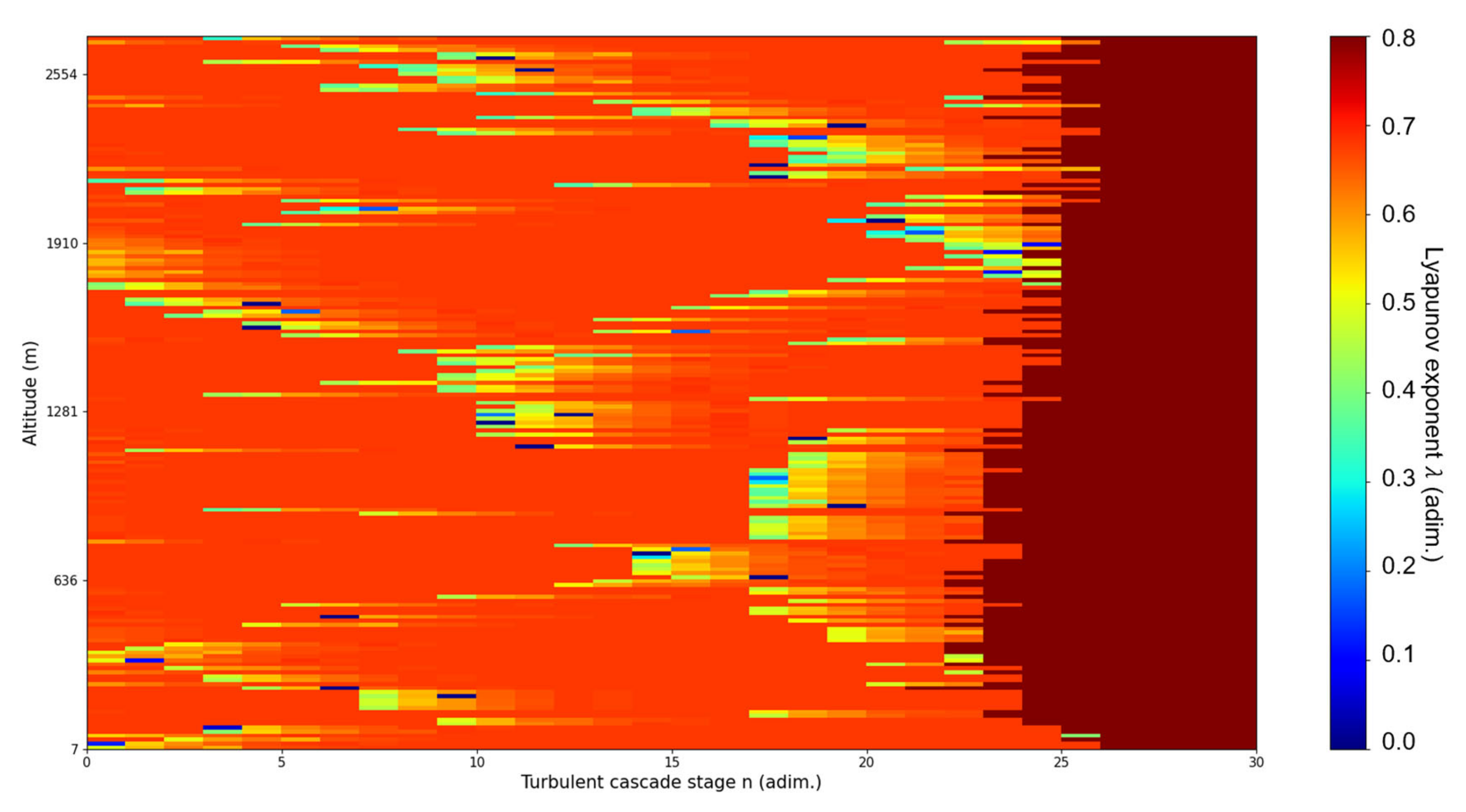
10:00: Laminar channels show uncertainty and a weak descending laminar channel (Figure 4). The insect swarm remains at the same altitude and then shortly after descends (Figure 4). Overall, there is a strong correlation.

10:10: Laminar channels show uncertainty yet overall strong ascendency (Figure 5). The insect swarm fluctuates and then shortly after ascends (Figure 5). Overall, there is a strong correlation.

10:20: Laminar channels show uncertainty (Figure 6). The insect swarm is in a post-descent and pre-ascent state (Figure 6). Overall, there is a strong correlation.

10:30: Laminar channels show uncertainty (Figure 7). The insect swarm is in a post-descent and pre-ascent state (Figure 7). Overall, there is a strong correlation.

10:40: Laminar channels show weak ascendency (Figure 8). The insect swarm is in an instability area and weak ascendency (Figure 8). Overall, there is a strong correlation.

10:50: Laminar channels show uncertainty (Figure 9). The insect swarm is in a post-ascent state (Figure 9). Overall, there is a weak correlation.

11:00: Laminar channels are somewhat uncertain at a chosen altitude and a relatively uncertain state (Figure 10). The insect swarm in a vertically static state (Figure 10). Overall, there is a weak correlation.

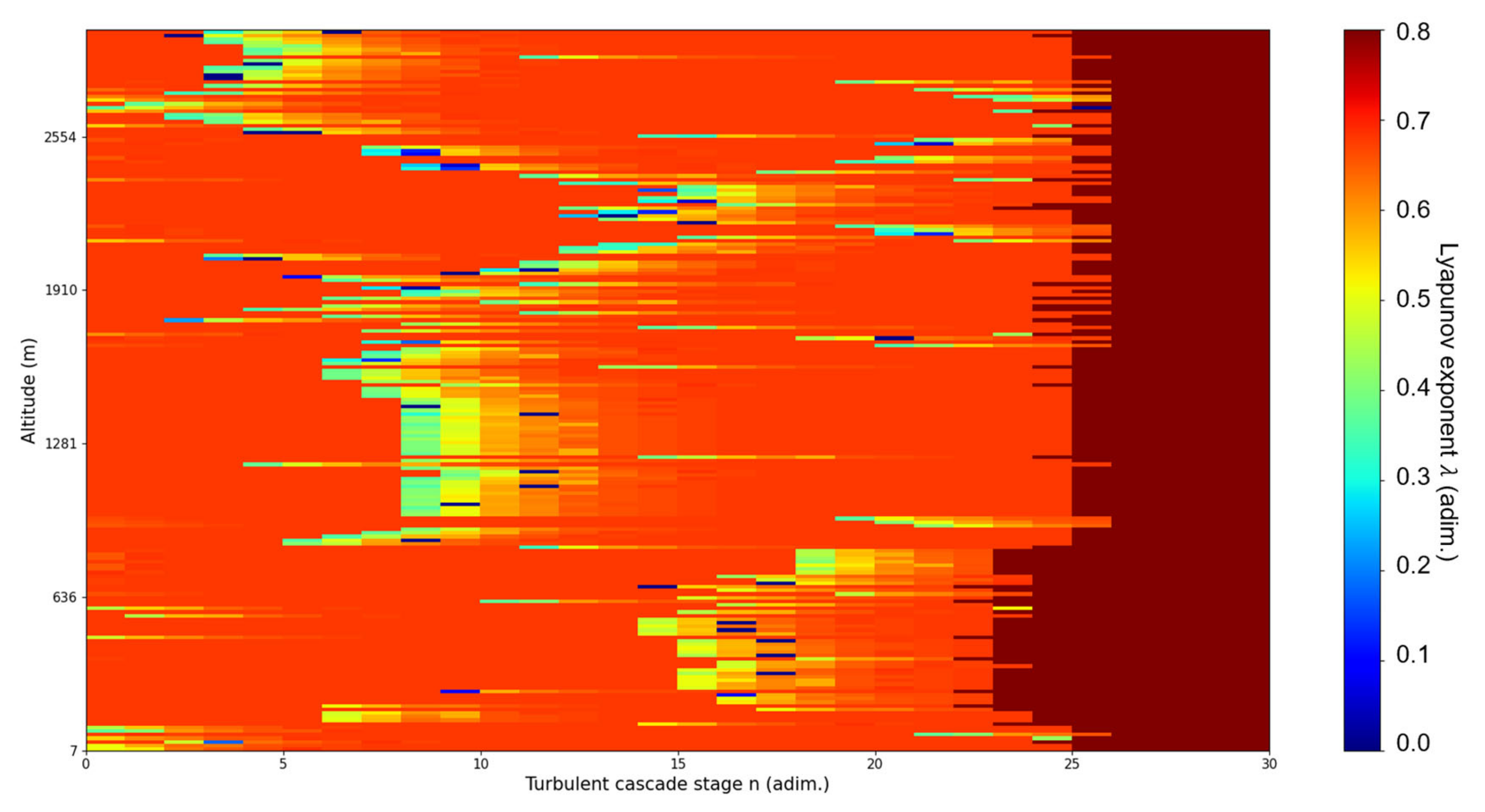
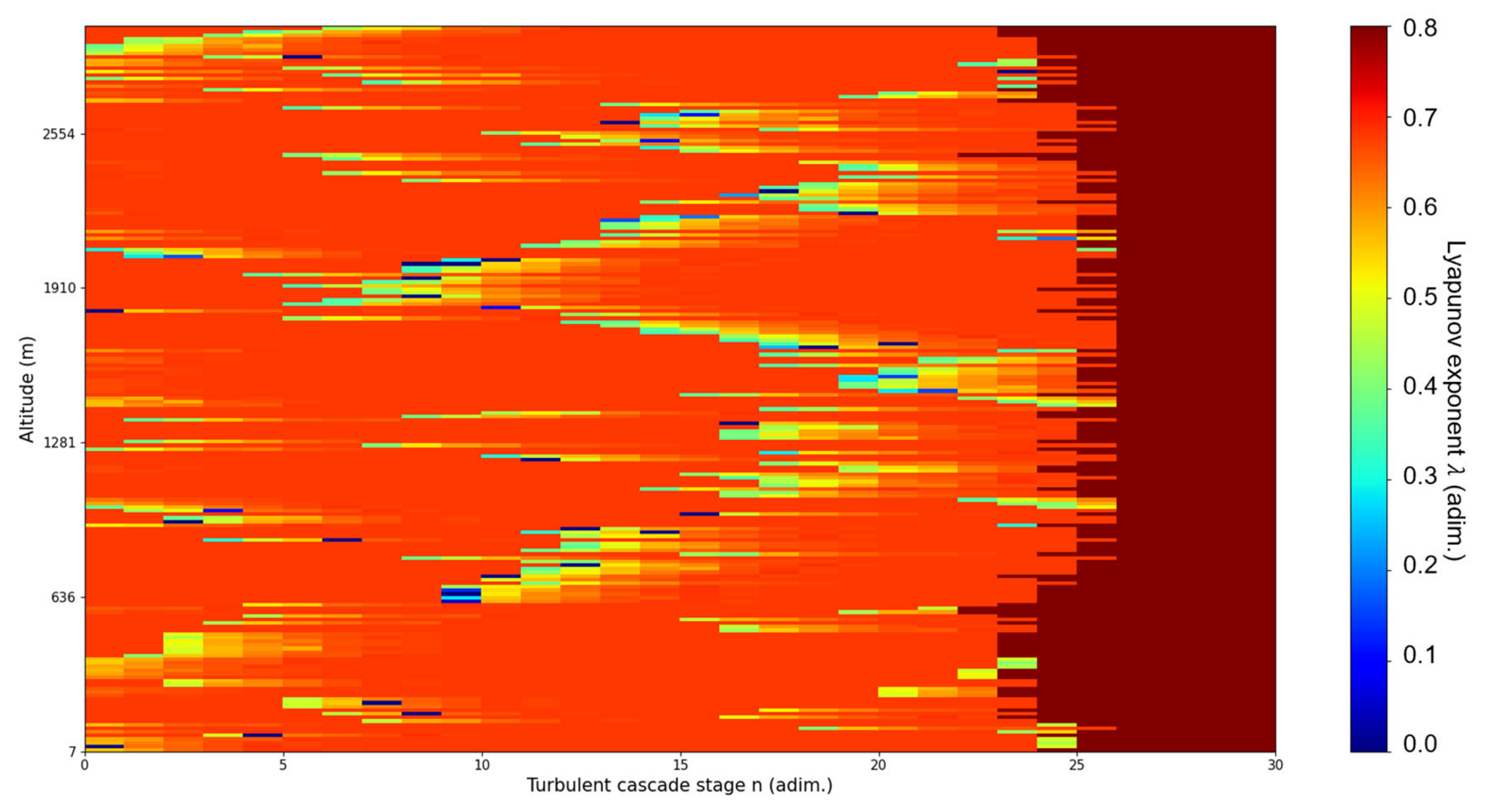
In Figure 11, once again, it is possible to view various data categorizations performed through ceilometer and radiometer data, but vertical insect dynamics are investigated. This particular set of data was collected on 3 May 2023.

Figure 12 is a zoomed-in version of the region of interest in Figure 11. For this region, laminar plot analysis will be performed every 10 min.

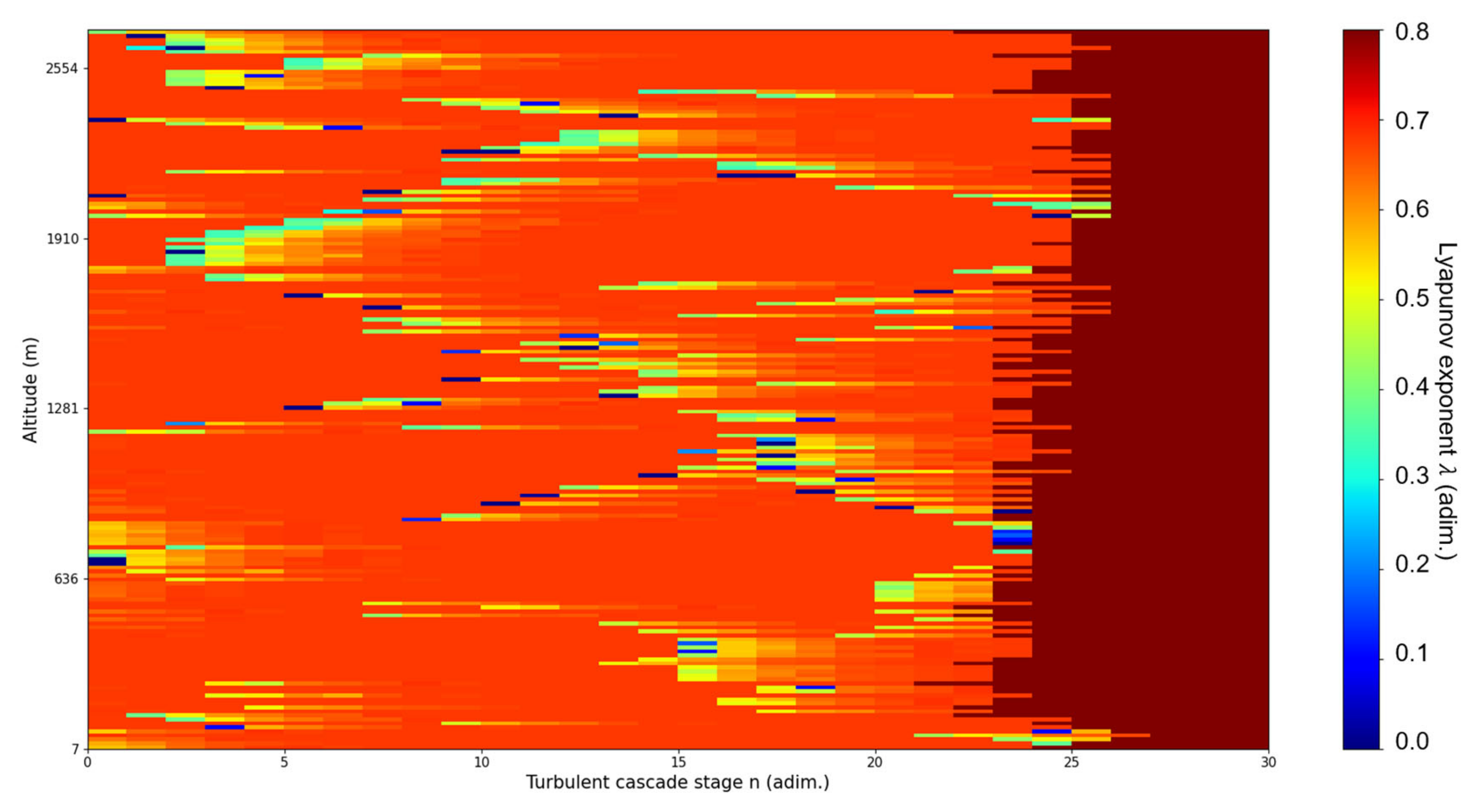
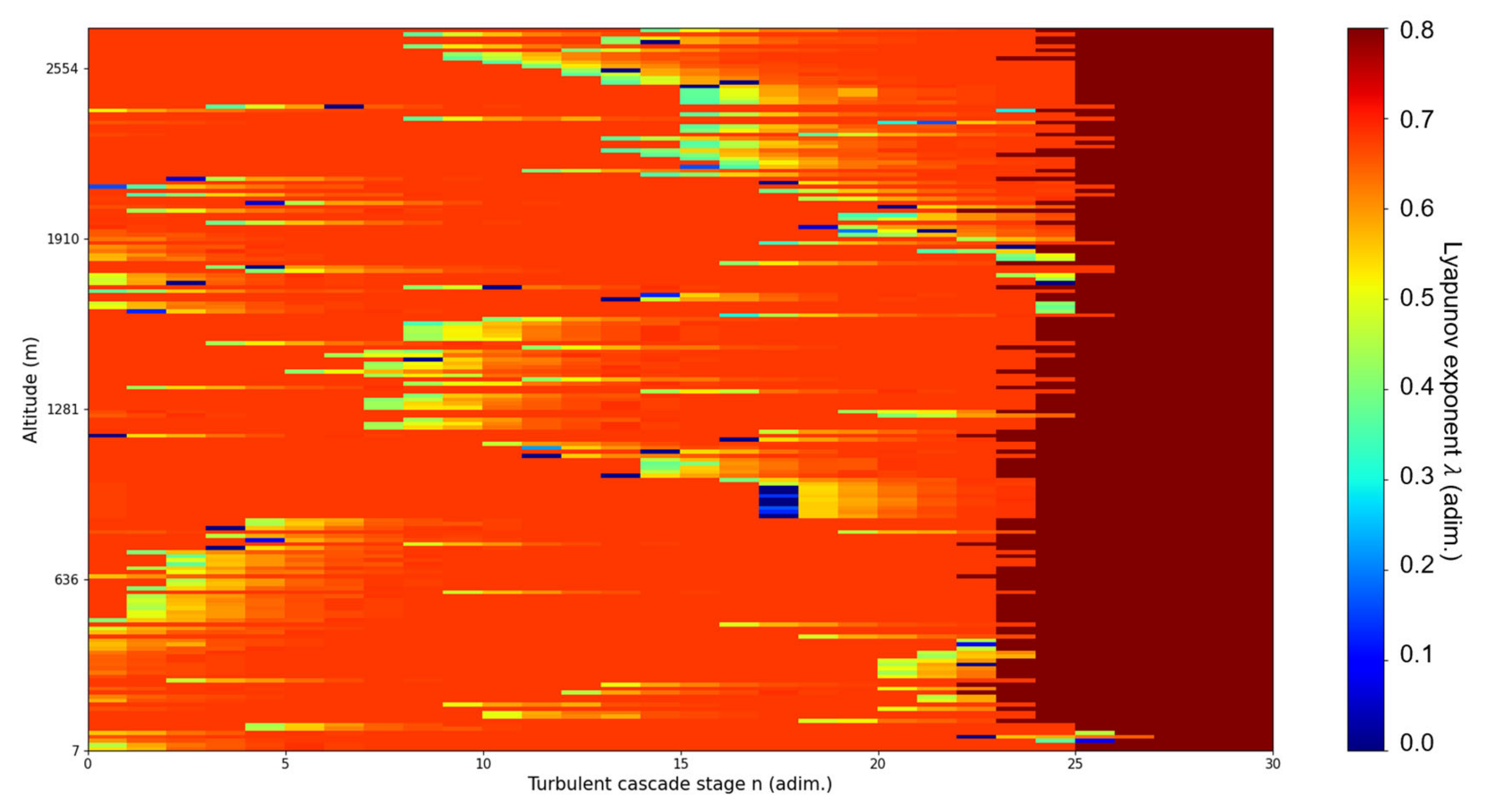
07:00: Laminar channels show uncertainty (Figure 13). The insect swarm remains at the same altitude (Figure 13). Overall, there is a strong correlation.

07:10: Laminar channels show weak ascension and uncertainty lower than the targeted altitude (Figure 14). The insect swarm manifests slow ascension (Figure 14). Overall, there is a strong correlation.

07:20: Laminar channels show descendent behavior at the targeted altitude (Figure 15). The insect swarm manifests slow descent (Figure 15). Overall, there is a strong correlation.

07:30: Laminar channels show uncertainty (Figure 16). The insect swarms are in a weak post-ascent and pre-descent state (Figure 16). Overall, there is a strong correlation.

07:40: Laminar channels show uncertainty at chosen altitude (Figure 17). The insects are in a post-descent state (Figure 17). Overall, there is a strong correlation.

07:50: Laminar channels show uncertainty (Figure 18). The insect swarm remains at the same altitude (Figure 18). Overall, there is a strong correlation.

08:00: Laminar channels show uncertainty (Figure 19). The insect swarm remains at the same altitude (Figure 19). Overall, there is a strong correlation.

Of the 14 cases analyzed in this study, 12 were found to present high correlation, and only 2 were found to present low correlation. Combined with the fact that the analysis was performed with ceilometer data, yet the dynamics were found to be correlated with what can be extracted from radar data, it can be safely stated that the results of our analysis are promising. They show that atmospheric dynamics of any and all physical entities in the atmosphere, including insect swarms, can be modeled using multifractal theories and that these entities follow laminar channels which act to suppress the atmospheric energy dissipation, acting as mass superconducting elements. These results are novel, as they are the first application of laminar analysis outside the vertical dynamics of aerosols, as referenced in our previous works on the subject, and they show that laminar channel analysis can be applied in a variety of cases for the short-term prediction of atmospheric vertical dynamics. The accurate short-term prediction of such dynamics is important in a myriad of cases regarding pollution control and meteorology, and in the case of insect swarms, such platforms could be successfully used in many agricultural applications.

7. Conclusions

In conclusion, a multifractal interpretation of the atmosphere was presented, and it was found that such interpretations, through Schrödinger and Madelung-type scenarios and Riccati-type gauges, lead to digital behaviors in the atmospheric behavior of turbulence, such as modulation and discretization. These behaviors can be syncretized with other previously studied characteristics of the multifractal atmosphere, such as the emergence of laminar channels and the interpretation of the atmosphere through mass conduction, and many theoretical similarities are found. Most importantly, it is found that through these theories, it is established that laminar channels throughout the atmosphere act as a mass superconducting medium. Finally, experimental data from a ceilometer and radar platform is used in order to confirm the theory, in the case of vertical insect swarm dynamics, with satisfactory results. Future studies in this direction might further use more data in the service of such analyses for the purpose of greater experimental correlation and verification, and such studies could also focus on automating future algorithms for such platforms in the interest of more common uses.