
An Operational Approach to Fractional Scale-Invariant Linear Systems


Abstract
:1. Introduction
2. Scale–Invariant Systems and Derivatives
2.1. The Mellin Convolution
- piecewise continuous,
- with bounded variation.
2.2. Scale-Derivatives
2.2.1. Stretching Derivatives: [16]
2.2.2. Shrinking Derivatives: [16]
- Hadamard–Liouville left derivative [16]
2.3. ARMA Type Systems
3. The Algebraic Framework for Solving DI-FARMA Systems
3.1. Sequence of Basic Functions for Fractional Scale Derivatives
Hadamard Right (Left) Derivative
3.2. The Framework
- is the neutral element of the Mellin convolution, ;
- the inverse element of is , .
- Derivative on a parameterwhere means usual derivative with respect to .
- Convolution of two different –log-exponential functions, but with the same parameter
- Convolution of two different parameters –log-exponential functionsFor ,
4. Impulse and Step Responses
4.1. The AR Case
4.2. The ARMA Case
5. Examples
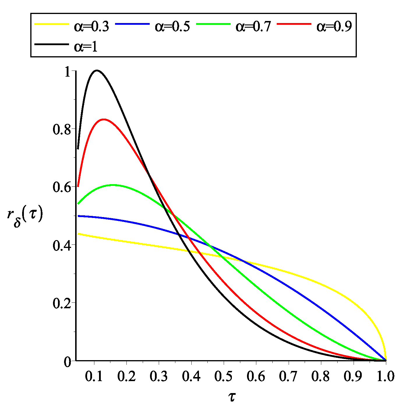
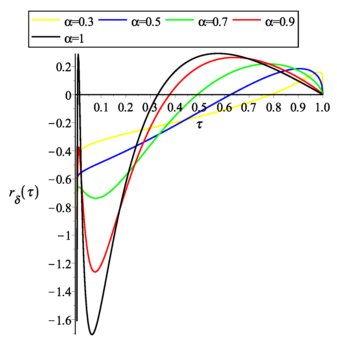
- Operational method:By means of our operational method, the system can be rewritten asWe propose the solutionFollowing the presented in Section 3.2 we obtain the system of equationsThe solution to system of equations is and . Therefore, for the impulse response isand step responseRemark 7.When , and .The Figure 1 and Figure 2 show the graphical representation of the solutions with and several values of α.For , the impulse response isand step responseRemark 8.When ,and
- Mellin transform:
6. Conclusions
Author Contributions
Funding
Conflicts of Interest
Appendix A
Appendix B
References
- Roberts, M.J. Signals and Systems: Analysis Using Transform Methods and Matlab; McGraw-Hill: New York, NY, USA, 2003. [Google Scholar]
- Shmaliy, Y. Continuous-Time Systems; Springer Science & Business Media: Berlin/Heidelberg, Germany, 2007. [Google Scholar]
- Braccini, C.; Gambardella, G. Form-invariant linear filtering: Theory and applications. IEEE Trans. Acoust. Speech Signal Process. 1986, 34, 1612–1628. [Google Scholar] [CrossRef]
- Yazici, B.; Kashyap, R. A class of second-order stationary self-similar processes for 1/f phenomena. IEEE Trans. Signal Process. 1997, 45, 396–410. [Google Scholar] [CrossRef]
- Ortigueira, M.D. On the fractional linear scale invariant systems. IEEE Trans. Signal Process. 2010, 58, 6406–6410. [Google Scholar] [CrossRef]
- Nottale, L. The theory of scale relativity. Int. J. Mod. Phys. A 1992, 7, 4899–4936. [Google Scholar] [CrossRef] [Green Version]
- Narasimha, R.; Rao, R. Modeling variable-bit-rate video traffic using linear scale-invariant systems. In Wavelet and Independent Component Analysis Applications IX; SPIE: Bellingham, WA, USA, 2002; Volume 4738, pp. 79–89. [Google Scholar]
- Cresson, J. Scale relativity theory for one-dimensional non-differentiable manifolds. Chaos Solitons Fractals 2002, 14, 553–562. [Google Scholar] [CrossRef] [Green Version]
- Cresson, J. Scale calculus and the Schrödinger equation. J. Math. Phys. 2003, 44, 4907–4938. [Google Scholar] [CrossRef] [Green Version]
- Khaluf, Y.; Ferrante, E.; Simoens, P.; Huepe, C. Scale invariance in natural and artificial collective systems: A review. J. R. Soc. Interface 2017, 14, 20170662. [Google Scholar] [CrossRef] [PubMed] [Green Version]
- Rao, R.; Zhao, W. Image modeling with linear scale-invariant systems. In Wavelet Applications VI; SPIE: Bellingham, WA, USA, 1999; Volume 3723, pp. 407–418. [Google Scholar]
- Gorenflo, R.; Luchko, Y.; Mainardi, F. Wright functions as scale-invariant solutions of the diffusion-wave equation. J. Comput. Appl. Math. 2000, 118, 175–191. [Google Scholar] [CrossRef] [Green Version]
- Herrmann, R. Fractional Calculus: An Introduction for Physicists; World Scientific: Singapore, 2014. [Google Scholar]
- Hirschman, I.I.; Widder, D.V. The Convolution Transform; Courier Corporation: Honolulu, HI, USA, 2012. [Google Scholar]
- Poularikas, A. The Transforms and Applications Handbook; CRC Press LLC: Boca Raton, FL, USA, 2000. [Google Scholar]
- Ortigueira, M.; Bohannan, G. Fractional Scale Calculus: Hadamard vs. Liouville. Fractal Fract. 2023, 7, 296. [Google Scholar] [CrossRef]
- Samko, S.; Kilbas, A.; Marichev, O. Fractional Integrals and Derivatives; Gordon and Breach: New York, NY, USA, 1993. [Google Scholar]
- Ortigueira, M.; Valério, D. Fractional Signals and Systems; De Gruyter: Berlin, Germany, 2020. [Google Scholar]
- Ortigueira, M.D.; Machado, J.T. The 21st century systems: An updated vision of continuous-time fractional models. IEEE Circuits Syst. Mag. 2022, 22, 36–56. [Google Scholar] [CrossRef]
- Bengochea, G.; Ortigueira, M. An operational approach to solve fractional continuous–time linear systems. Int. J. Dyn. Control 2017, 5, 61–71. [Google Scholar] [CrossRef]
- Butzer, P.; Jansche, S. A direct approach to the Mellin transform. J. Fourier Anal. Appl. 1997, 3, 325–376. [Google Scholar] [CrossRef]
- Luchko, Y.; Kiryakova, V. The Mellin integral transform in fractional calculus. Fract. Calc. Appl. Anal. 2013, 16, 405–430. [Google Scholar] [CrossRef]
- Hadamard, J. Essai sur l’étude des fonctions données par leur développement de Taylor. J. Math. Pures Appl. 1892, 8, 101–186. [Google Scholar]
- Kilbas, A.; Srivastava, H.; Trujillo, J. Theory and Applications of Fractional Differential Equations; North-Holland Mathematics Studies; Elsevier: Amsterdam, The Netherlands, 2006; Volume 204. [Google Scholar]
- Ortigueira, M.; Bengochea, G.; Machado, J. Substantial, tempered, and shifted fractional derivatives: Three faces of a tetrahedron. Math. Methods Appl. Sci. 2021, 44, 9191–9209. [Google Scholar] [CrossRef]
- Ortigueira, M.; Bengochea, G. Non-commensurate fractional linear systems: New results. J. Adv. Res. 2020, 25, 11–17. [Google Scholar] [CrossRef] [PubMed]
- Appell, P. Sur une classe de polynômes. Ann. Sci. de l’École Norm. Supérieure. 1880, 9, 119–144. [Google Scholar] [CrossRef] [Green Version]
- Rota, G.; Taylor, B. The classical umbral calculus. SIAM J. Math. Anal. 1994, 25, 694–711. [Google Scholar] [CrossRef]
- Roman, S. The Umbral Calculus; Springer: Berlin/Heidelberg, Germany, 2005. [Google Scholar]
- Gel’fand, I.; Shilov, G. Generalized Functions; Academic Press: Cambridge, MA, USA, 1964. [Google Scholar]
- Bengochea, G.; Verde-Star, L. Linear algebraic foundations of the operational calculi. Adv. Appl. Math. 2011, 47, 330–351. [Google Scholar] [CrossRef] [Green Version]
- Verde-Star, L. Inverses of generalized Vandermonde matrices. J. Math. Anal. Appl. 1988, 131, 341–353. [Google Scholar] [CrossRef] [Green Version]


Disclaimer/Publisher’s Note: The statements, opinions and data contained in all publications are solely those of the individual author(s) and contributor(s) and not of MDPI and/or the editor(s). MDPI and/or the editor(s) disclaim responsibility for any injury to people or property resulting from any ideas, methods, instructions or products referred to in the content. |
© 2023 by the authors. Licensee MDPI, Basel, Switzerland. This article is an open access article distributed under the terms and conditions of the Creative Commons Attribution (CC BY) license (https://creativecommons.org/licenses/by/4.0/).
Share and Cite
Bengochea, G.; Ortigueira, M.D. An Operational Approach to Fractional Scale-Invariant Linear Systems. Fractal Fract. 2023, 7, 524. https://doi.org/10.3390/fractalfract7070524
Bengochea G, Ortigueira MD. An Operational Approach to Fractional Scale-Invariant Linear Systems. Fractal and Fractional. 2023; 7(7):524. https://doi.org/10.3390/fractalfract7070524
Chicago/Turabian StyleBengochea, Gabriel, and Manuel Duarte Ortigueira. 2023. "An Operational Approach to Fractional Scale-Invariant Linear Systems" Fractal and Fractional 7, no. 7: 524. https://doi.org/10.3390/fractalfract7070524