Investigating Families of Soliton Solutions for the Complex Structured Coupled Fractional Biswas–Arshed Model in Birefringent Fibers Using a Novel Analytical Technique

Abstract

This research uses a novel analytical method known as the modified Extended Direct Algebraic Method (mEDAM) to explore families of soliton solutions for the complex structured Coupled Fractional Biswas–Arshed Model (CFBAM) in Birefringent Fibers. The Direct Algebraic Method (DAM) is extended by the mEDAM’s methodology to compute more analytical solutions that would otherwise be difficult to acquire. We use this method to derive several families of soliton solutions and examine their characteristics. We also look at how different model parameters, such as amplitude, width, and propagation speed, affect the dynamics of soliton. Our use of 2D and 3D graphics to illustrate the soliton solutions also makes it possible to see the soliton dynamics more clearly. The outcomes also demonstrate that the method suggested has proven successful in producing soliton solutions for intricate structures such as the CFBAM.

1. Introduction

In order to model complex physical phenomena with non-classical and non-local effects such as long-range interactions and fractal materials, Fractional Partial Differential Equations (FPDEs) have become a promising mathematical tool. As compared to conventional Partial Differential Equations (PDEs), FPDEs provide a more precise and thorough description of such complex processes, making them an important tool for researchers in the fields of physics, engineering, and other sciences [1,2,3,4]. Because of this, FPDEs are being used more often in scientific research. This has made it easier to create new theoretical frameworks and experimental plans that can better capture the complex behaviors of natural systems [5,6,7,8,9].

The CFBAM expands the complex structured Coupled Biswas–Arshed Model (CBAM) by including fractional temporal derivatives as well as second- and third-order temporal-spatial dispersion [10]. By taking into consideration the effects of Group Velocity Dispersion (GVD), Polarization Mode Dispersion (PMD), self-phase modulation, and higher-order dispersion, this model properly depicts soliton propagation in birefringent fibers. Short Term Dispersion (STD) (which results from changes in the fiber’s refractive index over brief distances) is also taken into account by the model. Polarization controllers or polarization-maintaining fibers can be used to account for the soliton propagation in birefringent fibers. The CFBAM has significant uses in optical communication systems for long-distance and high-speed data transfer [11].

Since non-local and memory effects cannot be accounted by conventional integer-order differential equations, it is advantageous to consider the CBAM in fractional form. This could give modelers of complicated processes with long-term memory effects a more flexible and broad framework. The CFBAM can more accurately depict the soliton wave propagation in birefringent fibers by using fractional temporal and spatial derivatives, particularly in the presence of high degrees of dispersion and noise. The design and improvement of optical communication systems for high-speed data transfer over vast distances can benefit greatly from the use of this model. In the current investigation, the CFBAM is taken into account in the form of two vector polarity components in birefringent fibers without Four Wave Mixing (FWM) factors. The FBAM without FWM in the birefringent fibers is given as:

$$\begin{array}{cc}\hfill & i{u}_t^{\alpha }+a_1{u}_{xx}^{2\beta }+b_1{u}_{xt}^{\alpha \beta }+i(c_1{u}_{xxx}^{3\beta }+e_1{u}_{xxt}^{\alpha 2\beta })=i\left[\right({\lambda }_1{(\mid u{\mid }^{2}u)}_x^{\beta }\hfill \\ \hfill & +{\gamma }_1{(\mid v{\mid }^{2}v)}_x^{\beta }]+i[{\mu }_1{(\mid u{\mid }^2)}_x^{\beta }+{\alpha }_1{(\mid v{\mid }^2)}^{\beta }x]u+i[{\theta }_1\mid u{\mid }^2+{\tau }_1\mid v{\mid }^2]u_x^{\beta },\hfill \end{array}$$

(1)

$$\begin{array}{cc}\hfill & i{v}_t^{\alpha }+a_2{v}_{xx}^{2\beta }+b_2{v}_{xt}^{\alpha \beta }+i(c_2{v}_{xxx}^{3\beta }+e_2{v}_{xxt}^{\alpha 2\beta })=i\left[\right({\lambda }_2{(\mid v{\mid }^{2}v)}_x^{\beta }\hfill \\ \hfill & +{\gamma }_2{(\mid u{\mid }^{2}u)}_x^{\beta }]+i[{\mu }_2{(\mid v{\mid }^2)}_x^{\beta }+{\alpha }_2(\mid u{\mid }^2)x]v+i[{\theta }_2\mid v{\mid }^2+{\tau }_2\mid u{\mid }^2]v_x^{\beta },\hfill \end{array}$$

(2)

where $0<\alpha ,\beta \le 1$, $u=u(x,t)$ & $v=v(x,t)$. The first terms in (1) and (2) are referred to as the temporal development of pulses. The coefficients $a_k$ and $b_k,(k=1,2)$ give evidence for the existence of GVD and STD. The coefficients $c_k$ and $e_k$, respectively, ensure the presence of third order STD and third-order temporal dispersion (3OD). The coefficients of ${\lambda }_k$, ${\gamma }_k$, ${\mu }_k$, ${\alpha }_k$, ${\theta }_k$, and ${\tau }_k$ ensure the nonlinear terms that show nonlinear dispersion and self-steepening.

Due to their non-local and non-classical nature, FPDEs are difficult to be solved analytically. Even though analytical methods offer more precise results and in-depth understanding of the underlying physical processes, they might not always be available or simple to use in order to solve FPDEs. In these situations, the solutions are approximated using numerical techniques including the finite difference method [12], finite element method [13], and wavelet operational method [14]. However, compared to analytical approaches, numerical methods have some drawbacks, such as error from discretization and rounding, a lack of closed-form solutions, problems with stability and convergence, and high computing costs for big or complicated problems. Numerical solutions may also be challenging to comprehend in the absence of a closed-form solution, while convergence and stability problems necessitate careful method selection and testing. Therefore, analytical techniques such as the Fractional Differential Transform Method (FDTM) [15], Variational Iteration Method (VIM) [16], (G′/G)-expansion method [17], tan-expansion method [18], exp-function method [19], mEDAM [20] and many others [21,22,23,24,25] are created to tackle the complexity of FPDEs and provide distinct benefits over numerical techniques.

Among these analytical techniques, a novel technique called the mEDAM may be utilized to find families of solitons solutions for FPDEs. mEDAM uses a variable transformation to convert the FPDE into nonlinear Ordinary Differential Equations (ODE). The nonlinear ODE is then transformed into a set of algebraic equations using the supposition of a series form solution. The soliton solutions for the desired FPDEs can be obtained by solving the ensuing system of algebraic equations. The mEDAM can manage the non-local and non-classical character of these equations, making it particularly helpful for FPDEs that are challenging to solve with traditional analytical techniques. The soliton solutions obtained by mEDAM can also provide light on the system’s behavior and aid in a better understanding of the underlying physical processes.

The goal of this research is to retrieve a novel soliton solution for the CFBAM in birefringent fibers. Before this research work, mathematicians have addressed this model using different analytical methods; for example, Li [26] explored the BA model, acquired optical soliton solutions, and produced phase portraits. Similarly, the stated model with beta derivative was examined by Ozkan [27], who used the simplest equation technique and an extended hyperbolic auxiliary approach to discover optical soliton solutions. In [28], the BA model with beta derivative was subjected by Zafar et al. to the expanded Sinh–Gordon expansion and the modified expansion processes in order to obtain optical solutions. On the other hand, the optical solutions were obtained by Hosseini [29] using the Jacobi and Kudryashov techniques from the BA model with beta derivative. Demiray [30] examined solitary waves for the given model using the generalized Kudryashov approach. Similarly, Shiekh et al. utilized Jacobi’s elliptic function approach to address CBAM in integer orders [10].

The fractional derivatives present in (1) and (2) are defined in Caputo’s sense. This derivative’s operator for a smooth function $f(x,t)$ is defined as [31]:

$$D_y^{\alpha }z(x,y)=\left\{\begin{array}{c}\frac{1}{\Gamma (1-\alpha )}{\int }_0^y\frac{\partial }{\partial \rho }z(x,\rho ){(\rho -y)}^{-\alpha }d\rho ,\alpha \in (0,1)\hfill \\ \frac{\partial z(x,y)}{\partial t},\alpha =1\hfill \end{array}\right.$$

(3)

The FPDEs in (1) and (2) are converted into NODEs using the derivative’s two following properties:

$$D_{\zeta }^r{\zeta }^k=\frac{\Gamma (1+k)}{\Gamma (1+k-r)}{\zeta }^{k-r},$$

(4)

$$D_{\zeta }^{\alpha }y\left[x\left(\zeta \right)\right]=y_x^{\prime }\left(x\left(\zeta \right)\right)D_{\zeta }^{\alpha }x\left(\zeta \right)=D_x^{\alpha }y\left(x\left(\zeta \right)\right){\left[x^{\prime }\left(\zeta \right)\right]}^{\alpha },$$

(5)

where k is a real number and $y\left(\zeta \right)$ and $x\left(\zeta \right)$ represent arbitrary functions that are differentiable.

2. The Methodology of Modified EDAM [32]

In this section, we outline the mEDAM technique. Consider the FPDE of the form:

$$E(\Psi ,{\partial }_t^{\rho }\Psi ,{\partial }_{{\phi }_1}^{\varrho }\Psi ,{\partial }_{{\phi }_2}^{\sigma }\Psi ,\Psi {\partial }_{{\phi }_1}^{\beta }\Psi ,\dots )=0,0<\rho ,\varrho ,\sigma \le 1,$$

(6)

where $\Psi =\Psi (t,{\phi }_1,{\phi }_2,{\phi }_3,\dots ,{\phi }_n)$.

The following steps are used to solve (6):

• First, we carry out a variable transformation $\Psi (t,{\phi }_1,{\phi }_2,{\phi }_3,\dots ,{\phi }_n)=\theta (\Phi )$, $\Phi =\Phi (t,{\phi }_1,{\phi }_2,{\phi }_3,\dots ,{\phi }_n)$, where there are several ways to describe $\Phi$.
  Thus, (6) is changed by this transformation to a nonlinear ODE of the following form:

  $$F(\theta ,{\theta }^{\prime },\theta {\theta }^{\prime },\dots )=0,$$

  (7)

  where $\theta$ in (7) has derivatives with respect to $\Phi$. Sometimes, the constant(s) of integration may then be obtained by integrating (7) a single time or more.
• Then, we assume that (7) has the following solution:

  $$\theta (\Phi )=\sum _{j=-b_1}^{b_1}{a}_j{\left(Y(\Phi )\right)}^j,$$

  (8)

  where $a_j(l=-b_1,\dots ,0,1,2,\dots ,b_1)$ are unknown constants to be estimated later, and $Y(\Phi )$ satisfies the following nonlinear first order ODE:

  $$Y^{\prime }(\Phi )=ln\left(A\right)(c{\left(Y(\Phi )\right)}^2+bY(\Phi )+a),$$

  (9)

  where $c,b,a$ are arbitrary constants and $A\ne 0,1$.
• Finding the homogeneous balance among the greatest nonlinear term and the highest order derivative in (7) yields the positive integer $b_1$ given in (8).
• Next, we plug (8) in (7) or in the integrated form of (7), and then all those terms of $\left(Y\right(\Phi \left)\right)$ which have same orders are assembled, which yields a polynomial in $\left(Y\right(\Phi \left)\right)$. The obtained polynomial’s coefficients are then all set to zero, resulting in a system of algebraic equations for $a_l(l=-b_1,\dots ,0,1,2,\dots ,b_1)$ and additional parameters.
• To resolve this set of algebraic equations, we utilize MAPLE.
• The analytical solutions to Equation (6) are then obtained by determining the unknown parameters and inserting them into Equation (8) together with $Y(\Phi )$ (the solution of Equation (9)). We may create the families of precise soliton solutions shown below using the general solution of (9):

Family 1.

For $P<0$ and $c\ne 0$, the following family of solitary wave solutions is implied by the general solution of (9):

$$Y_1(\Phi )=-\frac{b}{2c}+\frac{\sqrt{-P}{tan}_A\left(1/2\sqrt{-P}\Phi \right)}{2c},$$

$$Y_2(\Phi )=-\frac{b}{2c}-\frac{\sqrt{-P}{cot}_A\left(1/2\sqrt{-P}\Phi \right)}{2c},$$

$$Y_3(\Phi )=-\frac{b}{2c}+\frac{\sqrt{-P}\left({tan}_A\left(\sqrt{-P}\Phi \right)\pm \left(\sqrt{pq}{sec}_A\left(\sqrt{-P}\Phi \right)\right)\right)}{2c},$$

$$Y_4(\Phi )=-\frac{b}{2c}-\frac{\sqrt{-P}\left({cot}_A\left(\sqrt{-P}\Phi \right)\pm \left(\sqrt{pq}{csc}_A\left(\sqrt{-P}\Phi \right)\right)\right)}{2c},$$

and

$$Y_5(\Phi )=-\frac{b}{2c}+\frac{\sqrt{-P}\left({tan}_A\left(1/4\sqrt{-P}\Phi \right)-{cot}_A\left(1/4\sqrt{-P}\Phi \right)\right)}{4c}.$$

Family 2.

For $P>0$ and $c\ne 0$ the following family of solitary wave solutions is implied by the general solution of (9):

$$Y_6(\Phi )=-\frac{b}{2c}-\frac{\sqrt{P}{tanh}_A(1/2\sqrt{P}\Phi )}{2c},$$

$$Y_7(\Phi )=-\frac{b}{2c}-\frac{\sqrt{P}{coth}_A\left(1/2\sqrt{P}\Phi \right)}{2c},$$

$$Y_8(\Phi )=-\frac{b}{2c}-\frac{\sqrt{P}\left({tanh}_A\left(\sqrt{P}\Phi \right)\pm \left(\sqrt{pq}{\sec \mathrm{h}}_A\left(\sqrt{P}\Phi \right)\right)\right)}{2c},$$

$$Y_9(\Phi )=-\frac{b}{2c}-\frac{\sqrt{P}\left({coth}_A\left(\sqrt{P}\Phi \right)\pm \left(\sqrt{pq}{\csc \mathrm{h}}_{\mathit{A}}\left(\sqrt{P}\Phi \right)\right)\right)}{2c},$$

and

$$Y_{10}(\Phi )=-\frac{b}{2c}-\frac{\sqrt{P}\left({tanh}_A\left(1/4\sqrt{P}\Phi \right)-{coth}_A\left(1/4\sqrt{P}\Phi \right)\right)}{4c}.$$

Family 3.

For $b=0$ and $ca>0$, the following family of precise solitary wave solutions is implied by the general solution of (9):

$$Y_{11}(\Phi )=\sqrt{\frac{a}{c}}{tan}_A\left(\sqrt{ca}\Phi \right),$$

$$Y_{12}(\Phi )=-\sqrt{\frac{a}{c}}{cot}_A\left(\sqrt{ca}\Phi \right),$$

$$Y_{13}(\Phi )=\sqrt{\frac{a}{c}}\left({tan}_A\left(2\sqrt{ca}\Phi \right)\pm \left(\sqrt{qp}{sec}_A\left(2\sqrt{ca}\Phi \right)\right)\right),$$

$$Y_{14}(\Phi )=-\sqrt{\frac{a}{c}}\left({cot}_A\left(2\sqrt{ca}\Phi \right)\pm \left(\sqrt{qp}{csc}_A\left(2\sqrt{ca}\Phi \right)\right)\right),$$

and

$$Y_{15}(\Phi )=\sqrt{\frac{a}{4c}}\left({tan}_A\left(\frac{1}{2}\sqrt{ca}\Phi \right)-{cot}_A\left(\frac{1}{2}\sqrt{ca}\Phi \right)\right).$$

Family 4.

For $b=0$ and $ac>0$, the following family of solitary wave solutions is implied by the general solution of (9):

$$Y_{16}(\Phi )=-\sqrt{-\frac{a}{c}}{tanh}_A\left(\sqrt{-ac}\Phi \right),$$

$$Y_{17}(\Phi )=-\sqrt{-\frac{a}{c}}{coth}_A\left(\sqrt{-ac}\Phi \right),$$

$$Y_{18}(\Phi )=-\sqrt{-\frac{a}{c}}\left({tanh}_A\left(2\sqrt{-ac}\Phi \right)\pm \left(i\sqrt{pq}{\sec \mathrm{h}}_{\mathit{A}}\left(2\sqrt{-ac}\Phi \right)\right)\right),$$

$$Y_{19}(\Phi )=-\sqrt{-\frac{a}{c}}\left({coth}_A\left(2\sqrt{-ac}\Phi \right)\pm \left(\sqrt{pq}{\csc \mathrm{h}}_{\mathit{A}}\left(2\sqrt{-ac}\Phi \right)\right)\right),$$

and

$$Y_{20}(\Phi )=-\frac{1}{2}\sqrt{-\frac{a}{c}}\left({tanh}_A\left(\frac{1}{2}\sqrt{-ca}\Phi \right)+{coth}_A\left(\frac{1}{2}\sqrt{-ca}\Phi \right)\right).$$

Family 5.

For $b=0$ and $c=a$, the following family of solitary wave solutions is implied by the general solution of (9):

$$Y_{21}(\Phi )={tan}_A\left(a\Phi \right),$$

$$Y_{22}(\Phi )=-{cot}_A\left(a\Phi \right),$$

$$Y_{23}(\Phi )={tan}_A\left(2(a\Phi )\right)\pm \left(\sqrt{qp}{sec}_A\left(2(a\Phi )\right)\right),$$

$$Y_{24}(\Phi )=-{cot}_A\left(2(a\Phi )\right)\pm \left(\sqrt{qp}{csc}_A\left(2(a\Phi )\right)\right),$$

and

$$Y_{25}(\Phi )=\frac{1}{2}{tan}_A\left(\frac{a}{2}\Phi \right)-1/2{cot}_A\left(\frac{a}{2}\Phi \right).$$

Family 6.

For $b=0$ and $c=-a$, the following family of solitary wave solutions is implied by the general solution of (9):

$$Y_{26}(\Phi )=-{tanh}_A\left(a\Phi \right),$$

$$Y_{27}(\Phi )=-{coth}_A\left(a\Phi \right),$$

$$Y_{28}(\Phi )=-{tanh}_A\left(2(a\Phi )\right)\pm \left(i\sqrt{pq}{\sec \mathrm{h}}_{\mathit{A}}\left(2(a\Phi )\right)\right),$$

$$Y_{29}(\Phi )=-{coth}_A\left(2(a\Phi )\right)\pm \left(\sqrt{pq}{\csc \mathrm{h}}_{\mathit{A}}\left(2(a\Phi )\right)\right),$$

and

$$Y_{30}(\Phi )=-\frac{1}{2}{tanh}_A\left(\frac{a}{2}\Phi \right)-\frac{1}{2}{coth}_A\left(\frac{a}{2}\Phi \right).$$

Family 7.

For $P=0$, the following family of solitary wave solutions is implied by the general solution of (9):

$$Y_{31}(\Phi )=-2\frac{a\left(b\Phi \mathrm{lnA}+2\right)}{b^2\Phi \mathrm{lnA}}.$$

Family 8.

For $c=0$, $b=\lambda$, and $a=\lambda n$ where $n\ne 0$, the following precise family of solitary wave solutions is implied by the general solution of (10):

$$Y_{32}(\Phi )=A^{\lambda (\Phi )}-n.$$

Family 9.

For $c=b=0$, the following family of solitary wave solutions is implied by the general solution of (9):

$$Y_{33}(\Phi )=a\Phi \mathrm{lnA}.$$

Family 10.

For $b=a=0$, the general solution of (10) implies the following family of solitary wave solution:

$$Y_{34}(\Phi )=\frac{-1}{c\mathrm{lnA}\Phi }.$$

Family 11.

For $c\ne 0$, $b\ne 0$, and $a=0$, the following family of solitary wave solutions is implied by the general solution of (9):

$$Y_{35}(\Phi )=-\frac{pb}{c\left({cosh}_A\left(b\Phi \right)-{sinh}_A\left(b\Phi \right)+p\right)},$$

and

$$Y_{36}(\Phi )=-\frac{b\left({cosh}_A\left(b\Phi \right)+{sinh}_A\left(b\Phi \right)\right)}{c\left({cosh}_A\left(b\Phi \right)+{sinh}_A\left(b\Phi \right)+q\right)}.$$

Family 12.

For $a=0$, $b=\lambda$, and $c=\lambda n(n\ne 0)$, the following family of solitary wave solutions is implied by the general solution of (9):

$$Y_{37}(\Phi )=\frac{p{A}^{\lambda \Phi }}{p-nq{A}^{\lambda \Phi }}.$$

where $P=b^2-4ca$, $q,p>0$ and are called deformation parameters. The generalized hyperbolic and trigonometric functions are described as follows:

$$\begin{array}{cc}\hfill & {sin}_A\left(\Phi \right)=\frac{p{A}^{i\Phi }-q{A}^{-i\Phi }}{2i},{cos}_A\left(\Phi \right)=\frac{p{A}^{i\Phi }+q{A}^{-i\Phi }}{2},\hfill \\ \hfill & {sec}_A\left(\Phi \right)=\frac{1}{{cos}_A\left(\Phi \right)},{csc}_A\left(\Phi \right)=\frac{1}{{sin}_A\left(\Phi \right)},\hfill \\ \hfill & {tan}_A\left(\Phi \right)=\frac{{sin}_A\left(\Phi \right)}{{cos}_A\left(\Phi \right)},{cot}_A\left(\Phi \right)=\frac{{cos}_A\left(\Phi \right)}{{sin}_A\left(\Phi \right)},\hfill \end{array}$$

Similarly,

$$\begin{array}{cc}\hfill & {sinh}_A\left(\Phi \right)=\frac{p{A}^{\Phi }-q{A}^{-\Phi }}{2},{cosh}_A\left(\Phi \right)=\frac{p{A}^{\Phi }+q{A}^{-\Phi }}{2},\hfill \\ \hfill & {\sec \mathrm{h}}_A\left(\Phi \right)=\frac{1}{{cosh}_A\left(\Phi \right)},{\csc \mathrm{h}}_A\left(\Phi \right)=\frac{1}{{sinh}_A\left(\Phi \right)},\hfill \\ \hfill & {tanh}_A\left(\Phi \right)=\frac{{sinh}_A\left(\Phi \right)}{{cosh}_A\left(\Phi \right)},{coth}_A\left(\Phi \right)=\frac{{cosh}_A\left(\Phi \right)}{{sinh}_A\left(\Phi \right)},\hfill \end{array}$$

3. Application of mEDAM

To solve the targeted model, we first apply the following variable transformation:

$$u(x,t)=R_1\left(\xi \right)\exp \left[i\eta (x,t)\right],v(x,t)=R_2\left(\xi \right)\exp \left[i\eta (x,t)\right],$$

(10)

where

$$\xi =\frac{x^{\beta }}{\Gamma (1+\beta )}-\frac{\nu t^{\alpha }}{\Gamma (1+\alpha )},\eta =\frac{-k{x}^{\beta }}{\Gamma (1+\beta )}+\frac{\omega t^{\alpha }}{\Gamma (1+\alpha )}+{\theta }_0,$$

(11)

where the terms $\nu ,k,\omega ,$ and ${\theta }_0$ refer to the soliton’s velocity, wave number, frequency, and phase constant, respectively, while $\eta$ stands for the soliton’s phase component, and $R_1\left(\xi \right)$ and $R_2\left(\xi \right)$ stand for the pulse’s shape, respectively. This transformation converts (1) and (2) to the a system of nonlinear ODEs. The real parts of this system are shown below:

$$\begin{array}{cc}\hfill & [a_1+3c_{1}k-b_1\nu -(2\nu k+\omega )e_1]R_1^{″}+[\omega k(e_{1}k+b_1)-c_1{k}^3-k^2{a}_1-\omega ]R_1\hfill \\ \hfill & -k({\theta }_1+{\lambda }_1)R_1^3-k{\tau }_1{R}_1{R}_2^2-k{\gamma }_1{R}_2^3,\hfill \end{array}$$

(12)

$$\begin{array}{cc}\hfill & [a_2+3c_{2}k-b_2\nu -(2\nu k+\omega )e_2]R_2^{″}+[\omega k(e_{2}k+b_2)-c_2{k}^3-k^2{a}_2-\omega ]R_2\hfill \\ \hfill & -k({\theta }_2+{\lambda }_2)R_2^3-k{\tau }_2{R}_2{R}_1^2-k{\gamma }_2{R}_1^3,\hfill \end{array}$$

(13)

while the imaginary parts are

$$\begin{array}{cc}\hfill & (c_1-e_1\nu )R_1^{‴}+(\omega b_1+\nu k{b}_1-\nu -3k^2{c}_1-2k{a}_1+\nu k^2{e}_1+2\omega e_{1}k)R_1^{\prime }\hfill \\ \hfill & -(2{\mu }_1+3{\lambda }_1+{\theta }_1)R_1^2{R}_1^{\prime }-2{\alpha }_1{R}_1{R}_2{R}_2^{\prime }-3{\gamma }_1{R}_2^2{R}_2^{\prime }-{\tau }_1{R}_1^{\prime }{P}_2^2=0,\hfill \end{array}$$

(14)

$$\begin{array}{cc}\hfill & (c_2-e_2\nu )R_2^{‴}+(\omega b_2+\nu k{b}_2-\nu -3k^2{c}_2-2k{a}_2+\nu k^2{e}_2+2\omega e_{2}k)R_2^{\prime }\hfill \\ \hfill & -(2{\mu }_2+3{\lambda }_2+{\theta }_2)R_2^2{R}_2^{\prime }-2{\alpha }_1{R}_2{R}_1{R}_1^{\prime }-3{\gamma }_2{R}_1^2{R}_1^{\prime }-{\tau }_2{R}_2^{\prime }{P}_1^2=0,\hfill \end{array}$$

(15)

Let

$$R_2=\mu R_1,$$

(16)

where $\mu$ is a constant. This then transforms (12) and (13) into the subsequent forms:

$$\begin{array}{cc}\hfill & [a_1+3c_{1}k-b_1\nu -\left(2k\nu \right)e_1+\omega ]R_1^{″}+[\omega k(e_{1}k+b_1)-c_1{k}^3-k^2{a}_1-\omega ]R_1\hfill \\ \hfill & -k({\theta }_1+{\lambda }_1+{\tau }_1{\mu }^2+{\gamma }_1{\mu }^2)R_1^3=0,\hfill \end{array}$$

(17)

$$\begin{array}{cc}\hfill & \mu [a_2+3c_{2}k-b_2\nu -(2k\nu +\omega )e_2]R_1^{″}+\mu [\omega k(e_{2}k+b_2)-k^3{c}_2-a_2{k}^2-\omega ]R_1\hfill \\ \hfill & -k[{\mu }^2({\theta }_2+{\lambda }_2)+\mu {\tau }_2+{\gamma }_2]R_1^3=0,\hfill \end{array}$$

(18)

while (14) and (15) change into the subsequent form:

$$\begin{array}{cc}\hfill & (c_1-e_1\nu )R_1^{‴}+(\omega b_1+\nu b_{1}k-\nu -3k^2{c}_1-2k{a}_1+\nu k^2{e}_1+2\omega k{e}_1)R_1^{\prime }\hfill \\ \hfill & -(2{\mu }_1+{\theta }_1+3{\lambda }_1+2{\mu }^2{\alpha }_1+3{\gamma }_1{\mu }^3+{\mu }^2{\tau }_1)R_1^2{R}_1^{\prime }=0,\hfill \end{array}$$

(19)

$$\begin{array}{cc}\hfill & \mu (c_2-e_2\nu )R_1^{‴}+\mu (\omega b_2+k\nu b_2-\nu -3c_2{k}^2-2a_{2}k+\nu k^2{e}_2+2k\omega e_2)R_1^{\prime }\hfill \\ \hfill & -[{\mu }^3(2{\mu }_2+3{\lambda }_2+{\theta }_2)+2\mu {\alpha }_2-3{\gamma }_2-\mu {\tau }_2)R_1^2{R}_1^{\prime }=0,\hfill \end{array}$$

(20)

applying a linearly independent principal on (17) and (18), we obtain

$$\begin{array}{cc}\hfill & a_1+3k{c}_1-\nu b_1-(2k\nu +\omega )e_1=0,\hfill \\ \hfill & k\omega (e_{1}k+b_1)-\omega -k^3{c}_1-a_1{k}^2=0,\hfill \\ \hfill & k[{\gamma }_1+{\lambda }_1+{\theta }_1+{\mu }^2{\tau }_1]=0,\hfill \\ \hfill & \mu [a_2+3k{c}_2-\nu b_2-(2k\nu +\omega )e_2]=0,\hfill \\ \hfill & \mu [k\omega (k{e}_2+b_2)-k_3{c}_2-a_2{k}_2-\omega ]=0,\hfill \\ \hfill & k[({\lambda }_2+{\theta }_2){\mu }^3+\mu {\tau }_2+{\gamma }_2]=0.\hfill \end{array}$$

(21)

The first and fourth equations of (21) determine the soliton’s velocity $\nu$ as:

$$\nu =\frac{a_1-\omega e_1+3c_{1}k}{2e_{1}k+b_1},$$

(22)

and

$$\nu =\frac{a_2-\omega e_2+3c_{2}k}{2e_{2}k+b_2},$$

(23)

respectively. From (22) and (23), we have the following constraints condition:

$$(a_1-\omega e_1+3c_{1}k)(2e_{2}k+b_2)=(a_2-\omega e_2+3c_{2}k)(2e_{1}k+b_1),$$

(24)

Similarly, the wave number $\omega$ can be obtained from the second and fifth equations of (21) as:

$$\omega =\frac{k^2(k{c}_1+a_1)}{(e_{1}k+b_1)k-1},$$

(25)

and

$$\omega =\frac{k^2(k{c}_2+a_2)}{k(k{e}_2+b_2)-1}.$$

(26)

From (25) and (26), we have the following constraints condition:

$$\left(k^2(k{c}_1+a_1)\right)((e_{1}k+b_1)k-1)=\left(k^2(k{c}_2+a_2)\right)(k(k{e}_2+b_2)-1),$$

(27)

The model is reduced to a single pair of Equations (19) and (20), by the constraints in (24) and (27). By integrating (19) and (20) while considering the constant of integration zero, we obtain

$$\begin{array}{cc}\hfill & 3(c_1-e_1\nu )R_1^{″}+3(b_1\omega +\nu b_{1}k-\nu -3c_1{k}^2-2a_{1}k+\nu k^2{e}_1+2k\omega e_1)R_1\hfill \\ \hfill & -(2{\mu }_1+{\theta }_1+3{\lambda }_1+2{\alpha }_1{\mu }^2+3{\mu }^3{\gamma }_1+{\mu }^2{\tau }_1)R_1^3=0,\hfill \end{array}$$

(28)

$$\begin{array}{cc}\hfill & 3\mu (c_2-e_2\nu )R_1^{″}+3\mu (\omega b_2+k\nu b_2-3k^2{c}_2-\nu -2a_{2}k+\nu e_2{k}^2+2\omega e_{2}k)R_1\hfill \\ \hfill & -[{\mu }^3(2{\mu }_2+{\theta }_2+3{\lambda }_2)-3{\gamma }_2+2{\alpha }_2\mu -\mu {\tau }_2]R_1^3=0,\hfill \end{array}$$

(29)

Equations (28) and (29) have the same form under the following constraint conditions:

$$\begin{array}{cc}\hfill & \frac{c_1-e_1\nu }{\mu (c_2-e_2\nu )}=\frac{b_1\omega +\nu b_{1}k-\nu -3c_1{k}^2-2a_{1}k+\nu k^2{e}_1+2k\omega e_1}{\mu (\omega b_2+k\nu b_2-3k^2{c}_2-\nu -2a_{2}k+\nu e_2{k}^2+2\omega e_{2}k)}\hfill \\ \hfill & =\frac{2{\mu }_1+{\theta }_1+3{\lambda }_1+2{\alpha }_1{\mu }^2+3{\mu }^3{\gamma }_1+{\mu }^2{\tau }_1}{{\mu }^3(2{\mu }_2+{\theta }_2+3{\lambda }_2)-3{\gamma }_2+2{\alpha }_2\mu -\mu {\tau }_2},\hfill \end{array}$$

(30)

where $\nu$ and $\omega$ are given in (22) and (25). The next task is to solve (28) using the suggested approach.

Results

The finding of homogeneous balance among the nonlinear term $R_1^3$ and the highest order derivative $R_1^{″}$ suggests that $b_1=1$. We provide the series-based solution for (28) by putting $b_1=1$ in Equation (8):

$$R_1(\Phi )=\sum _{l=-1}^1{d}_l{\left(Y(\Phi )\right)}^l.$$

(31)

The values of the constants $d_l$ for $l=-1,0,1$ require to be determined to obtain the soliton solutions. An expression in terms of $Y(\Phi )$ is produced by substituting Equation (31) in Equation (28). Then a system of algebraic equations is produced by setting the coefficients of ${\left(Y(\Phi )\right)}^i$ to zero for $i=-3,-2,-1,0,1,2,3$. We can find two viable solutions for this system using the Maple software, which are given as:

• Case 1:

  $$\begin{array}{cc}\hfill & d_1=0,d_{-1}=d_{-1},d_0=\frac{1}{\sqrt{2}}\sqrt{\frac{h_1}{h_3}}bln\left(A\right),\hfill \\ \hfill & a=\frac{\sqrt{h_3}{d}_{-1}}{\sqrt{2h_1}ln\left(A\right)},c=\frac{-2h_2+h_1{\left(ln\left(A\right)\right)}^2{b}^2}{2\sqrt{2h_1{h}_3}ln\left(A\right)d_{-1}},\hfill \end{array}$$

  (32)
• Case 2:

  $$\begin{array}{cc}\hfill & d_1=d_1,d_{-1}=0,d_0=\frac{1}{\sqrt{2}}\sqrt{\frac{h_1}{h_3}}bln\left(A\right),\hfill \\ \hfill & c=\frac{\sqrt{h_3}{d}_1}{\sqrt{2h_1}ln\left(A\right)},a=\frac{-2h_2+h_1{\left(ln\left(A\right)\right)}^2{b}^2}{2\sqrt{2h_1{h}_3}ln\left(A\right)d_1},\hfill \end{array}$$

  (33)

  where

  $$\begin{array}{cc}\hfill & h_1=3(c_1-e_1\nu ),\hfill \\ \hfill & h_2=3(b_1\omega +\nu b_{1}k-\nu -3c_1{k}^2-2a_{1}k+\nu k^2{e}_1+2k\omega e_1),\hfill \\ \hfill & h_3=2{\mu }_1+{\theta }_1+3{\lambda }_1+2{\alpha }_1{\mu }^2+3{\mu }^3{\gamma }_1+{\mu }^2{\tau }_1.\hfill \end{array}$$

With regard to case 1, we obtain the following precise families of traveling soliton solutions:

Family 1.

Equations (16) and (31) are used to obtain the following corresponding soliton solutions when $P<0quadc,banda\ne 0$:

$$\begin{array}{cc}\hfill & u_1(x,t)=e^{i\eta }(d_{-1}{\left(-\frac{b}{2c}+\frac{\sqrt{-P}tan\left(1/2\sqrt{-P}\xi \right)}{2c}\right)}^{-1}+\frac{1}{\sqrt{2}}\sqrt{\frac{h_1}{h_3}}bln\left(A\right)),\hfill \\ \hfill & v_1(x,t)=\mu e^{i\eta }(d_{-1}{\left(-\frac{b}{2c}+\frac{\sqrt{-P}tan\left(1/2\sqrt{-P}\xi \right)}{2c}\right)}^{-1}+\frac{1}{\sqrt{2}}\sqrt{\frac{h_1}{h_3}}bln\left(A\right)),\hfill \end{array}$$

(34)

$$\begin{array}{cc}\hfill & u_2(x,t)=e^{i\eta }(d_{-1}{\left(-\frac{b}{2c}-\frac{\sqrt{-P}cot\left(1/2\sqrt{-P}\xi \right)}{2c}\right)}^{-1}+\frac{1}{\sqrt{2}}\sqrt{\frac{h_1}{h_3}}bln\left(A\right)),\hfill \\ \hfill & v_2(x,t)=\mu e^{i\eta }(d_{-1}{\left(-\frac{b}{2c}-\frac{\sqrt{-P}cot\left(1/2\sqrt{-P}\xi \right)}{2c}\right)}^{-1}+\frac{1}{\sqrt{2}}\sqrt{\frac{h_1}{h_3}}bln\left(A\right)),\hfill \end{array}$$

(35)

$$\begin{array}{cc}\hfill & u_3(x,t)=e^{i\eta }(d_{-1}{\left(-\frac{b}{2c}+\frac{\sqrt{-P}\left(tan\left(\sqrt{-P}\xi \right)\pm \left(\sqrt{pq}sec\left(\sqrt{-P}\xi \right)\right)\right)}{2c}\right)}^{-1}\hfill \\ \hfill & +\frac{1}{\sqrt{2}}\sqrt{\frac{h_1}{h_3}}bln\left(A\right)),\hfill \\ \hfill & v_3(x,t)=\mu e^{i\eta }(d_{-1}{\left(-\frac{b}{2c}+\frac{\sqrt{-P}\left(tan\left(\sqrt{-P}\xi \right)\pm \left(\sqrt{pq}sec\left(\sqrt{-P}\xi \right)\right)\right)}{2c}\right)}^{-1}\hfill \\ \hfill & +\frac{1}{\sqrt{2}}\sqrt{\frac{h_1}{h_3}}bln\left(A\right)),\hfill \end{array}$$

(36)

$$\begin{array}{cc}\hfill & u_4(x,t)=e^{i\eta }(d_{-1}{\left(-\frac{b}{2c}-\frac{\sqrt{-P}\left(cot\left(\sqrt{-P}\xi \right)\pm \left(\sqrt{pq}csc\left(\sqrt{-P}\xi \right)\right)\right)}{2c}\right)}^{-1}\hfill \\ \hfill & +\frac{1}{\sqrt{2}}\sqrt{\frac{h_1}{h_3}}bln\left(A\right)),\hfill \\ \hfill & v_4(x,t)=\mu e^{i\eta }(d_{-1}{\left(-\frac{b}{2c}-\frac{\sqrt{-P}\left(cot\left(\sqrt{-P}\xi \right)\pm \left(\sqrt{pq}csc\left(\sqrt{-P}\xi \right)\right)\right)}{2c}\right)}^{-1}\hfill \\ \hfill & +\frac{1}{\sqrt{2}}\sqrt{\frac{h_1}{h_3}}bln\left(A\right)),\hfill \end{array}$$

(37)

and

$$\begin{array}{cc}\hfill & u_5(x,t)=e^{i\eta }(\frac{1}{\sqrt{2}}\sqrt{\frac{h_1}{h_3}}bln\left(A\right)+d_{-1}\times \hfill \\ \hfill & {\left(-\frac{b}{2c}+\frac{\sqrt{-P}\left(tan\left(1/4\sqrt{-P}\xi \right)-cot\left(1/4\sqrt{-P}\xi \right)\right)}{4c}\right)}^{-1}),\hfill \\ \hfill & v_5(x,t)=\mu e^{i\eta }(\frac{1}{\sqrt{2}}\sqrt{\frac{h_1}{h_3}}bln\left(A\right)+d_{-1}\times \hfill \\ \hfill & {\left(-\frac{b}{2c}+\frac{\sqrt{-P}\left(tan\left(1/4\sqrt{-P}\xi \right)-cot\left(1/4\sqrt{-P}\xi \right)\right)}{4c}\right)}^{-1}).\hfill \end{array}$$

(38)

Family 2.

The soliton solutions to Equations (16) and (31) are as follows when P is greater than 0 and a, b, and c are all non-zero:

$$\begin{array}{cc}\hfill & u_6(x,t)=e^{i\eta }(d_{-1}{\left(-\frac{b}{2c}-\frac{\sqrt{P}tanh\left(1/2\sqrt{P}\xi \right)}{2c}\right)}^{-1}+\frac{1}{\sqrt{2}}\sqrt{\frac{h_1}{h_3}}bln\left(A\right)),\hfill \\ \hfill & v_6(x,t)=\mu e^{i\eta }(d_{-1}{\left(-\frac{b}{2c}-\frac{\sqrt{P}tanh\left(1/2\sqrt{P}\xi \right)}{2c}\right)}^{-1}+\frac{1}{\sqrt{2}}\sqrt{\frac{h_1}{h_3}}bln\left(A\right)),\hfill \end{array}$$

(39)

$$\begin{array}{cc}\hfill & u_7(x,t)=e^{i\eta }(d_{-1}{\left(-\frac{b}{2c}-\frac{\sqrt{P}coth\left(1/2\sqrt{P}\xi \right)}{2c}\right)}^{-1}+\frac{1}{\sqrt{2}}\sqrt{\frac{h_1}{h_3}}bln\left(A\right)),\hfill \\ \hfill & v_7(x,t)=\mu e^{i\eta }(d_{-1}{\left(-\frac{b}{2c}-\frac{\sqrt{P}coth\left(1/2\sqrt{P}\xi \right)}{2c}\right)}^{-1}+\frac{1}{\sqrt{2}}\sqrt{\frac{h_1}{h_3}}bln\left(A\right)),\hfill \end{array}$$

(40)

$$\begin{array}{cc}\hfill & u_8(x,t)=e^{i\eta }(d_{-1}{\left(-\frac{b}{2c}-\frac{\sqrt{P}\left(tanh\left(\sqrt{P}\xi \right)\pm \left(\sqrt{pq}\sec \mathrm{h}\left(\sqrt{P}\xi \right)\right)\right)}{2c}\right)}^{-1}\hfill \\ \hfill & +\frac{1}{\sqrt{2}}\sqrt{\frac{h_1}{h_3}}bln\left(A\right)),\hfill \\ \hfill & v_8(x,t)=\mu e^{i\eta }(d_{-1}{\left(-\frac{b}{2c}-\frac{\sqrt{P}\left(tanh\left(\sqrt{P}\xi \right)\pm \left(\sqrt{pq}\sec \mathrm{h}\left(\sqrt{P}\xi \right)\right)\right)}{2c}\right)}^{-1}\hfill \\ \hfill & +\frac{1}{\sqrt{2}}\sqrt{\frac{h_1}{h_3}}bln\left(A\right)),\hfill \end{array}$$

(41)

$$\begin{array}{cc}\hfill & u_9(x,t)=e^{i\eta }(\frac{1}{\sqrt{2}}\sqrt{\frac{h_1}{h_3}}bln\left(A\right)+d_{-1}\times \hfill \\ \hfill & {\left(-\frac{b}{2c}-\frac{\sqrt{P}\left(coth\left(\sqrt{P}\xi \right)+\frac{1}{\sqrt{2}}\left(\sqrt{pq}\csc \mathrm{h}\left(\sqrt{P}\xi \right)\right)\right)}{2c}\right)}^{-1}),\hfill \\ \hfill & v_9(x,t)=\mu e^{i\eta }(\frac{1}{\sqrt{2}}\sqrt{\frac{h_1}{h_3}}bln\left(A\right)+d_{-1}\times \hfill \\ \hfill & {\left(-\frac{b}{2c}-\frac{\sqrt{P}\left(coth\left(\sqrt{P}\xi \right)+\frac{1}{\sqrt{2}}\left(\sqrt{pq}\csc \mathrm{h}\left(\sqrt{P}\xi \right)\right)\right)}{2c}\right)}^{-1}),\hfill \end{array}$$

(42)

and

$$\begin{array}{cc}\hfill & u_{10}(x,t)=e^{i\eta }(\frac{1}{\sqrt{2}}\sqrt{\frac{h_1}{h_3}}bln\left(A\right)+d_{-1}\times \hfill \\ \hfill & {\left(-\frac{b}{2c}-\frac{\sqrt{P}\left(tanh\left(1/4\sqrt{P}\xi \right)-coth\left(1/4\sqrt{P}\xi \right)\right)}{4c}\right)}^{-1}),\hfill \\ \hfill & v_{10}(x,t)=\mu e^{i\eta }(\frac{1}{\sqrt{2}}\sqrt{\frac{h_1}{h_3}}bln\left(A\right)+d_{-1}\times \hfill \\ \hfill & {\left(-\frac{b}{2c}-\frac{\sqrt{P}\left(tanh\left(1/4\sqrt{P}\xi \right)-coth\left(1/4\sqrt{P}\xi \right)\right)}{4c}\right)}^{-1}).\hfill \end{array}$$

(43)

Family 3.

The soliton solutions corresponding to Equations (16) and (31) may be derived as follows when $ac$ is larger than zero and b is equal to zero:

$$\begin{array}{cc}\hfill & u_{11}(x,t)=e^{i\eta }(d_{-1}\sqrt{\frac{c}{a}}{\left(tan\left(\sqrt{ac}\xi \right)\right)}^{-1}),\hfill \\ \hfill & v_{11}(x,t)=\mu e^{i\eta }(d_{-1}\sqrt{\frac{c}{a}}{\left(tan\left(\sqrt{ac}\xi \right)\right)}^{-1}),\hfill \end{array}$$

(44)

$$\begin{array}{cc}\hfill & u_{12}(x,t)=e^{i\eta }(-d_{-1}\sqrt{\frac{c}{a}}{\left(cot\left(\sqrt{ac}\xi \right)\right)}^{-1}),\hfill \\ \hfill & v_{12}(x,t)=\mu e^{i\eta }(-d_{-1}\sqrt{\frac{c}{a}}{\left(cot\left(\sqrt{ac}\xi \right)\right)}^{-1}),\hfill \end{array}$$

(45)

$$\begin{array}{cc}\hfill & u_{13}(x,t)=e^{i\eta }(d_{-1}\sqrt{\frac{c}{a}}{\left(tan\left(2\sqrt{ac}\xi \right)\pm \left(\sqrt{pq}sec\left(2\sqrt{ac}\xi \right)\right)\right)}^{-1}),\hfill \\ \hfill & v_{13}(x,t)=e^{i\eta }(d_{-1}\sqrt{\frac{c}{a}}{\left(tan\left(2\sqrt{ac}\xi \right)\pm \left(\sqrt{pq}sec\left(2\sqrt{ac}\xi \right)\right)\right)}^{-1}),\hfill \end{array}$$

(46)

$$\begin{array}{cc}\hfill & u_{14}(x,t)=e^{i\eta }(-d_{-1}\sqrt{\frac{c}{a}}{\left(cot\left(2\sqrt{ac}\xi \right)\pm \left(\sqrt{pq}csc\left(2\sqrt{ac}\xi \right)\right)\right)}^{-1}),\hfill \\ \hfill & v_{14}(x,t)=\mu e^{i\eta }(-d_{-1}\sqrt{\frac{c}{a}}{\left(cot\left(2\sqrt{ac}\xi \right)\pm \left(\sqrt{pq}csc\left(2\sqrt{ac}\xi \right)\right)\right)}^{-1}),\hfill \end{array}$$

(47)

and

$$\begin{array}{cc}\hfill & u_{15}(x,t)=e^{i\eta }(2d_{-1}\sqrt{\frac{c}{a}}{\left(tan\left(1/2\sqrt{ac}\xi \right)-cot\left(1/2\sqrt{ac}\xi \right)\right)}^{-1}),\hfill \\ \hfill & v_{15}(x,t)=\mu e^{i\eta }(2d_{-1}\sqrt{\frac{c}{a}}{\left(tan\left(1/2\sqrt{ac}\xi \right)-cot\left(1/2\sqrt{ac}\xi \right)\right)}^{-1}).\hfill \end{array}$$

(48)

Family 4.

If $ac$ is higher than 0 and b is equal to 0, then we can use Equations (16) and (31) to obtain the appropriate soliton solutions, as follows:

$$\begin{array}{cc}\hfill & u_{16}(x,t)=e^{i\eta }(-d_{-1}\sqrt{\frac{-c}{a}}{\left(tanh\left(\sqrt{-ac}\xi \right)\right)}^{-1}),\hfill \\ \hfill & v_{16}(x,t)=\mu e^{i\eta }(-d_{-1}\sqrt{\frac{-c}{a}}{\left(tanh\left(\sqrt{-ac}\xi \right)\right)}^{-1}),\hfill \end{array}$$

(49)

$$\begin{array}{cc}\hfill & u_{17}(x,t)=e^{i\eta }(-d_{-1}\sqrt{\frac{-c}{a}}{\left(coth\left(\sqrt{-ac}\xi \right)\right)}^{-1}),\hfill \\ \hfill & v_{17}(x,t)=\mu e^{i\eta }(-d_{-1}\sqrt{\frac{-c}{a}}{\left(coth\left(\sqrt{-ac}\xi \right)\right)}^{-1}),\hfill \end{array}$$

(50)

$$\begin{array}{cc}\hfill & u_{18}(x,t)=e^{i\eta }(-d_{-1}\sqrt{\frac{-c}{a}}{\left(tanh\left(2\sqrt{-ac}\xi \right)\pm \left(i\sqrt{pq}\sec \mathrm{h}\left(2\sqrt{-ac}\xi \right)\right)\right)}^{-1}),\hfill \\ \hfill & v_{18}(x,t)=\mu e^{i\eta }(-d_{-1}\sqrt{\frac{-c}{a}}{\left(tanh\left(2\sqrt{-ac}\xi \right)\pm \left(i\sqrt{pq}\sec \mathrm{h}\left(2\sqrt{-ac}\xi \right)\right)\right)}^{-1}),\hfill \end{array}$$

(51)

$$\begin{array}{cc}\hfill & u_{19}(x,t)=e^{i\eta }(-d_{-1}\sqrt{\frac{-c}{a}}{\left(coth\left(2\sqrt{-ac}\xi \right)\pm \left(\sqrt{pq}\csc \mathrm{h}\left(2\sqrt{-ac}\xi \right)\right)\right)}^{-1}),\hfill \\ \hfill & v_{19}(x,t)=\mu e^{i\eta }(-d_{-1}\sqrt{\frac{-c}{a}}{\left(coth\left(2\sqrt{-ac}\xi \right)\pm \left(\sqrt{pq}\csc \mathrm{h}\left(2\sqrt{-ac}\xi \right)\right)\right)}^{-1}),\hfill \end{array}$$

(52)

and

$$\begin{array}{cc}\hfill & u_{20}(x,t)=e^{i\eta }(-2d_{-1}\sqrt{\frac{-c}{a}}{\left(tanh\left(1/2\sqrt{-ac}\xi \right)+coth\left(1/2\sqrt{-ac}\xi \right)\right)}^{-1}),\hfill \\ \hfill & v_{20}(x,t)=\mu e^{i\eta }(-2d_{-1}\sqrt{\frac{-c}{a}}{\left(tanh\left(1/2\sqrt{-ac}\xi \right)+coth\left(1/2\sqrt{-ac}\xi \right)\right)}^{-1}).\hfill \end{array}$$

(53)

Family 5.

Equations (16) and (31) are used to obtain the following soliton solutions, where c is equal to a and b is equal to zero:

$$\begin{array}{cc}\hfill & u_{21}(x,t)=e^{i\eta }(\frac{d_{-1}}{tan\left(a\xi \right)}),\hfill \\ \hfill & v_{21}(x,t)=\mu e^{i\eta }(\frac{d_{-1}}{tan\left(a\xi \right)}),\hfill \end{array}$$

(54)

$$\begin{array}{cc}\hfill & u_{22}(x,t)=e^{i\eta }(-\frac{d_{-1}}{cot\left(a\xi \right)}),\hfill \\ \hfill & v_{22}(x,t)=\mu e^{i\eta }(-\frac{d_{-1}}{cot\left(a\xi \right)}),\hfill \end{array}$$

(55)

$$\begin{array}{cc}\hfill & u_{23}(x,t)=e^{i\eta }(\frac{d_{-1}}{tan\left(2a\xi \right)\pm \left(\sqrt{pq}sec\left(2a\xi \right)\right)}),\hfill \\ \hfill & v_{23}(x,t)=\mu e^{i\eta }(\frac{d_{-1}}{tan\left(2a\xi \right)\pm \left(\sqrt{pq}sec\left(2a\xi \right)\right)}),\hfill \end{array}$$

(56)

$$\begin{array}{cc}\hfill & u_{24}(x,t)=e^{i\eta }(\frac{d_{-1}}{-cot\left(2a\xi \right)\mp \left(\sqrt{pq}csc\left(2a\xi \right)\right)}),\hfill \\ \hfill & v_{24}(x,t)=\mu e^{i\eta }(\frac{d_{-1}}{-cot\left(2a\xi \right)\mp \left(\sqrt{pq}csc\left(2a\xi \right)\right)}),\hfill \end{array}$$

(57)

and

$$\begin{array}{cc}\hfill & u_{25}(x,t)=e^{i\eta }(\frac{d_{-1}}{1/2tan\left(1/2a\xi \right)-1/2cot\left(1/2a\xi \right)}),\hfill \\ \hfill & v_{25}(x,t)=\mu e^{i\eta }(\frac{d_{-1}}{1/2tan\left(1/2a\xi \right)-1/2cot\left(1/2a\xi \right)}).\hfill \end{array}$$

(58)

Family 6.

Equations (16) and (31) are used to find the appropriate soliton solutions if c is equal to $-a$ and b is equal to zero, as follows:

$$\begin{array}{cc}\hfill & u_{26}(x,t)=e^{i\eta }(-\frac{d_{-1}}{tanh\left(a\xi \right)}),\hfill \\ \hfill & v_{26}(x,t)=\mu e^{i\eta }(-\frac{d_{-1}}{tanh\left(a\xi \right)}),\hfill \end{array}$$

(59)

$$\begin{array}{cc}\hfill & u_{27}(x,t)=e^{i\eta }(-\frac{d_{-1}}{coth\left(a\xi \right)}),\hfill \\ \hfill & v_{27}(x,t)=\mu e^{i\eta }(-\frac{d_{-1}}{coth\left(a\xi \right)}),\hfill \end{array}$$

(60)

$$\begin{array}{cc}\hfill & u_{28}(x,t)=e^{i\eta }(\frac{d_{-1}}{-tanh\left(2a\xi \right)\mp \left(i\sqrt{pq}\sec \mathrm{h}\left(2a\xi \right)\right)}),\hfill \\ \hfill & v_{28}(x,t)=\mu e^{i\eta }(\frac{d_{-1}}{-tanh\left(2a\xi \right)\mp \left(i\sqrt{pq}\sec \mathrm{h}\left(2a\xi \right)\right)}),\hfill \end{array}$$

(61)

$$\begin{array}{cc}\hfill & u_{29}(x,t)=e^{i\eta }(\frac{d_{-1}}{-coth\left(2a\xi \right)\mp \left(\sqrt{pq}\csc \mathrm{h}\left(2a\xi \right)\right)}),\hfill \\ \hfill & v_{29}(x,t)=\mu e^{i\eta }(\frac{d_{-1}}{-coth\left(2a\xi \right)\mp \left(\sqrt{pq}\csc \mathrm{h}\left(2a\xi \right)\right)}),\hfill \end{array}$$

(62)

and

$$\begin{array}{cc}\hfill & u_{30}(x,t)=e^{i\eta }(\frac{d_{-1}}{-1/2tanh\left(1/2a\xi \right)-1/2coth\left(1/2a\xi \right)}),\hfill \\ \hfill & v_{30}(x,t)=\mu e^{i\eta }(\frac{d_{-1}}{-1/2tanh\left(1/2a\xi \right)-1/2coth\left(1/2a\xi \right)}).\hfill \end{array}$$

(63)

Family 7.

When $P=0$, then the corresponding soliton solutions are obtained with the help of Equations (16) and (31), as follows:

$$\begin{array}{cc}\hfill & u_{31}(x,t)=e^{i\eta }(-\frac{d_{-1}{b}^2\xi \mathrm{lnA}}{2a\left(b\xi \mathrm{lnA}+2\right)}+\frac{1}{\sqrt{2}}\sqrt{\frac{h_1}{h_3}}bln\left(A\right)),\hfill \\ \hfill & v_{31}(x,t)=\mu e^{i\eta }(-\frac{d_{-1}{b}^2\xi \mathrm{lnA}}{2a\left(b\xi \mathrm{lnA}+2\right)}+\frac{1}{\sqrt{2}}\sqrt{\frac{h_1}{h_3}}bln\left(A\right)).\hfill \end{array}$$

(64)

Family 8.

Equations (16) and (31) are used to derive the equivalent soliton solutions where b is equal to $\lambda$, where $\lambda =\frac{a}{n}$ ($n\ne 0$) and c is equal to 0.

$$\begin{array}{cc}\hfill & u_{32}(x,t)=e^{i\eta }(\frac{d_{-1}}{A^{\lambda \xi }-n}+\frac{1}{\sqrt{2}}\sqrt{\frac{h_1}{h_3}}bln\left(A\right)),\hfill \\ \hfill & v_{32}(x,t)=\mu e^{i\eta }(\frac{d_{-1}}{A^{\lambda \xi }-n}+\frac{1}{\sqrt{2}}\sqrt{\frac{h_1}{h_3}}bln\left(A\right)).\hfill \end{array}$$

(65)

Family 9.

Equations (16) and (31) are used to obtain the following soliton solutions in the situation when b and c are both zeros:

$$\begin{array}{cc}\hfill & u_{33}(x,t)=e^{i\eta }(\frac{d_{-1}}{a\xi \mathrm{lnA}}),\hfill \\ \hfill & v_{33}(x,t)=\mu e^{i\eta }(\frac{d_{-1}}{a\xi \mathrm{lnA}}).\hfill \end{array}$$

(66)

where $\xi ={\displaystyle \frac{x^{\beta }}{\Gamma (1+\beta )}}-{\displaystyle \frac{\nu t^{\alpha }}{\Gamma (1+\alpha )}}$, $\eta ={\displaystyle \frac{-k{x}^{\beta }}{\Gamma (1+\beta )}}+{\displaystyle \frac{\omega t^{\alpha }}{\Gamma (1+\alpha )}}+{\theta }_0$, $a={\displaystyle \frac{\sqrt{h_3}{d}_{-1}}{\sqrt{2h_1}ln\left(A\right)}}$, $c={\displaystyle \frac{-2h_2+h_1{\left(ln\left(A\right)\right)}^2{b}^2}{2\sqrt{2h_1{h}_3}ln\left(A\right)d_{-1}}}.$

Now, considering case 2, we obtain the following precise families of traveling soliton solutions:

Family 10.

Equations (16) and (31) are used to determine the appropriate soliton solutions in the case when P is smaller than zero and a, b, and c are all non-zero:

$$\begin{array}{cc}\hfill & u_{34}(x,t)=e^{i\eta }(\frac{1}{\sqrt{2}}\sqrt{\frac{h_1}{h_3}}bln\left(A\right)+d_1\left(-\frac{b}{2c}+\frac{\sqrt{-P}tan\left(1/2\sqrt{-P}\xi \right)}{2c}\right)),\hfill \\ \hfill & v_{34}(x,t)=\mu e^{i\eta }(\frac{1}{\sqrt{2}}\sqrt{\frac{h_1}{h_3}}bln\left(A\right)+d_1\left(-\frac{b}{2c}+\frac{\sqrt{-P}tan\left(1/2\sqrt{-P}\xi \right)}{2c}\right)),\hfill \end{array}$$

(67)

$$\begin{array}{cc}\hfill & u_{35}(x,t)=e^{i\eta }(\frac{1}{\sqrt{2}}\sqrt{\frac{h_1}{h_3}}bln\left(A\right)+d_1\left(-\frac{b}{2c}-\frac{\sqrt{-P}cot\left(1/2\sqrt{-P}\xi \right)}{2c}\right)),\hfill \\ \hfill & v_{35}(x,t)=\mu e^{i\eta }(\frac{1}{\sqrt{2}}\sqrt{\frac{h_1}{h_3}}bln\left(A\right)+d_1\left(-\frac{b}{2c}-\frac{\sqrt{-P}cot\left(1/2\sqrt{-P}\xi \right)}{2c}\right)),\hfill \end{array}$$

(68)

$$\begin{array}{cc}\hfill & u_{36}(x,t)=e^{i\eta }(\frac{1}{\sqrt{2}}\sqrt{\frac{h_1}{h_3}}bln\left(A\right)\hfill \\ \hfill & +d_1\left(-\frac{b}{2c}+\frac{\sqrt{-P}\left(tan\left(\sqrt{-P}\xi \right)\pm \left(\sqrt{pq}sec\left(\sqrt{-P}\xi \right)\right)\right)}{2c}\right)),\hfill \\ \hfill & v_{36}(x,t)=\mu e^{i\eta }(\frac{1}{\sqrt{2}}\sqrt{\frac{h_1}{h_3}}bln\left(A\right)\hfill \\ \hfill & +d_1\left(-\frac{b}{2c}+\frac{\sqrt{-P}\left(tan\left(\sqrt{-P}\xi \right)\pm \left(\sqrt{pq}sec\left(\sqrt{-P}\xi \right)\right)\right)}{2c}\right)),\hfill \end{array}$$

(69)

$$\begin{array}{cc}\hfill & u_{37}(x,t)=e^{i\eta }(\frac{1}{\sqrt{2}}\sqrt{\frac{h_1}{h_3}}bln\left(A\right)\hfill \\ \hfill & +d_1\left(-\frac{b}{2c}-\frac{\sqrt{-P}\left(cot\left(\sqrt{-P}\xi \right)\pm \left(\sqrt{pq}csc\left(\sqrt{-P}\xi \right)\right)\right)}{2c}\right)),\hfill \\ \hfill & v_{37}(x,t)=\mu e^{i\eta }(\frac{1}{\sqrt{2}}\sqrt{\frac{h_1}{h_3}}bln\left(A\right)\hfill \\ \hfill & +d_1\left(-\frac{b}{2c}-\frac{\sqrt{-P}\left(cot\left(\sqrt{-P}\xi \right)\pm \left(\sqrt{pq}csc\left(\sqrt{-P}\xi \right)\right)\right)}{2c}\right)),\hfill \end{array}$$

(70)

and

$$\begin{array}{cc}\hfill & u_{38}(x,t)=e^{i\eta }(\frac{1}{\sqrt{2}}\sqrt{\frac{h_1}{h_3}}bln\left(A\right)\hfill \\ \hfill & +d_1\left(-\frac{b}{2c}+\frac{\sqrt{-P}\left(tan\left(1/4\sqrt{-P}\xi \right)-cot\left(1/4\sqrt{-P}\xi \right)\right)}{4c}\right)),\hfill \\ \hfill & v_{38}(x,t)=\mu e^{i\eta }(\frac{1}{\sqrt{2}}\sqrt{\frac{h_1}{h_3}}bln\left(A\right)\hfill \\ \hfill & +d_1\left(-\frac{b}{2c}+\frac{\sqrt{-P}\left(tan\left(1/4\sqrt{-P}\xi \right)-cot\left(1/4\sqrt{-P}\xi \right)\right)}{4c}\right)).\hfill \end{array}$$

(71)

Family 11.

Equations (16) and (31) are used to find the appropriate soliton solutions in the situation of $P>0$, when a, b, and c are all non-zero:

$$\begin{array}{cc}\hfill & u_{39}(x,t)=e^{i\eta }(\frac{1}{\sqrt{2}}\sqrt{\frac{h_1}{h_3}}bln\left(A\right)+d_1\left(-\frac{b}{2c}-\frac{\sqrt{P}tanh\left(1/2\sqrt{P}\xi \right)}{2c}\right)),\hfill \\ \hfill & v_{39}(x,t)=\mu e^{i\eta }(\frac{1}{\sqrt{2}}\sqrt{\frac{h_1}{h_3}}bln\left(A\right)+d_1\left(-\frac{b}{2c}-\frac{\sqrt{P}tanh\left(1/2\sqrt{P}\xi \right)}{2c}\right)),\hfill \end{array}$$

(72)

$$\begin{array}{cc}\hfill & u_{40}(x,t)=e^{i\eta }(\frac{1}{\sqrt{2}}\sqrt{\frac{h_1}{h_3}}bln\left(A\right)+d_1\left(-\frac{b}{2c}-\frac{\sqrt{P}coth\left(1/2\sqrt{P}\xi \right)}{2c}\right)),\hfill \\ \hfill & v_{40}(x,t)=\mu e^{i\eta }(\frac{1}{\sqrt{2}}\sqrt{\frac{h_1}{h_3}}bln\left(A\right)+d_1\left(-\frac{b}{2c}-\frac{\sqrt{P}coth\left(1/2\sqrt{P}\xi \right)}{2c}\right)),\hfill \end{array}$$

(73)

$$\begin{array}{cc}\hfill & u_{41}(x,t)=e^{i\eta }(\frac{1}{\sqrt{2}}\sqrt{\frac{h_1}{h_3}}bln\left(A\right)\hfill \\ \hfill & +d_1\left(-\frac{b}{2c}-\frac{\sqrt{P}\left(tanh\left(\sqrt{P}\xi \right)\pm \left(\sqrt{pq}\sec \mathrm{h}\left(\sqrt{P}\xi \right)\right)\right)}{2c}\right)),\hfill \\ \hfill & v_{41}(x,t)=\mu e^{i\eta }(\frac{1}{\sqrt{2}}\sqrt{\frac{h_1}{h_3}}bln\left(A\right)\hfill \\ \hfill & +d_1\left(-\frac{b}{2c}-\frac{\sqrt{P}\left(tanh\left(\sqrt{P}\xi \right)\pm \left(\sqrt{pq}\sec \mathrm{h}\left(\sqrt{P}\xi \right)\right)\right)}{2c}\right)),\hfill \end{array}$$

(74)

$$\begin{array}{cc}\hfill & u_{42}(x,t)=e^{i\eta }(\frac{1}{\sqrt{2}}\sqrt{\frac{h_1}{h_3}}bln\left(A\right)\hfill \\ \hfill & +d_1\left(-\frac{b}{2c}-\frac{\sqrt{P}\left(coth\left(\sqrt{P}\xi \right)\pm \left(\sqrt{pq}\csc \mathrm{h}\left(\sqrt{P}\xi \right)\right)\right)}{2c}\right)),\hfill \\ \hfill & v_{42}(x,t)=\mu e^{i\eta }(\frac{1}{\sqrt{2}}\sqrt{\frac{h_1}{h_3}}bln\left(A\right)\hfill \\ \hfill & +d_1\left(-\frac{b}{2c}-\frac{\sqrt{P}\left(coth\left(\sqrt{P}\xi \right)\pm \left(\sqrt{pq}\csc \mathrm{h}\left(\sqrt{P}\xi \right)\right)\right)}{2c}\right)),\hfill \end{array}$$

(75)

and

$$\begin{array}{cc}\hfill & u_{43}(x,t)=e^{i\eta }(\frac{1}{\sqrt{2}}\sqrt{\frac{h_1}{h_3}}bln\left(A\right)\hfill \\ \hfill & +d_1\left(-\frac{b}{2c}-\frac{\sqrt{P}\left(tanh\left(1/4\sqrt{P}\xi \right)-coth\left(1/4\sqrt{P}\xi \right)\right)}{4c}\right)),\hfill \\ \hfill & v_{43}(x,t)=\mu e^{i\eta }(\frac{1}{\sqrt{2}}\sqrt{\frac{h_1}{h_3}}bln\left(A\right)\hfill \\ \hfill & +d_1\left(-\frac{b}{2c}-\frac{\sqrt{P}\left(tanh\left(1/4\sqrt{P}\xi \right)-coth\left(1/4\sqrt{P}\xi \right)\right)}{4c}\right)).\hfill \end{array}$$

(76)

Family 12.

By implementing Equations (16) and (31), the equivalent soliton solutions can be derived whenever $ac>0$ and $b=0$ in this manner:

$$\begin{array}{cc}\hfill & u_{44}(x,t)=e^{i\eta }(d_1\sqrt{\frac{a}{c}}tan\left(\sqrt{ac}\xi \right))\hfill \\ \hfill & v_{44}(x,t)=\mu e^{i\eta }(d_1\sqrt{\frac{a}{c}}tan\left(\sqrt{ac}\xi \right)),\hfill \end{array}$$

(77)

$$\begin{array}{cc}\hfill & u_{45}(x,t)=e^{i\eta }(-d_1\sqrt{\frac{a}{c}}cot\left(\sqrt{ac}\xi \right)),\hfill \\ \hfill & v_{45}(x,t)=\mu e^{i\eta }(-d_1\sqrt{\frac{a}{c}}cot\left(\sqrt{ac}\xi \right)),\hfill \end{array}$$

(78)

$$\begin{array}{cc}\hfill & u_{46}(x,t)=e^{i\eta }(d_1\sqrt{\frac{a}{c}}\left(tan\left(2\sqrt{ac}\xi \right)\pm \left(\sqrt{pq}sec\left(2\sqrt{ac}\xi \right)\right)\right)),\hfill \\ \hfill & v_{46}(x,t)=\mu e^{i\eta }(d_1\sqrt{\frac{a}{c}}\left(tan\left(2\sqrt{ac}\xi \right)\pm \left(\sqrt{pq}sec\left(2\sqrt{ac}\xi \right)\right)\right)),\hfill \end{array}$$

(79)

$$\begin{array}{cc}\hfill & u_{47}(x,t)=e^{i\eta }(-d_1\sqrt{\frac{a}{c}}\left(cot\left(2\sqrt{ac}\xi \right)\pm \left(\sqrt{pq}csc\left(2\sqrt{ac}\xi \right)\right)\right)),\hfill \\ \hfill & v_{47}(x,t)=\mu e^{i\eta }(-d_1\sqrt{\frac{a}{c}}\left(cot\left(2\sqrt{ac}\xi \right)\pm \left(\sqrt{pq}csc\left(2\sqrt{ac}\xi \right)\right)\right)),\hfill \end{array}$$

(80)

and

$$\begin{array}{cc}\hfill & u_{48}(x,t)=e^{i\eta }(1/2d_1\sqrt{\frac{a}{c}}\left(tan\left(1/2\sqrt{ac}\xi \right)-cot\left(1/2\sqrt{ac}\xi \right)\right)),\hfill \\ \hfill & v_{48}(x,t)=\mu e^{i\eta }(1/2d_1\sqrt{\frac{a}{c}}\left(tan\left(1/2\sqrt{ac}\xi \right)-cot\left(1/2\sqrt{ac}\xi \right)\right)).\hfill \end{array}$$

(81)

Family 13.

When $ac<0$ and $b=0$, then the corresponding soliton solutions are obtained with the help of Equations (16) and (31), as follows:

$$\begin{array}{cc}\hfill & u_{49}(x,t)=e^{i\eta }(-d_1\sqrt{-\frac{a}{c}}tanh\left(\sqrt{-ac}\xi \right)),\hfill \\ \hfill & v_{49}(x,t)=\mu e^{i\eta }(-d_1\sqrt{-\frac{a}{c}}tanh\left(\sqrt{-ac}\xi \right)),\hfill \end{array}$$

(82)

$$\begin{array}{cc}\hfill & u_{50}(x,t)=e^{i\eta }(-d_1\sqrt{-\frac{a}{c}}coth\left(\sqrt{-ac}\xi \right)),\hfill \\ \hfill & v_{50}(x,t)=\mu e^{i\eta }(-d_1\sqrt{-\frac{a}{c}}coth\left(\sqrt{-ac}\xi \right)),\hfill \end{array}$$

(83)

$$\begin{array}{cc}\hfill & u_{51}(x,t)=e^{i\eta }(-d_1\sqrt{-\frac{a}{c}}\left(tanh\left(2\sqrt{-ac}\xi \right)\pm \left(i\sqrt{pq}\sec \mathrm{h}\left(2\sqrt{-ac}\xi \right)\right)\right)),\hfill \\ \hfill & v_{51}(x,t)=\mu e^{i\eta }(-d_1\sqrt{-\frac{a}{c}}\left(tanh\left(2\sqrt{-ac}\xi \right)\pm \left(i\sqrt{pq}\sec \mathrm{h}\left(2\sqrt{-ac}\xi \right)\right)\right)),\hfill \end{array}$$

(84)

$$\begin{array}{cc}\hfill & u_{52}(x,t)=e^{i\eta }(-d_1\sqrt{-\frac{a}{c}}\left(coth\left(2\sqrt{-ac}\xi \right)\pm \left(\sqrt{pq}\csc \mathrm{h}\left(2\sqrt{-ac}\xi \right)\right)\right)),\hfill \\ \hfill & v_{52}(x,t)=\mu e^{i\eta }(-d_1\sqrt{-\frac{a}{c}}\left(coth\left(2\sqrt{-ac}\xi \right)\pm \left(\sqrt{pq}\csc \mathrm{h}\left(2\sqrt{-ac}\xi \right)\right)\right)),\hfill \end{array}$$

(85)

and

$$\begin{array}{cc}\hfill & u_{53}(x,t)=e^{i\eta }(-1/2d_1\sqrt{-\frac{a}{c}}\left(tanh\left(1/2\sqrt{-ac}\xi \right)+coth\left(1/2\sqrt{-ac}\xi \right)\right)),\hfill \\ \hfill & v_{53}(x,t)=\mu e^{i\eta }(-1/2d_1\sqrt{-\frac{a}{c}}\left(tanh\left(1/2\sqrt{-ac}\xi \right)+coth\left(1/2\sqrt{-ac}\xi \right)\right)).\hfill \end{array}$$

(86)

Family 14.

When Equations (16) and (31) are used to find the appropriate soliton solutions where c is equal to a and b is equal to zero, the solutions are as follows:

$$\begin{array}{cc}\hfill & u_{54}(x,t)=e^{i\eta }(+d_{1}tan\left(a\xi \right)),\hfill \\ \hfill & v_{54}(x,t)=\mu e^{i\eta }(+d_{1}tan\left(a\xi \right)),\hfill \end{array}$$

(87)

$$\begin{array}{cc}\hfill & u_{55}(x,t)=e^{i\eta }(-d_{1}cot\left(a\xi \right)),\hfill \\ \hfill & v_{55}(x,t)=\mu e^{i\eta }(-d_{1}cot\left(a\xi \right)),\hfill \end{array}$$

(88)

$$\begin{array}{cc}\hfill & u_{56}(x,t)=e^{i\eta }\left(d_1\left(tan\left(2a\xi \right)\pm \left(\sqrt{pq}sec\left(2a\xi \right)\right)\right)\right),\hfill \\ \hfill & v_{56}(x,t)=\mu e^{i\eta }\left(d_1\left(tan\left(2a\xi \right)\pm \left(\sqrt{pq}sec\left(2a\xi \right)\right)\right)\right),\hfill \end{array}$$

(89)

$$\begin{array}{cc}\hfill & u_{57}(x,t)=e^{i\eta }\left(d_1\left(-cot\left(2a\xi \right)\mp \left(\sqrt{pq}csc\left(2a\xi \right)\right)\right)\right),\hfill \\ \hfill & v_{57}(x,t)=\mu e^{i\eta }\left(d_1\left(-cot\left(2a\xi \right)\mp \left(\sqrt{pq}csc\left(2a\xi \right)\right)\right)\right),\hfill \end{array}$$

(90)

and

$$\begin{array}{cc}\hfill & u_{58}(x,t)=e^{i\eta }\left(d_1\left(1/2tan\left(1/2a\xi \right)-1/2cot\left(1/2a\xi \right)\right)\right),\hfill \\ \hfill & v_{58}(x,t)=\mu e^{i\eta }\left(d_1\left(1/2tan\left(1/2a\xi \right)-1/2cot\left(1/2a\xi \right)\right)\right).\hfill \end{array}$$

(91)

Family 15.

Equations (16) and (31) are able to be used to find the equivalent soliton solutions in the scenario where c is equal to $-a$ and b is equal to zero, as follows:

$$\begin{array}{cc}\hfill & u_{59}(x,t)=e^{i\eta }(-d_{1}tanh\left(a\xi \right)),\hfill \\ \hfill & v_{59}(x,t)=\mu e^{i\eta }(-d_{1}tanh\left(a\xi \right)),\hfill \end{array}$$

(92)

$$\begin{array}{cc}\hfill & u_{60}(x,t)=e^{i\eta }(-d_{1}coth\left(a\xi \right)),\hfill \\ \hfill & v_{60}(x,t)=\mu e^{i\eta }(-d_{1}coth\left(a\xi \right)),\hfill \end{array}$$

(93)

$$\begin{array}{cc}\hfill & u_{61}(x,t)=e^{i\eta }\left(d_1\left(-tanh\left(2a\xi \right)\mp \left(i\sqrt{pq}\sec \mathrm{h}\left(2a\xi \right)\right)\right)\right),\hfill \\ \hfill & v_{61}(x,t)=\mu e^{i\eta }\left(d_1\left(-tanh\left(2a\xi \right)\mp \left(i\sqrt{pq}\sec \mathrm{h}\left(2a\xi \right)\right)\right)\right),\hfill \end{array}$$

(94)

$$\begin{array}{cc}\hfill & u_{62}(x,t)=e^{i\eta }\left(d_1\left(-coth\left(2a\xi \right)\mp \left(\sqrt{pq}\csc \mathrm{h}\left(2a\xi \right)\right)\right)\right),\hfill \\ \hfill & v_{62}(x,t)=\mu e^{i\eta }\left(d_1\left(-coth\left(2a\xi \right)\mp \left(\sqrt{pq}\csc \mathrm{h}\left(2a\xi \right)\right)\right)\right),\hfill \end{array}$$

(95)

and

$$\begin{array}{cc}\hfill & u_{63}(x,t)=e^{i\eta }\left(d_1\left(-1/2tanh\left(1/2a\xi \right)-1/2coth\left(1/2a\xi \right)\right)\right),\hfill \\ \hfill & v_{63}(x,t)=\mu e^{i\eta }\left(d_1\left(-1/2tanh\left(1/2a\xi \right)-1/2coth\left(1/2a\xi \right)\right)\right).\hfill \end{array}$$

(96)

Family 16.

When $P=0$, then the corresponding soliton solutions are obtained with the help of Equations (16) and (31), as follows:

$$\begin{array}{cc}\hfill & u_{64}(x,t)=e^{i\eta }(\frac{1}{\sqrt{2}}\sqrt{\frac{h_1}{h_3}}bln\left(A\right)-2\frac{d_{1}a\left(b\xi \mathrm{lnA}+2\right)}{b^2\xi \mathrm{lnA}}),\hfill \\ \hfill & v_{64}(x,t)=\mu e^{i\eta }(\frac{1}{\sqrt{2}}\sqrt{\frac{h_1}{h_3}}bln\left(A\right)-2\frac{d_{1}a\left(b\xi \mathrm{lnA}+2\right)}{b^2\xi \mathrm{lnA}}).\hfill \end{array}$$

(97)

Family 17.

Equations (16) and (31) are used to find the appropriate soliton solutions when a and b are both equal to zero as shown below:

$$\begin{array}{cc}\hfill & u_{65}(x,t)=e^{i\eta }(-\frac{d_1}{c\xi \mathrm{lnA}}),\hfill \\ \hfill & v_{65}(x,t)=\mu e^{i\eta }(-\frac{d_1}{c\xi \mathrm{lnA}}).\hfill \end{array}$$

(98)

Family 18.

Equations (16) and (31) are used to find the appropriate soliton solutions in the situation when a, b, and c are not equal to zero, as follows:

$$\begin{array}{cc}\hfill & u_{66}(x,t)=e^{i\eta }(\frac{1}{\sqrt{2}}\sqrt{\frac{h_1}{h_3}}bln\left(A\right)-\frac{d_{1}pb}{c\left(cosh\left(b\xi \right)-sinh\left(b\xi \right)+p\right)}),\hfill \\ \hfill & v_{66}(x,t)=\mu e^{i\eta }(\frac{1}{\sqrt{2}}\sqrt{\frac{h_1}{h_3}}bln\left(A\right)-\frac{d_{1}pb}{c\left(cosh\left(b\xi \right)-sinh\left(b\xi \right)+p\right)}).\hfill \end{array}$$

(99)

and

$$\begin{array}{cc}\hfill & u_{67}(x,t)=e^{i\eta }(\frac{1}{\sqrt{2}}\sqrt{\frac{h_1}{h_3}}bln\left(A\right)-\frac{d_{1}b\left(cosh\left(b\xi \right)+sinh\left(b\xi \right)\right)}{c\left(cosh\left(b\xi \right)+sinh\left(b\xi \right)+q\right)}),\hfill \\ \hfill & v_{67}(x,t)=\mu e^{i\eta }(\frac{1}{\sqrt{2}}\sqrt{\frac{h_1}{h_3}}bln\left(A\right)-\frac{d_{1}b\left(cosh\left(b\xi \right)+sinh\left(b\xi \right)\right)}{c\left(cosh\left(b\xi \right)+sinh\left(b\xi \right)+q\right)}).\hfill \end{array}$$

(100)

Family 19.

Equations (16) and (31) are used to find the appropriate soliton solutions where b is equal to $\lambda$, where $\lambda =\frac{c}{n}$ ($n\ne 0$) and a is equal to zero.

$$\begin{array}{cc}\hfill & u_{68}(x,t)=e^{i\eta }(\frac{1}{\sqrt{2}}\sqrt{\frac{h_1}{h_3}}bln\left(A\right)+\frac{d_{1}p{A}^{\lambda \xi }}{p-nq{A}^{\lambda \xi }}),\hfill \\ \hfill & v_{68}(x,t)=\mu e^{i\eta }(\frac{1}{\sqrt{2}}\sqrt{\frac{h_1}{h_3}}bln\left(A\right)+\frac{d_{1}p{A}^{\lambda \xi }}{p-nq{A}^{\lambda \xi }}).\hfill \end{array}$$

(101)

where $\xi ={\displaystyle \frac{x^{\beta }}{\Gamma (1+\beta )}}-{\displaystyle \frac{\nu t^{\alpha }}{\Gamma (1+\alpha )}},$ $\eta ={\displaystyle \frac{-k{x}^{\beta }}{\Gamma (1+\beta )}}+{\displaystyle \frac{\omega t^{\alpha }}{\Gamma (1+\alpha )}}+{\theta }_0,$ $c={\displaystyle \frac{\sqrt{h_3}{d}_1}{\sqrt{2h_1}ln\left(A\right)}},$ $a={\displaystyle \frac{-2h_2+h_1{\left(ln\left(A\right)\right)}^2{b}^2}{2\sqrt{2h_1{h}_3}ln\left(A\right)d_1}}.$

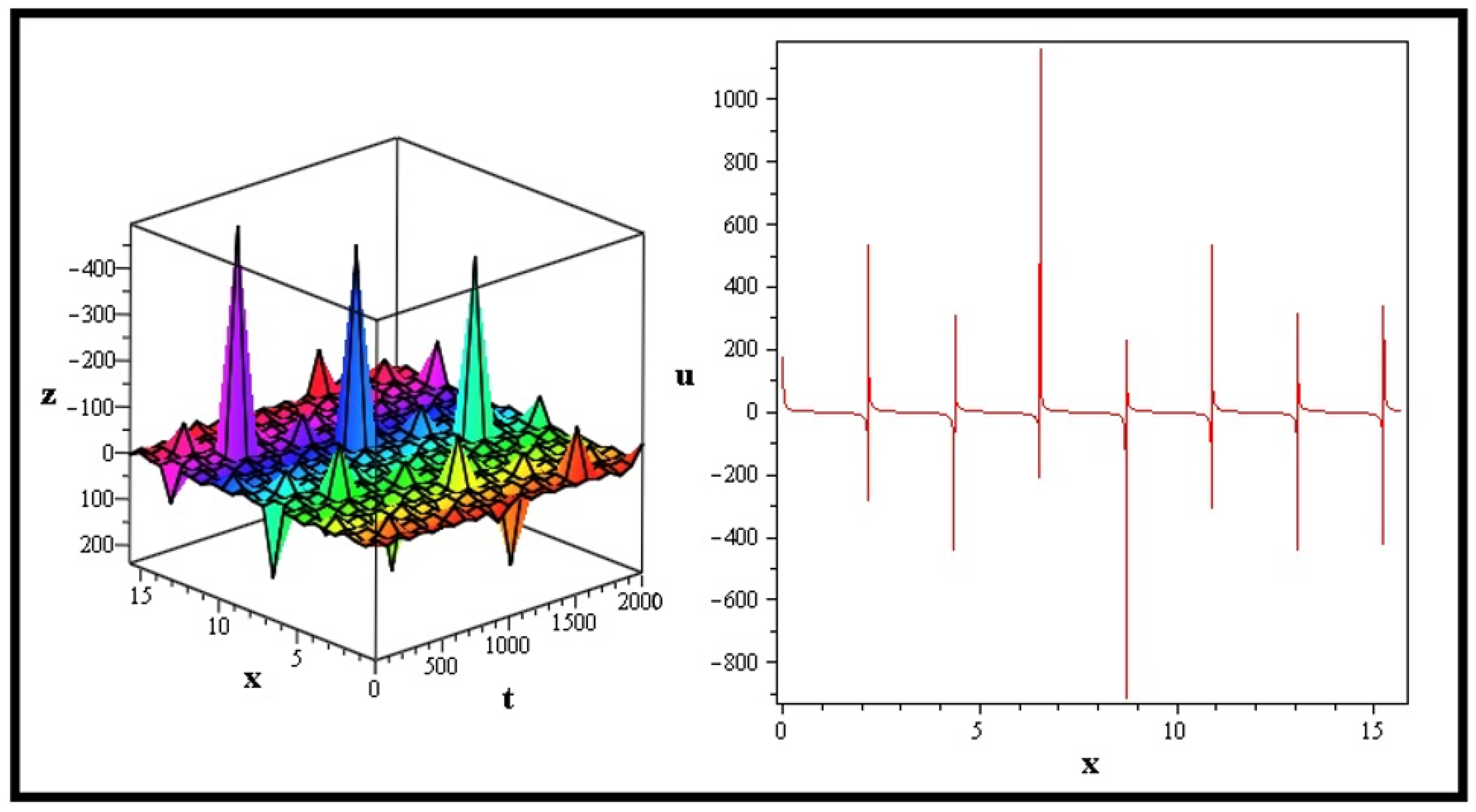
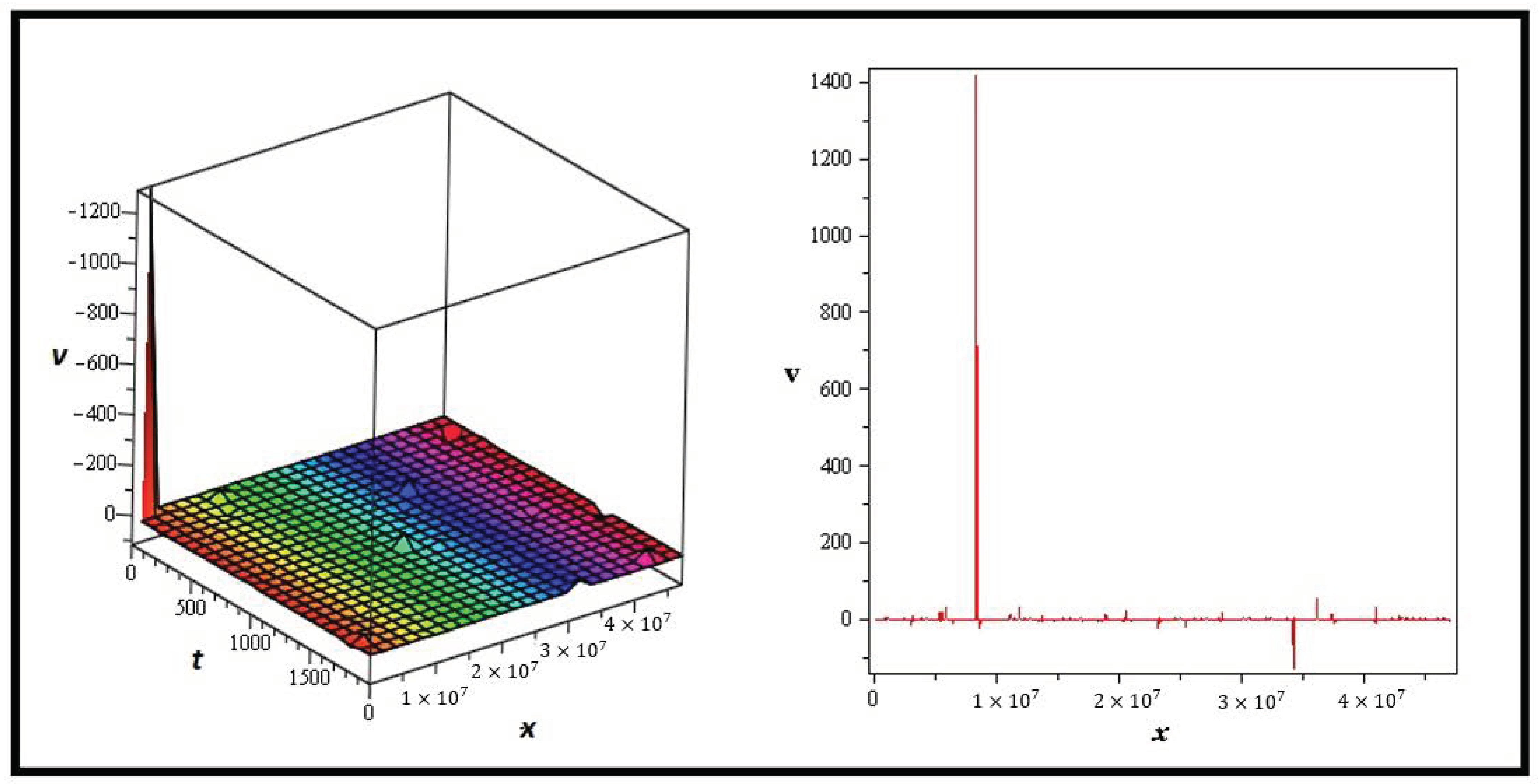
4. Discussion and Graphs

In this article, we investigated families of soliton solutions for the complex structured coupled FBAM in Birefringent Fibers using a unique analytical method termed mEDAM. Using this method, we were able to transform the supplied set of nonlinear ODEs derived from the model into a set of algebraic equations by supposing a series form solution. We were able to obtain the soliton solutions for the model by resolving these equations. The CFBAM in Birefringent Fibers’ soliton solutions developed by the mEDAM approach have important physical implications and provide profound insights into the fundamental processes of the model. These solutions make it easier to investigate how various model parameters impact soliton dynamics, since they have unique characteristics including amplitude, width, and propagation speed. They also aid in understanding the nonlinear dispersion and self-steepening effects of the model, which influence the soliton profiles and control their propagation behavior. Overall, these findings advance our understanding of the subject matter and provide direction for more research and application in the area.

The resulting soliton solutions include a variety of traveling wave solutions, including periodic, lump, kink, and rogue waves. The fact that these waves may be represented by the governing equations of the FBAM in birefringent fibers indicates the connection between these waves and the model. Birefringent fibers, which have two distinct refractive indices along two orthogonal axes, are used in the model to represent how light waves move through them. The Kerr effect, which causes the refractive index to change with the strength of the light wave, is the cause of the nonlinearities in the model. The non-local and memory effects are taken into consideration by the inclusion of the fractional derivative in the model.

Remark 1.

Figure 1 depicts a lone rogue wave, an unusual and dangerous maritime phenomena marked by its sudden and unnaturally large amplitude. Due to their reputation for unpredictable and destructive activity, rogue waves are a topic of interest in a variety of research fields. The possibility that such odd events may occur during the propagation of light waves in these fibers makes the discovery of rogue waves in the FBAM’s soliton solutions in birefringent fibers intriguing. Understanding the behavior of rogue waves in this scenario will help in the development of more reliable and robust fiber-optic communication systems and sensors.

Remark 2.

Figure 2 depicts a periodic wave’s profile as well as the repeating nature of periodic oscillations throughout time. Periodic waves can be seen in the soliton solutions of the FBAM in birefringent fibers due to the inclusion of nonlinear processes that could cause modulational instability and self-phase modulation. The periodic wave solutions that might be created as a result of these effects can be seen in the soliton solutions discovered utilizing the mEDAM technique.

Remark 3.

Figure 3 displays the profile of a lump wave in our soliton solutions for the FBAM in birefringent fibers. As significant solutions, lump waves can show themselves in a number of physical systems. They are distinguished by a sharp amplitude surge and a gradual fall back to the initial level. Our soliton solutions contain lump waves, indicating that they have an impact on how light waves behave in birefringent fibers and may be crucial for the development of fiber-optic communication systems and sensors.

Remark 4.

Figure 4 depicts the profile of a kink wave, a specific wave type identified by an abrupt change in direction or a sharp bend. These waves are present in our soliton solutions for the FBAM in birefringent fibers. Kink waves are crucial to fiber-optic communication systems because they may be utilized to regulate how light waves travel through birefringent fibers. Our soliton solutions demonstrate how the kink wave may be used to enhance fiber-optic communication systems’ performance by better regulating light wave propagation.

5. Conclusions

The complex structured coupled FBAM in Birefringent Fibers was studied using a unique analytical method known as the mEDAM. For the provided system of nonlinear ODEs derived from the model, the mEDAM approach was able to find a series form closed solution, which was then transformed into a set of algebraic equations to find soliton solutions for the model. Different varieties of traveling wave solutions that are important to the model’s physical interpretation can be found in the derived soliton solutions. The presence of various traveling wave solutions, including kink, rogue, lump, and periodic waves, in soliton solutions was illustrated visually by displaying some 2D and 3D graphs. These waves can help in the creation of cutting-edge fiber-optic communication systems and sensors by shedding light on how light waves behave in birefringent fibers. The article focuses on the implications for various real-world optical applications and shows how the mEDAM technique may be used to analyze families of traveling soliton solutions for complicated models.

References

1. Zayed, E.M.; Amer, Y.A.; Shohib, R.M. The fractional complex transformation for nonlinear fractional partial differential equations in the mathematical physics. J. Assoc. Arab. Univ. Basic Appl. Sci. 2016, 19, 59–69. [Google Scholar] [CrossRef] [Green Version]
2. Sun, H.; Zhang, Y.; Baleanu, D.; Chen, W.; Chen, Y. A new collection of real world applications of fractional calculus in science and engineering. Commun. Nonlinear Sci. Numer. Simul. 2018, 64, 213–231. [Google Scholar] [CrossRef]
3. Singh, J.; Kumar, D.; Kılıçman, A. Numerical solutions of nonlinear fractional partial differential equations arising in spatial diffusion of biological populations. Abstr. Appl. Anal. 2014, 2014, 535793. [Google Scholar] [CrossRef] [Green Version]
4. Ara, A.; Khan, N.A.; Razzaq, O.A.; Hameed, T.; Raja, M.A.Z. Wavelets optimization method for evaluation of fractional partial differential equations: An application to financial modelling. Adv. Differ. Equ. 2018, 2018, 8. [Google Scholar] [CrossRef]
5. Pan, S.; Lin, M.; Xu, M.; Zhu, S.; Bian, L.; Li, G. A Low-Profile Programmable Beam Scanning Holographic Array Antenna Without Phase Shifters. IEEE Internet Things J. 2022, 9, 8838–8851. [Google Scholar] [CrossRef]
6. Zhao, C.; Cheung, C.F.; Xu, P. High-efficiency sub-microscale uncertainty measurement method using pattern recognition. ISA Trans. 2020, 101, 503–514. [Google Scholar] [CrossRef]
7. Jin, H.Y.; Wang, Z.A. Global stabilization of the full attraction-repulsion Keller-Segel system. Discret. Contin. Dyn. Syst.-Ser. A 2020, 40, 3509–3527. [Google Scholar] [CrossRef] [Green Version]
8. Lyu, W.; Wang, Z. Global classical solutions for a class of reaction-diffusion system with density-suppressed motility. Electron. Res. Arch. 2022, 30, 995–1015. [Google Scholar] [CrossRef]
9. Zhang, J.; Xie, J.; Shi, W.; Huo, Y.; Ren, Z.; He, D. Resonance and bifurcation of fractional quintic Mathieu–Duffing system. Chaos Interdiscip. J. Nonlinear Sci. 2023, 33, 23131. [Google Scholar] [CrossRef]
10. El-Sheikh, M.M.A.; Ahmed, H.M.; Arnous, A.H.; Rabie, W.B. Optical solitons and other solutions in birefringent fibers with Biswas–Arshed equation by Jacobi’s elliptic function approach. Optik 2020, 202, 163546. [Google Scholar] [CrossRef]
11. Pandir, Y.; Ekin, A. New solitary wave solutions of the Korteweg-de Vries (KdV) equation by new version of the trial equation method. Electron. J. Appl. Math. 2023, 1, 101–113. [Google Scholar]
12. Meerschaert, M.M.; Tadjeran, C. Finite difference approximations for two-sided space-fractional partial differential equations. Appl. Numer. Math. 2006, 56, 80–90. [Google Scholar] [CrossRef]
13. Zhang, H.; Liu, F.; Anh, V. Galerkin finite element approximation of symmetric space-fractional partial differential equations. Appl. Math. Comput. 2010, 217, 2534–2545. [Google Scholar] [CrossRef]
14. Wu, J.L. A wavelet operational method for solving fractional partial differential equations numerically. Appl. Math. Comput. 2009, 214, 31–40. [Google Scholar] [CrossRef]
15. Momani, S.; Odibat, Z. A novel method for nonlinear fractional partial differential equations: Combination of DTM and generalized Taylor’s formula. J. Comput. Appl. Math. 2008, 220, 85–95. [Google Scholar] [CrossRef]
16. Ziane, D.; Cherif, M.H. Variational iteration transform method for fractional differential equations. J. Interdiscip. Math. 2018, 21, 185–199. [Google Scholar] [CrossRef]
17. Khan, H.; Baleanu, D.; Kumam, P.; Al-Zaidy, J.F. Families of travelling waves solutions for fractional-order extended shallow water wave equations, using an innovative analytical method. IEEE Access 2019, 7, 107523–107532. [Google Scholar] [CrossRef]
18. Manafian, J.; Foroutan, M. Application of tan(ϕ(ξ)/2)-expansion method for the time-fractional Kuramoto–Sivashinsky equation. Opt. Quantum Electron. 2017, 49, 272. [Google Scholar] [CrossRef]
19. Zheng, B. Exp-function method for solving fractional partial differential equations. Sci. World J. 2013, 2013, 465723. [Google Scholar] [CrossRef] [PubMed] [Green Version]
20. Younis, M.; Iftikhar, M. Computational examples of a class of fractional order nonlinear evolution equations using modified extended direct algebraic method. J. Comput. Methods Sci. Eng. 2015, 15, 359–365. [Google Scholar] [CrossRef]
21. Qi, M.; Cui, S.; Chang, X.; Xu, Y.; Meng, H.; Wang, Y.; Arif, M. Multi-region Nonuniform Brightness Correction Algorithm Based on L-Channel Gamma Transform. Secur. Commun. Netw. 2022, 2022, 2675950. [Google Scholar] [CrossRef]
22. Guo, F.; Zhou, W.; Lu, Q.; Zhang, C. Path extension similarity link prediction method based on matrix algebra in directed networks. Comput. Commun. 2022, 187, 83–92. [Google Scholar] [CrossRef]
23. Song, J.; Mingotti, A.; Zhang, J.; Peretto, L.; Wen, H. Accurate Damping Factor and Frequency Estimation for Damped Real-Valued Sinusoidal Signals. IEEE Trans. Instrum. Meas. 2022, 71, 6503504. [Google Scholar] [CrossRef]
24. Liu, H.; Li, J.; Meng, X.; Zhou, B.; Fang, G.; Spencer, B.F. Discrimination between Dry and Water Ices by Full Polarimetric Radar: Implications for China’s First Martian Exploration. IEEE Trans. Geosci. Remote. Sens. 2022, 61, 5100111. [Google Scholar] [CrossRef]
25. Fu, Q.; Si, L.; Liu, J.; Shi, H.; Li, Y. Design and experimental study of a polarization imaging optical system for oil spills on sea surfaces. Appl. Opt. 2022, 61, 6330–6338. [Google Scholar] [CrossRef] [PubMed]
26. Li, Z. Bifurcation and traveling wave solution to fractional Biswas–Arshed equation with the beta time derivative. Chaos Solitons Fractals 2022, 160, 112249. [Google Scholar] [CrossRef]
27. Ozkan, Y.S. On the exact solutions to Biswas–Arshed equation involving truncated M-fractional space-time derivative terms. Optik 2021, 227, 166109. [Google Scholar] [CrossRef]
28. Zafar, A.; Bekir, A.; Raheel, M.; Razzaq, W. Optical soliton solutions to Biswas–Arshed model with truncated M-fractional derivative. Optik 2020, 222, 165355. [Google Scholar] [CrossRef]
29. Hosseini, K.; Mirzazadeh, M.; Ilie, M.; Gomez-Aguilar, J.F. Biswas–Arshed equation with the beta time derivative: Optical solitons and other solutions. Optik 2020, 217, 164801. [Google Scholar] [CrossRef]
30. Demiray, S.T. New solutions of Biswas–Arshed equation with beta time derivative. Optik 2020, 222, 165405. [Google Scholar] [CrossRef]
31. Naeem, M.; Yasmin, H.; Shah, R.; Shah, N.A.; Chung, J.D. A Comparative Study of Fractional Partial Differential Equations with the Help of Yang Transform. Symmetry 2023, 15, 146. [Google Scholar] [CrossRef]
32. Mirhosseini-Alizamini, S.M.; Rezazadeh, H.; Srinivasa, K.; Bekir, A. New closed form solutions of the new coupled Konno-Oono equation using the new extended direct algebraic method. Pramana 2020, 94, 52. [Google Scholar] [CrossRef]
Figure 1. The first equation in (44) is displayed with a three-dimensional graph for a = 10.64 , b = 0 , c = 0.19 , A = 2 , h 1 = 1 , h 2 = 2 , h 3 = 109 , ω = 0 , ν = 2 , α = β = 1 , while the 2D graph is plotted by assuming t = 0 and for the same values of parameters involved.
Fractalfract 07 00491 g001
Figure 2. The first equation in (45) is displayed with a three-dimensional graph for a = 10.64 , b = 0 , c = 0.19 , p = 5 , q = 2 , A = 2 , h 1 = 1 , h 2 = 2 , h 3 = 109 , ω = 0 , ν = 2 , α = β = 1 , while the 2D graph is plotted by assuming t = 0 and for the same values of parameters involved.
Fractalfract 07 00491 g002
Figure 3. The first equation in (66) is displayed with a three-dimensional graph for a = 10.64 , b = 0 , c = 0 , A = 2 , h 1 = 1 , h 2 = 2 , h 3 = 109 , ω = 0 , ν = 2 , α = β = 1 , while the 2D graph is plotted by assuming t = 2 and for the same values of parameters involved.
Fractalfract 07 00491 g003
Figure 4. The first equation in (80) is displayed with a three-dimensional graph for b = 10.64 , b = 0 , a = 0.19 , A = 2 , h 1 = 1 , h 2 = 2 , h 3 = 109 , ω = 0 , ν = 2 , α = 0.2 , β = 0.9 , while the 2D graph is plotted by assuming t = 2 and for the same values of parameters involved.
Fractalfract 07 00491 g004
Disclaimer/Publisher’s Note: The statements, opinions and data contained in all publications are solely those of the individual author(s) and contributor(s) and not of MDPI and/or the editor(s). MDPI and/or the editor(s) disclaim responsibility for any injury to people or property resulting from any ideas, methods, instructions or products referred to in the content.