
Synchronization of Discrete-Time Fractional-Order Complex-Valued Neural Networks with Distributed Delays
 , , and
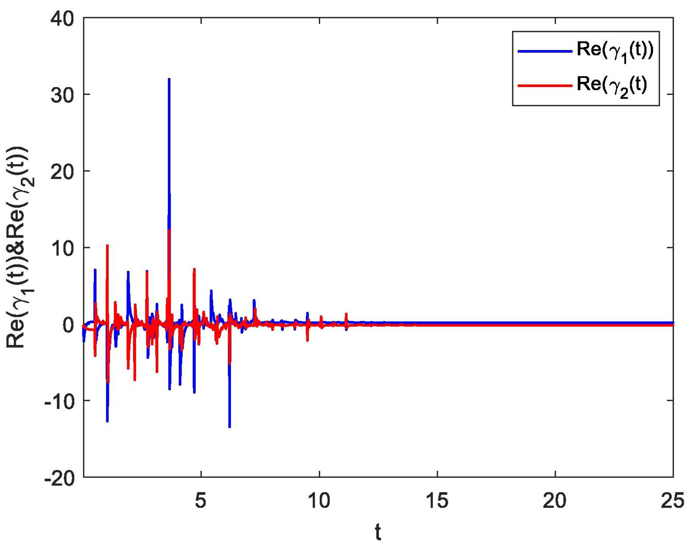
Abstract
:1. Introduction
- (1)
- We studied the global synchronization of discrete-time fractional-order complex-valued neural networks with distributed delays.
- (2)
- Unlike the previous literature, this paper explicitly examines the stability for discrete fractional-order complex-valued neural networks using the stability theory in complex fields as opposed to breaking down complex-valued systems into real-valued systems.
- (3)
- Using the Lyapunov direct technique, the synchronization condition of FOCVNNs with temporal delays is determined. In light of the definition of the Caputo fractional difference, it is simple to calculate the first-order backward difference of the Lyapunov function that we design, which includes discrete fractional sum terms.
- (4)
- Some conditions regarding the global Mittag-Leffler stability of fractional-order CVNNs are established using fractional derivative inequalities and fractional-order appropriate Lyapunov functions.
- (5)
- It is necessary to investigate the essential characteristics of the discrete Mittag–Leffler function and the Nabla discrete Laplace transform.
- (6)
- Finally, numerical illustrations are provided.
2. Preliminaries
3. Main Results
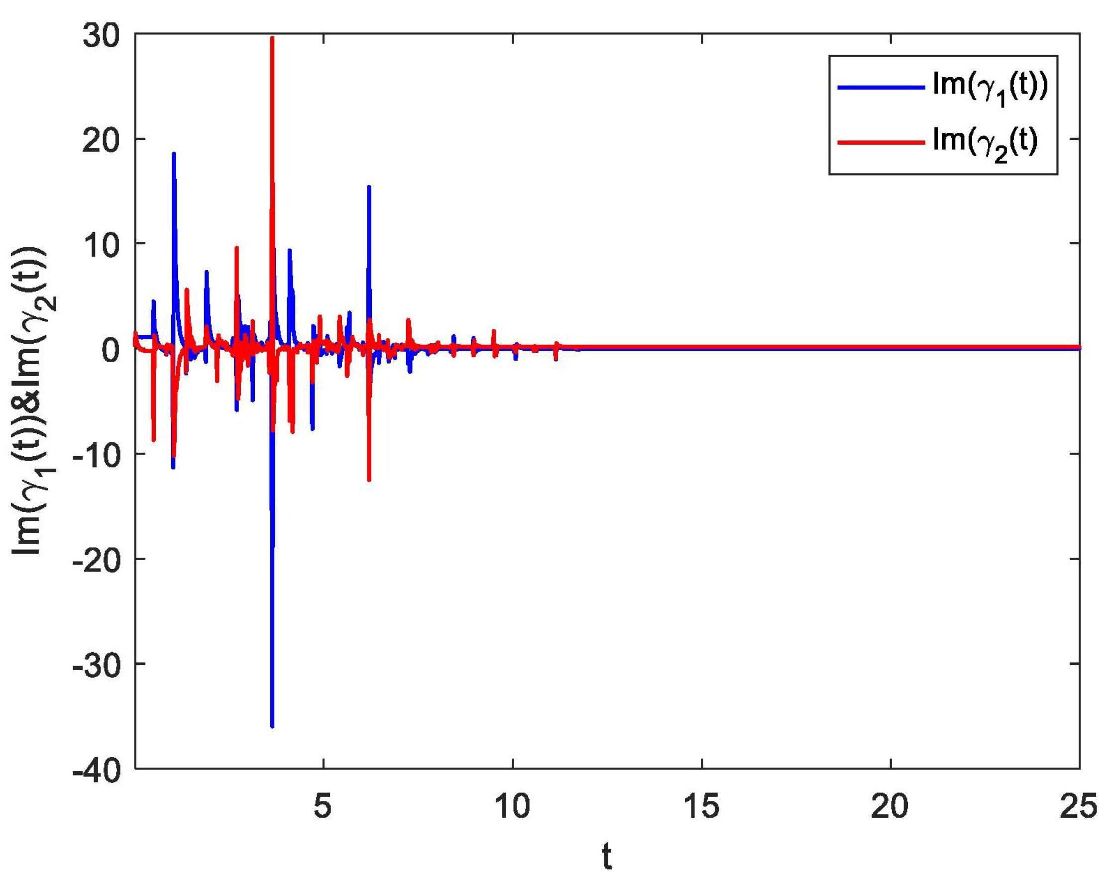
4. Numerical Examples
5. Conclusions
Author Contributions
Funding
Data Availability Statement
Acknowledgments
Conflicts of Interest
References
- Ahmeda, E.; Elgazzar, A. On fractional order differential equations model for nonlocal epidemics. Physica A 2007, 379, 607–614. [Google Scholar] [CrossRef] [PubMed]
- Moaddy, K.; Radwan, A.; Salama, K.; Momani, S.; Hashim, I. The fractional-order modeling and synchronization of electrically coupled neuron systems. Comput. Math. Appl. 2012, 64, 3329–3339. [Google Scholar] [CrossRef]
- Bhalekar, S.; Daftardar-Gejji, V. Synchronization of differential fractional-order chaotic systems using active control. Commun. Nonlinear Sci. Numer. Simul. 2010, 15, 3536–3546. [Google Scholar] [CrossRef]
- Narayanan, G.; Ali, M.S.; Karthikeyan, R.; Rajchakit, G.; Jirawattanapanit, A. Impulsive control strategies of mRNA and protein dynamics on fractional-order genetic regulatory networks with actuator saturation and its oscillations in repressilator model. Biomed. Process. Control 2023, 82, 104576. [Google Scholar] [CrossRef]
- Jmal, A.; Makhlouf, A.B.; Nagy, A.M. Finite-Time Stability for Caputo Katugampola Fractional-Order Time-Delayed Neural Networks. Neural Process Lett. 2019, 50, 607–621. [Google Scholar] [CrossRef]
- Li, H.L.; Jiang, H.; Cao, J. Global synchronization of fractional-order quaternion-valued neural networks with leakage and discrete delays. Neurocomputing 2020, 385, 211–219. [Google Scholar] [CrossRef]
- Chen, S.; An, Q.; Ye, Y.; Su, H. Positive consensus of fractional-order multi-agent systems. Neural Comput. Appl. 2021, 33, 16139–16148. [Google Scholar] [CrossRef]
- Chen, S.; An, Q.; Zhou, H.; Su, H. Observer-based consensus for fractional-order multi-agent systems with positive constraint Author links open overlay panel. Neurocomputing 2022, 501, 489–498. [Google Scholar] [CrossRef]
- Li, Z.Y.; Wei, Y.H.; Wang, J.; Li, A.; Wang, J.; Wang, Y. Fractional-order ADRC framework for fractional-order parallel systems. In Proceedings of the 2020 39th Chinese Control Conference (CCC), Shenyang, China, 27–29 July 2020; pp. 1813–1818. [Google Scholar]
- Wang, L. Symmetry and conserved quantities of Hamilton system with comfortable fractional derivatives. In Proceedings of the 2020 Chinese Control And Decision Conference (CCDC), Hefei, China, 22–24 August 2020; pp. 3430–3436. [Google Scholar]
- Castañeda, C.E.; López-Mancilla, D.; Chiu, R.; Villafana-Rauda, E.; Orozco-López, O.; Casillas-Rodríguez, F.; Sevilla-Escoboza, R. Discrete-time neural synchronization between an arduino microcontroller and a compact development system using multiscroll chaotic signals. Chaos Solitons Fractals 2019, 119, 269–275. [Google Scholar] [CrossRef]
- Atici, F.M.; Eloe, P.W. Gronwalls inequality on discrete fractional calculus. Comput. Math. Appl. 2012, 64, 3193–3200. [Google Scholar] [CrossRef]
- Ostalczyk, P. Discrete Fractional Calculus: Applications in Control and Image Processing; World Scientific: Singapore, 2015. [Google Scholar]
- Ganji, M.; Gharari, F. The discrete delta and nabla Mittag-Leffler distributions. Commun. Stat. Theory Methods 2018, 47, 4568–4589. [Google Scholar] [CrossRef]
- Wyrwas, M.; Mozyrska, D.; Girejko, E. Stability of discrete fractional-order nonlinear systems with the nabla Caputo difference. IFAC Proc. Vol. 2013, 46, 167–171. [Google Scholar] [CrossRef]
- Gray, H.L.; Zhang, N.F. On a new definition of the fractional difference. Math. Comput. 1988, 50, 513–529. [Google Scholar] [CrossRef]
- Wu, G.C.; Baleanu, D.; Luo, W.H. Lyapunov functions for Riemann-Liouville-like fractional difference equations. Appl. Math. Comput. 2017, 314, 228–236. [Google Scholar] [CrossRef]
- Baleanu, D.; Wu, G.C.; Bai, Y.R.; Chen, F.L. Stability analysis of Caputolike discrete fractional systems. Commun. Nonlinear Sci. Numer. Simul. 2017, 48, 520–530. [Google Scholar] [CrossRef]
- Hu, J.; Wang, J. Global stability of complex-valued recurrent neural networks with time-delays. IEEE Trans. Neural Netw. Learn. Syst. 2012, 23, 853–865. [Google Scholar] [CrossRef] [PubMed]
- Ozdemir, N.; Iskender, B.B.; Ozgur, N.Y. Complex valued neural network with Mobius activation function. Commun. Nonlinear Sci. Numer. Simul. 2011, 16, 4698–4703. [Google Scholar] [CrossRef]
- Rakkiyappan, R.; Cao, J.; Velmurugan, G. Existence and uniform stability analysis of fractional-order complex-valued neural networks with time delays. IEEE Trans. Neural Netw. Learn. Syst. 2015, 26, 84–97. [Google Scholar] [CrossRef]
- Song, Q.; Zhao, Z.; Liu, Y. Stability analysis of complex-valued neural networks with probabilistic time-varying delays. Neurocomputing 2015, 159, 96–104. [Google Scholar] [CrossRef]
- Pan, J.; Liu, X.; Xie, W. Exponential stability of a class of complex-valued neural networks with time-varying delays. Neurocomputing 2015, 164, 293–299. [Google Scholar] [CrossRef]
- Li, X.; Rakkiyappan, R.; Velmurugan, G. Dissipativity analysis of memristor-based complex-valued neural networks with time-varying delays. Inf. Sci. 2015, 294, 645–665. [Google Scholar] [CrossRef]
- Rakkiyappan, R.; Sivaranjani, K.; Velmurugan, G. Passivity and passification of memristor-based complex-valued recurrent neural networks with interval time-varying delays. Neurocomputing 2014, 144, 391–407. [Google Scholar] [CrossRef]
- Chen, L.P.; Chai, Y.; Wu, R.C.; Ma, T.D.; Zhai, H.Z. Dynamic analysis of a class of fractional-order neural networks with delay. Neurocomputing 2013, 111, 190–194. [Google Scholar] [CrossRef]
- Song, Q.; Yan, H.; Zhao, Z.; Liu, Y. Global exponential stability of complex-valued neural networks with both time-varying delays and impulsive effects. Neural Netw. 2016, 79, 108–116. [Google Scholar] [CrossRef]
- Syed Ali, M.; Yogambigai, J.; Kwon, O.M. Finite-time robust passive control for a class of switched reaction-diffusion stochastic complex dynamical networks with coupling delays and impulsive control. Int. J. Syst. Sci. 2018, 49, 718–735. [Google Scholar] [CrossRef]
- Zhou, B.; Song, Q. Boundedness and complete stability of complex valued neural networks with time delay. IEEE Trans. Neural Netw. Learn. Syst. 2013, 24, 1227–1238. [Google Scholar] [CrossRef]
- Zhang, Z.; Lin, C.; Chen, B. Global stability criterion for delayed complex-valued recurrent neural networks. IEEE Trans. Neural Netw. Learn. Syst. 2014, 25, 1704–1708. [Google Scholar] [CrossRef]
- Song, Q.; Zhao, Z. Stability criterion of complex-valued neural networks with both leakage delay and time-varying delays on time scales. Neurocomputing 2016, 171, 179–184. [Google Scholar] [CrossRef]
- Sakthivel, R.; Sakthivel, R.; Kwon, O.M.; Selvaraj, P.; Anthoni, S.M. Observer-based robust synchronization of fractional-order multi-weighted complex dynamical networks. Nonlinear Dyn. 2019, 98, 1231–1246. [Google Scholar] [CrossRef]
- Chen, X.; Song, Q. Global stability of complex-valued neural networks with both leakage time delay and discrete time delay on time scales. Neurocomputing 2013, 121, 254–264. [Google Scholar] [CrossRef]
- Zhang, Z.; Yu, S. Global asymptotic stability for a class of complex valued Cohen-Grossberg neural networks with time delays. Neurocomputing 2016, 171, 1158–1166. [Google Scholar] [CrossRef]
- Gong, W.; Liang, J.; Cao, J. Matrix measure method for global exponential stability of complex-valued recurrent neural networks with time-varying delays. Neural Netw. 2015, 70, 81–89. [Google Scholar] [CrossRef]
- Syed Ali, M.; Yogambigai, J.; Cao, J. Synchronization of master-slave Markovian switching complex dynamical networks with time-varying delays in nonlinear function via sliding mode control. Acta Math. Sci. 2017, 37, 368–384. [Google Scholar]
- Zhou, J.; Liu, Y.; Xia, J.; Wang, Z.; Arik, S. Resilient fault-tolerant antisynchronization for stochastic delayed reaction-diffusion neural networks with semi-Markov jump parameters. Neural Netw. 2020, 125, 194–204. [Google Scholar] [CrossRef] [PubMed]
- Syed Ali, M.; Yogambigai, J. Finite-time robust stochastic synchronization of uncertain Markovian complex dynamical networks with mixed time-varying delays and reaction-diffusion terms via impulsive control. J. Frankl. Inst. 2017, 354, 2415–2436. [Google Scholar]
- Narayanan, G.; Syed Ali, M.; Karthikeyan, R.; Rajchakit, G.; Jirawattanapanit, A. Novel adaptive strategies for synchronization mechanism in nonlinear dynamic fuzzy modeling of fractional-order genetic regulatory networks. Chaos Solitons Fractals 2022, 165, 112748. [Google Scholar] [CrossRef]
- Yogambigai, J.; Syed Ali, M. Exponential Synchronization of switched complex dynamical networks with time varying delay via periodically intermittent control. Int. J. Differ. Equ. 2017, 12, 41–53. [Google Scholar]
- Yogambigai, J.; Syed Ali, M. Finite-time and Sampled-data Synchronization of Delayed Markovian Jump Complex Dynamical Networks Based on Passive Theory. In Proceedings of the Third International Conference on Science Technology Engineering and Management (ICONSTEM), Chennai, India, 23–24 March 2017. [Google Scholar]
- Yang, L.X.; Jiang, J. Adaptive synchronization of driveresponse fractional-order complex dynamical networks with uncertain parameters. Commun. Nonlinear Sci. Numer. Simul. 2014, 19, 1496–1506. [Google Scholar] [CrossRef]
- Wong, W.K.; Li, H.; Leung, S.Y.S. Robust synchronization of fractional-order complex dynamical networks with parametric uncertainties. Commun. Nonlinear Sci. Numer. Simul. 2012, 17, 4877–4890. [Google Scholar] [CrossRef]
- Bao, H.; Park, J.H.; Cao, J. Synchronization of fractional order complex-valued neural networks with time delay. Neural Netw. 2016, 81, 16–28. [Google Scholar] [CrossRef]
- Qi, D.L.; Liu, M.Q.; Qiu, M.K.; Zhang, S.L. Exponential H∞ synchronization of general discrete-time chaotic neural networks with or without time delays. IEEE Trans. Neural Netw. Learn. Syst. 2010, 21, 1358–1365. [Google Scholar]
- Li, Z.Y.; Liu, H.; Lu, J.A.; Zeng, Z.G.; Lü, J. Synchronization regions of discrete-time dynamical networks with impulsive couplings. Inf. Sci. 2018, 459, 265–277. [Google Scholar] [CrossRef]
- You, X.; Song, Q.; Zhao, Z. Global Mittag-Leffler stability and synchronization of discrete-time fractional-order complex-valued neural networks with time delay. Neural Netw. 2020, 122, 382–394. [Google Scholar] [CrossRef]
- Atici, F.M.; Eloe, P.W. Discrete fractional calculus with the nabla operator. Electron. J. Qual. Theory Differ. Equ. 2009, 3, 1–12. [Google Scholar] [CrossRef]
- Mu, X.X.; Chen, Y.G. Synchronization of delayed discrete-time neural networks subject to saturated time-delay feedback. Neurocomputing 2016, 175, 293–299. [Google Scholar] [CrossRef]
- Liang, S.; Wu, R.C.; Chen, L.P. Comparison principles and stability of nonlinear fractional-order cellular neural networks with multiple time delays. Neurocomputing 2015, 168, 618–625. [Google Scholar] [CrossRef]


Disclaimer/Publisher’s Note: The statements, opinions and data contained in all publications are solely those of the individual author(s) and contributor(s) and not of MDPI and/or the editor(s). MDPI and/or the editor(s) disclaim responsibility for any injury to people or property resulting from any ideas, methods, instructions or products referred to in the content. |
© 2023 by the authors. Licensee MDPI, Basel, Switzerland. This article is an open access article distributed under the terms and conditions of the Creative Commons Attribution (CC BY) license (https://creativecommons.org/licenses/by/4.0/).
Share and Cite
Perumal, R.; Hymavathi, M.; Ali, M.S.; Mahmoud, B.A.A.; Osman, W.M.; Ibrahim, T.F. Synchronization of Discrete-Time Fractional-Order Complex-Valued Neural Networks with Distributed Delays. Fractal Fract. 2023, 7, 452. https://doi.org/10.3390/fractalfract7060452
Perumal R, Hymavathi M, Ali MS, Mahmoud BAA, Osman WM, Ibrahim TF. Synchronization of Discrete-Time Fractional-Order Complex-Valued Neural Networks with Distributed Delays. Fractal and Fractional. 2023; 7(6):452. https://doi.org/10.3390/fractalfract7060452
Chicago/Turabian StylePerumal, R., M. Hymavathi, M. Syed Ali, Batul A. A. Mahmoud, Waleed M. Osman, and Tarek F. Ibrahim. 2023. "Synchronization of Discrete-Time Fractional-Order Complex-Valued Neural Networks with Distributed Delays" Fractal and Fractional 7, no. 6: 452. https://doi.org/10.3390/fractalfract7060452