1. Introduction
The aim of this research was to ensure the repeatability of fractal analysis results of non-orthogonal representations of architecture in street-space, be it in the form of photographs or CAD-generated, 3D model-based imagery. This was formulated as a method that uses 360-degree spherical panoramas as a basis for fractal measurement, which is called spherical perspective box-counting. From here on, it is also referred to as spherical box-counting. It is demonstrated as an exemplary implementation in the web-based platform FRACAM (“Fractal Camera”) [
1], and it was tested on six CAD-generated pictures based on a parametric 3D model and thirteen spherical photographs depicting five exterior and two interior spaces (see
Section 3, Results).
Based on the hypothesis that architectural quality and architectural characteristics can be linked to fractal characteristics, such as roughness, complexity, self-similarity, and scale-invariance, not least by aesthetic rules connected to fractal theory [
2,
3,
4,
5,
6,
7,
8], this paper describes an extended fractal measurement method for evaluating the complexity of architecture using 360-degree spherical images. This method improves several aspects of the quantitative evaluation of buildings—primarily represented as façades in the street space—by employing box-counting. The influence of the correct placement of the measurement grid over the representation of the elevation is thereby minimized (which was previously achieved using white border and grid displacement), which is necessary to find the minimum number of covering boxes [
9,
10,
11]—see
Section 2.1.1 for more information. Moreover, the spherical box-counting method proposed here takes into account the perspective non-orthogonal perception of the street space (see [
12]) at the same time, eliminating the influence of a deliberate choice of one specific image section.
360 degree spherical images provide an all-around view from a chosen location. Buildings are not solely measured as isolated objects, but by taking their environment, be it natural or man-made, into account.
The analysis is viewer-location specific for both photograph and model analysis; if photographs are used, then the values of the analysis are subject to influence by time of day, season, and weather conditions (recently mentioned in [
13]). Analyses that do not take perspective respective to viewer location—i.e., an approximation to actual observation—into account do not have these limitations. However, they do have the weakness of focusing on an idea about architecture as geometry and not the appearance of built architecture; the central problem of abstract and actual architecture representation was discussed by Vaughan and Ostwald [
14]. To address the problems connected to fractal analysis of architecture as appearance, FRACAM was developed [
1]; the spherical box-counting process on the basis of photographs builds on this research.
The described method does enhance FRACAM but is not limited to implementation in this software. It represents a general approach that eliminates the problem of deliberately choosing a picture frame when dealing with vanishing point perspective imagery as a basis for fractal analysis methods. The implementation of this method in the existing web application FRACAM as an enhancement is exemplary.
As shown in
Section 2.2, Spherical Representation, spherical box-counting can be applied to CAD models as a controlled environment, ensuring the repeatability of calculations and their resulting values. Using computer-generated imagery based on 3D models allows for including, e.g., time of day, season, and weather conditions and the like in a controlled fashion. These aspects may be left aside to pinpoint specific layers of analysis separately while preserving observer location-based representation.
1.1. Aesthetic Qualities, Fractal Geometry, and Architecture
Architecture is not least the pursuit of an aesthetic quality. In order to describe and reach such an aesthetic quality, architects, designers, and mathematicians have developed various theories that are considered valid due to centuries of application. These theories include proportion theory as well as color theory (e.g., [
15,
16,
17,
18,
19]). They imply that if a designer follows certain rules, e.g., the golden section as a system of measurement proportions to relate whole form to detail, this may lead to a certain quality that links it to other (possibly iconic) buildings. Although it is very likely impossible to objectify successful aesthetic quality in its entirety, it is a sensible goal to conceive and improve measuring methods that provide significant aid in developing aesthetic quality and making valuable judgments about it on the grounds of complexity after materialization. It can be shown that the box-counting method, originating from fractal theory, is one of these methods that can make aesthetic quality more tangible (see [
5,
12,
13]).
1.2. Architecture and Fractals
The word “fractal” is a term coined by Benoit Mandelbrot in the year 1975 [
20] to describe irregular, non-smooth curves. It also addresses phenomena and complex objects difficult to capture using traditional terms, including fractal shapes of mountains and snowflakes, fractal fluctuations in the healthy human heartbeat, fractal growth of cities, medical diagnoses of, e.g., cancer, but also applications such as fractal image compression [
3,
9,
21,
22,
23,
24]. “Fractal” stems from the Latin verb “frangere” meaning “to break into irregular fragments” and being “rugged” or “rough” in some fashion, which points to a central property of fractals [
25]. Other attributes include (statistical) self-similarity, i.e., parts resembling the whole, infinite complexity albeit describable with simple algorithms, generation through iterations (meaning a transformation is applied to itself over and over again), and a fractal dimension that exceeds the topological dimension [
3,
21]. Although the literature does not provide one precise definition of fractals (see [
26,
27,
28]), they appear to be closer to nature and share the attribute of irregularity that repeats itself geometrically across many scales [
21]. The latter is connected to human perception and pattern recognition as described in cognitive sciences. Again and again, we find (statistically) self-similar (at least in a certain range of scales), rough, and to some extent, complex objects that follow a simpler basic description in their formation.
The phenomena studied by Mandelbrot can only be described with difficulty using the Euclidean geometry that we are familiar with, an aspect that is underscored by the quotation, “
Clouds are not spheres, mountains are not cones, coastlines are not circles, and bark is not smooth” [
3]. Therefore, he introduced what he called fractal geometry. If we take a closer look at architecture, and in particular façades, it becomes obvious that some of the properties that describe fractals also apply here. Accordingly, a “Gründerzeit” façade is not smooth, but rather rough, and it is caused by cornices and other architectural details (not least by openings such as windows and doors). “Gründerzeit” is a term used primarily in Austria for the period between 1840 and 1918 in which buildings were erected in the style of historicism “from the catalogue”. Moreover, gothic cathedrals are good examples for fractal-like architecture in which the whole and its parts are held together by a basic theme, the pursuit of heaven. These examples show architectural elements that suit different distances from the viewer, i.e., there is always something to see on the right (human) scale [
7].
When it is stated that fractals are very complex, this basically means that zooming in will reveal more and more of the object’s detail, a property that theoretically extends to infinity. However, with nature, but also with architecture, infinity is not strict because fractal properties are limited to a range of scales. The same holds true with self-similarity, as natural and objects in the built environment are rather statistically self-similar (see [
29] and, e.g., [
30]). i.e., smaller parts are not strictly scaled-down copies of the whole.
1.3. Spherical Perspective Systems
There are a number of spherical perspective systems possible to create a mapping of objects in space regarded as a territory under scrutiny—each, as the map is not the territory (see, e.g., [
31]), representing a certain focus and a specific amount and quality of loss of information in regard to the real objects as well as their location. The discipline of cartography provides a rich solution space for roll-outs of spherical surfaces (see e.g., [
32]) which provide the basis for spherical perspective systems that may be utilized for this task.
Although spherical perspective imagery is closer to one-eyed human vision than straight–linear, vanishing-point perspective representations, it is important to note that this research is not primarily concerned with the question of actual human visual experience or artistic endeavor. In relation to the latter, spherical perspective is regarded by some as being of questionable value (see e.g., [
33]). The focus is rather on the advantages of a certain kind of mapping of architecture in space to apply fractal analysis on images representing a specific viewing position.
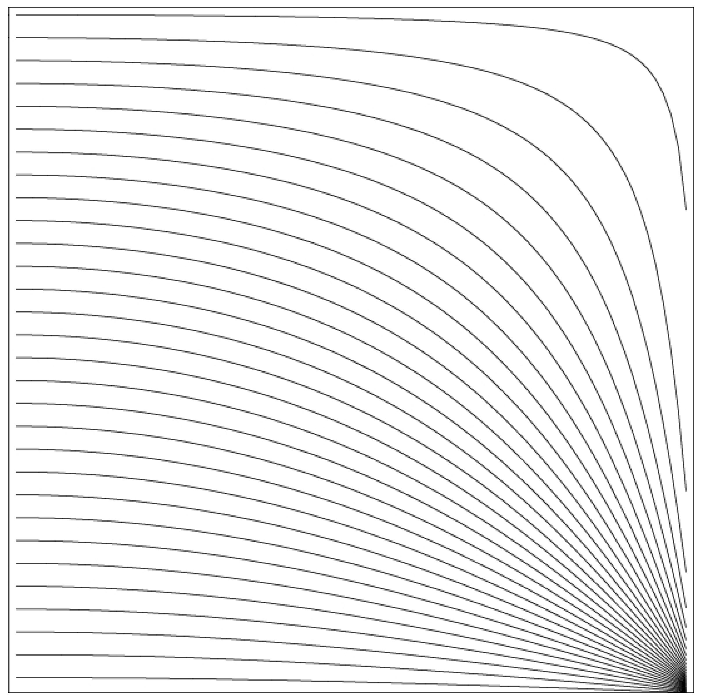
To comply with the VR systems and panorama imagery standards in use nowadays, a combination of a cylindrical roll-out in the horizontal—according to the formula (1) described and tested by Kulcke [
34]—and a torus-like roll-out in the vertical direction from a projection of an infinite orthogonal grid onto a sphere is used. This is the standard for imagery used in VR applications (see
Figure 1).
This method of unwinding the grid projected onto a sphere in two different ways (on the
x-and
y-axis in a cylindrical-like fashion and on the
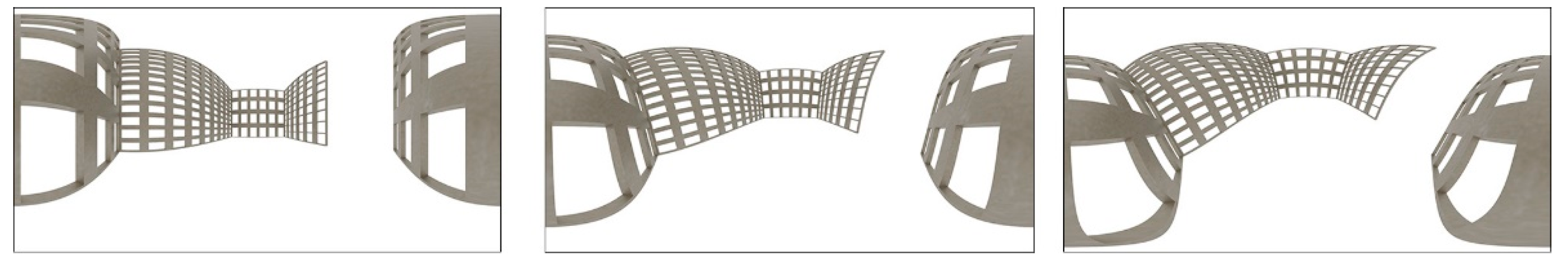
z-axis in a torus-like fashion) is yet another simplification of the reality of vision. To simplify analysis, a viewing angle axis parallel to the equatorial plane was chosen for all images undergoing box-counting. If the viewing angle axis, on the one hand, is turned around the
z-axis, then the curvature of the object edges does not change in the resulting image. If the viewing angle axis, on the other hand, is turned toward or away from the equatorial plane, then the represented edges undergo a change of curvilinear distortion, which significantly affects the results of the fractal analysis (see
Figure 2).
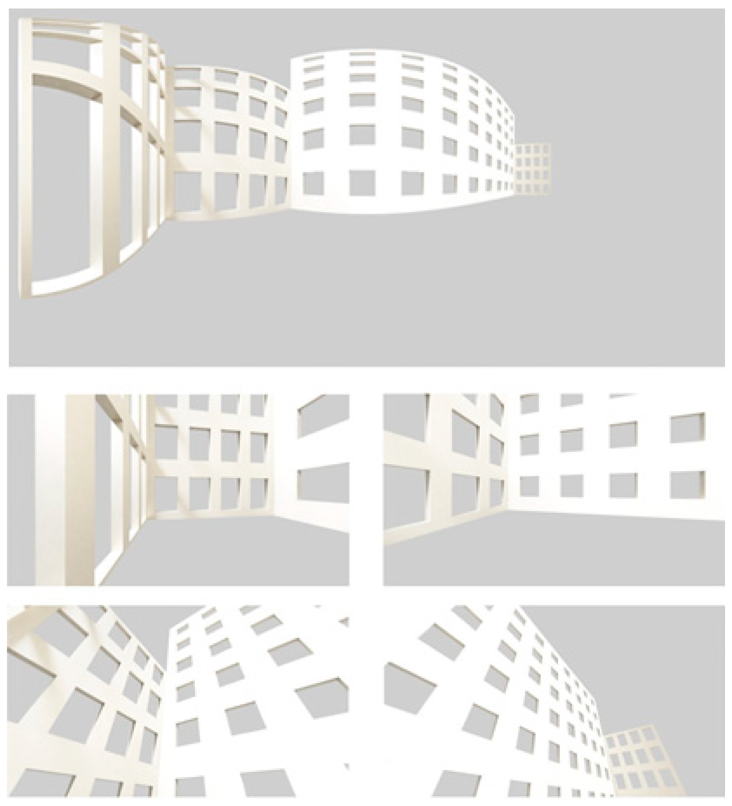
The 360-degree spherical perspective relates to the fractal by also providing potential for compression (see, e.g., [
35] (p. 458)). A 360-degree spherical perspective image contains a (theoretically) infinite amount of straight–linear perspective images (see exemplary selection in
Figure 3). These also constitute mappings with a higher degree of abstraction in relation to human perception than curvilinear perspective representations. However, this research does not evaluate which vanishing point perspective model or box-counting method does capture the actual human experience best. The 360-degree spherical perspective is thereby regarded as a specific topological fingerprint of a specific viewpoint in relation to surrounding objects, such as buildings and vegetation.
2. Materials and Methods
2.1. Box-Counting Method and Complexity
Unlike perfectly describable and smooth Euclidean figures, natural objects such as roots of trees, coastlines, and mountains are rugged and offer the same irregularity at smaller scales. Not only do fractals offer a better way to describe nature, but fractal geometry also provides methods to measure such irregularity [
3].
As mentioned in the introduction, complexity and irregularity are two characteristics of fractals. Carl Bovill was the first who related the complexity of architecture to a measurement technique called box-counting [
36]. Since then, the method has been adapted to the specifics of architectural purposes (see [
1,
5,
12,
13,
37]).
2.1.1. Standard Box-Counting and Influences on the Method
Basically, the standard box-counting method measures the distribution of black pixels’ density in a black-and-white graphic across different scales. First, a grid of square boxes is placed over the image, with the scale of the grid being indicated by the number of boxes in the bottom row. The next step is to count all of the boxes that cover parts of the image. The slope in a double logarithmic graph of scale and number of covering boxes corresponds to the box-counting dimension [
38]:
The settings or the method itself can influence the result; however, these influences can be minimized (for more information, see, e.g., [
8,
13,
39]). These influences include, for example, the first scale of the grid, i.e., the number of boxes in the bottom row. In principle, the number of starting boxes depends on the level detail in the image, with four boxes proving to be a good starting scale [
11]. The smallest scale affects the result as well. In principle, the straight part in the double logarithmic graph defines the range of scales (largest and smallest grid size), as a linear progression indicates that the two factors (scale and covering boxes) are dependent on each other. Other influences derive from the white space around the image, the reduction factor from one grid size to the next, or the position of the grid in relation to the image, as the smallest number of covering boxes per scale is looked for [
9].
2.1.2. Differential and Improved Differential Box-Counting
The standard box-counting method is well-suited for (vector-based) elevations of façades, but it has weaknesses when measuring color images or photographs in general (e.g., they have to be turned into black-and-white images using a certain threshold first). The so-called differential box-counting method [
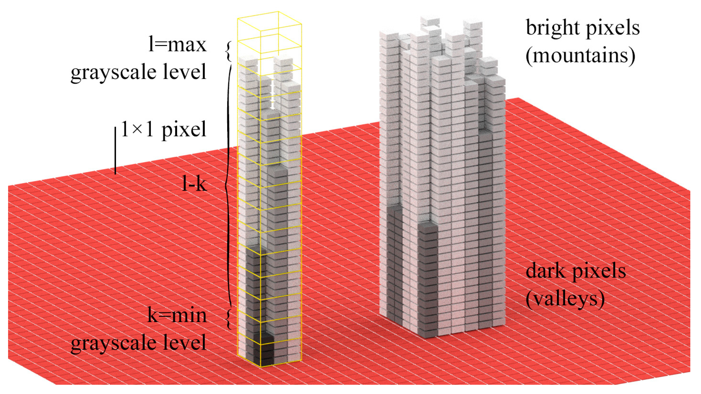
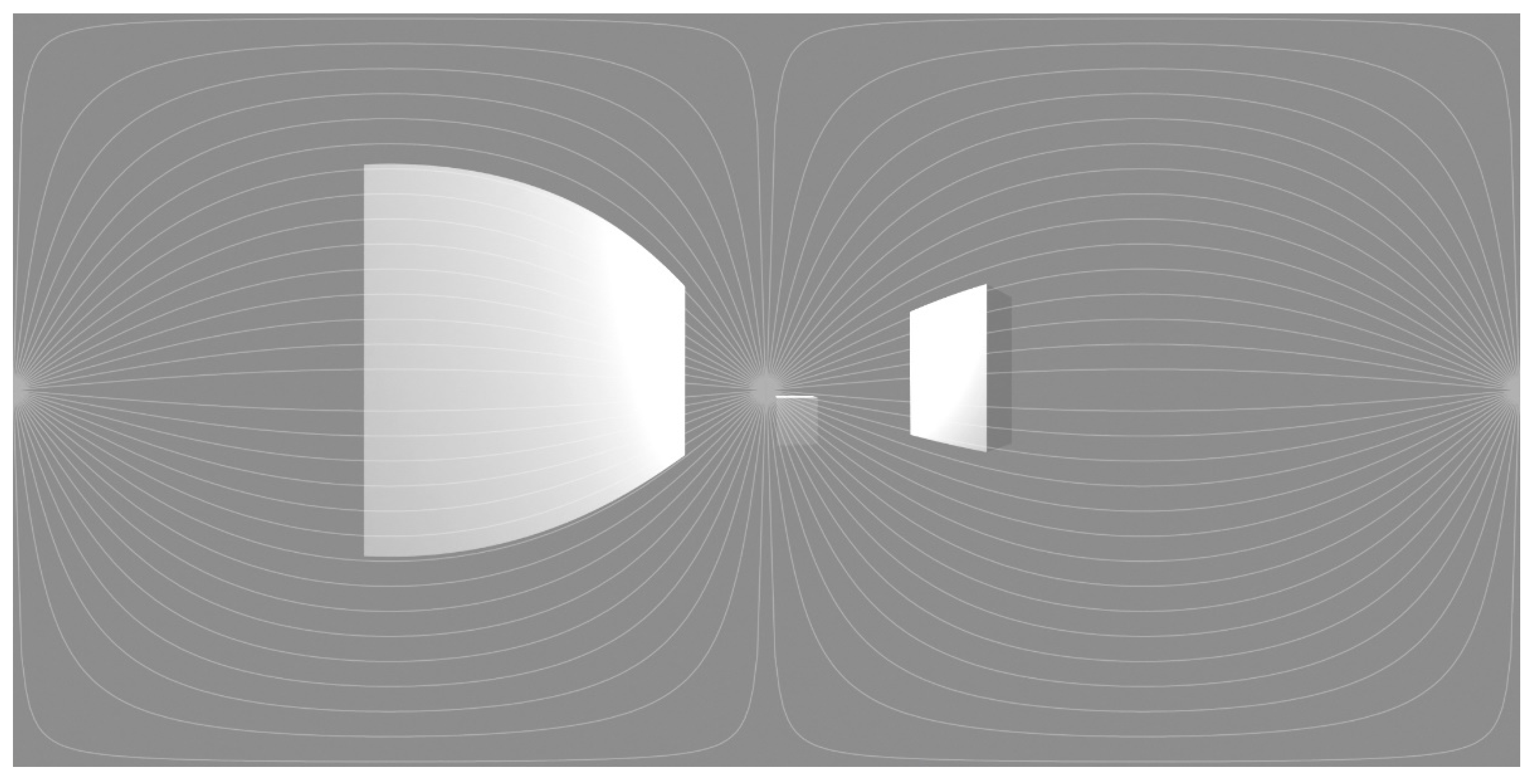
40] was developed to close the gap insofar that grayscale images can be analyzed and not just black-and-white images. With this method, the image is interpreted as a three-dimensional landscape, with the grayscale level defining the z-coordinate (see
Figure 4), where the bright pixels form the mountains and the darker pixels define the valleys. Finally, to apply the box-counting method to grayscale images, three-dimensional cubes are used for the grid instead of two-dimensional boxes; in other words, a dimension for the grayscale level is added. The size of a single cube in the grid is, therefore, (
×
×
) for a square image (
×
pixels), where (
) are pixels and (
) are grayscale levels. This results in a dependency of the value (
) on the total number of grayscale levels (
) where the following applies:
In further consequence, the number of boxes that contain a black part are not counted, but the difference between the maximum grayscale level value (
) and the minimum grayscale level value (
) is calculated for each cell (
;
) in the grid. The scale of the grid is defined by:
The difference of the minimum (
) and maximum (
) grayscale level value in one stack of cubes is given by (see
Figure 4):
Consequently, the total number of counted cubes for each grid size covering the entire image surface amounts to:
In order to be able to cover the entire range of grayscale levels, Formula (5) is modified as follows (see [
41]):
The improved differential box-counting dimension () is, finally, similar to the standard box-counting dimension given by the slope of the regression line in a double logarithmic graph with the number of counted cubes () versus grid scale () (see Formula (2)).
The results can be improved by shifting the stacks of cubes in the x and y directions [
41,
42]. In the case of stacks of cubes lying on the edge, the direction of the shift is reversed, if necessary, in order to prevent the shift from leaving the picture. Because the original position and the shifted one overlap, finally, the maximum value is searched for, which is determined as follows:
According to Long et al. [
42], four different cases occur when rectangular images (
×
pixels) are superimposed with a grid, where (
×
pixels) is the size of a single box in the grid:
× and × , indicating an even partitioning in the x- and y-directions;
× and × , indicating an uneven partitioning in the x-direction;
× and × , indicating an uneven partitioning in the y-direction;
× and × , indicating an uneven partitioning in the x- and y-directions.
In order to calculate the number (
), the base area (
) and the height (
) are added to Formula (5) as follows:
2.1.3. Differential Box-Counting for Color Images
Based on the differential box-counting method described in the previous section, the color components in a 24-bit representation of RGB color images are considered separately (Red, Green, Blue) (see [
43]). For the sake of simplicity, each color component is first converted to grayscale in order to apply the same process as before, leading to (
). The corresponding smoothness (equal to 2) is deducted from these results, leading to
Finally, all components are added to smoothness (equal to 2) again:
2.1.4. Implementation
Both the (improved) differential box-counting method for grayscale images and the (improved) differential box-counting method for color images were implemented in a web application (each for square image sections and rectangular images with shifting stacks of cubes) [
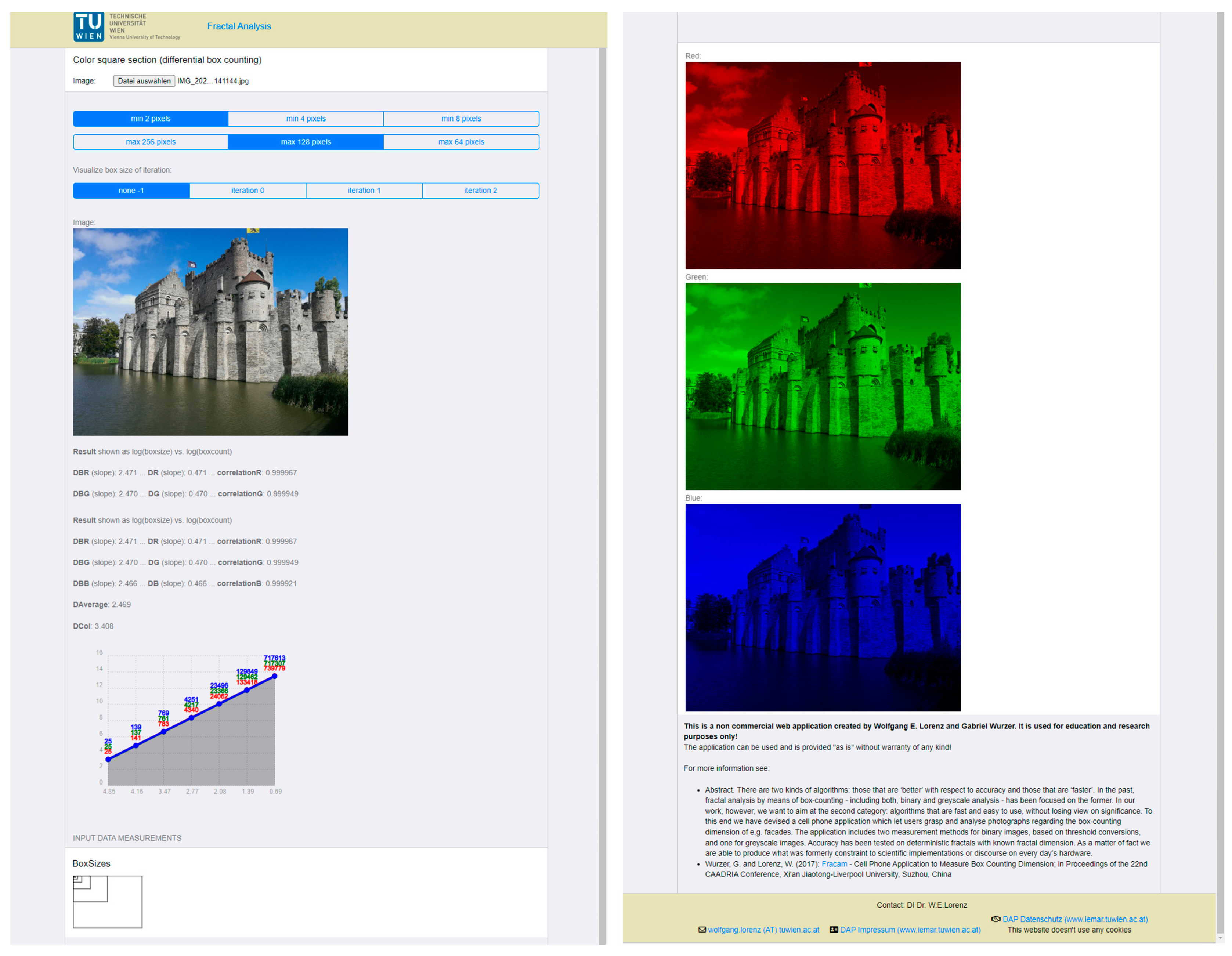
1]. FRACAM (“Fractal Camera”, first version from 2017) was initially developed to quickly analyze photographs taken with a mobile phone. This requires a balance between the qualitative output (the accuracy of the result) and the speed of the calculation (at best, in real time). For this reason, the photograph is scaled down to a maximum side length of 512 pixels. In addition, the reduction factor from one mesh size to the next is 50 percent (as a divisor of 512), which usually leads to about 6 to 8 different grid sizes per image (see
Figure 5). The lower bound of the range is user-selectable among values of 2, 4, or 8 pixels, and the upper bound is 256, 128, or 64 pixels.
FRACAM is primarily used to estimate the box count dimension (either using the standard box-counting method for black-and-white images by using a threshold or the differential box-counting applied to grayscale and color pictures either as photographs or 3D model-based renderings). We must be aware that no specific value can be assigned to a building (not least because the box-counting dimension depends on the settings, the measurement method employed, and environmental influences if photographs are used, as mentioned in the introduction); however, a building can nevertheless be described by the results of this measurement. The prerequisites are the definition of the settings and a statistical description of the deviations of the values from the regression line (see graph
Figure 5 left). This describes the continuity of a characteristic complexity over several scale ranges and the degree of complexity.
FRACAM includes the following implementation of differential box-counting (as of October 2022 after a revision):
Grayscale Images
Grayscale DBX M × M (m × m): The original photograph is reduced and cropped to a section of 512 × 512 pixels ( × ). In the case of a rectangular original image, the section can be freely selected in one direction using a slider. Because the original image is a square of 512 × 512 side lengths, the boxes of the grid are also square ( × ).
Grayscale DBX M × N (m × n): With this method, the original photograph is scaled to an image with a maximum side length of 512 pixels while maintaining the aspect ratio ( × ) and portion. Box sizes are based on the shorter side of the image. The longer side is divided by this box size and rounded down to get an integer number of boxes. The aspect ratio of a box in the grid can then also be rectangular ( × ) and not square.
Grayscale DBX
M × M (
m × m) (shifting boxes): This method is similar to the first, i.e., a square image section (
×
) is considered, and the boxes are square (
×
) as well, but this time, the stacks of cubes are moved in the x and y directions. This improves the results [
41,
42].
Grayscale DBX M × N (m × n) (shifting boxes): This method is the same as number 2 but with moved stacks of cubes.
Grayscale DBX M × N (m × m) (shifting boxes) (images will be distorted to 512 × 256): This method was developed in the year 2022 to meet the requirements of measuring spherical images. Here, the original image is adjusted to a rectangle of 512 × 256 pixels ( × ; this corresponds exactly to the aspect ratio of 1:2 of a spherical image). The box sizes, in turn, are square ( × ).
Color Images
Color DBX M × M (m × m) (shifting boxes): Analogously to method 3 of the grayscale images, a square section ( × ) is examined with a square grid ( × ).
Color DBX M × N (m × n) (shifting boxes): Analogously to method 4 of the grayscale images, the aspect ratio of the original image is preserved ( × ) and examined with a rectangular grid ( × ).
Color DBX M × N (m × m) (shifting boxes) (images will be distorted to 512 × 256): Analogously to method 5 of the greyscale images, the original image is deformed to a size of 512 × 256 pixels and examined with a square mesh.
Both groups of methods, the “Grayscale DBX” and the “Color DBX” methods, are based on the conversion of the initial image to grayscale. In the former case, the input can be a color image that is initially converted to 256 levels of gray. In the latter case, a color image is initially separated into three color channels (RGB), which are then each converted to 256 levels of gray. The default conversion is based on the average of the color components of each pixel in question:
It follows that a pure red (RGB = 255/0/0), a pure green (RGB = 0/255/0), and a pure blue (RGB = 0/0/255) image result in the same grayscale level (G = 85; brightness = 51%). A calculation of the box-counting dimension with the previously mentioned methods “Grayscale DBX” and “Color DBX” leads to a result of 2 in each case. This is because there is only one grayscale level for the entire image (i.e., there are no mountains and valleys).
Other conversion methods take into account the different perceptions of colors in relation to brightness, e.g., the weighted method, which is also called the luminosity method [
44]. This method weighs red, green, and blue according to their wavelengths. In this case, the ratio change is as follows:
In the updated 2022 version of FRACAM, it is possible to choose and apply these different calculation methods of grayscale conversion. However, one must be aware that this will produce different results because the mountains and valleys are differently pronounced.
Simplified, this calculation looks like this:
2.1.5. Surroundings and Vegetation
Applying box-counting to spherical representations rids the analysts of a crucial problem, i.e., to choose a specific frame and, thus, a certain and subjectively selected part of the architectural, topographical, and vegetational context.
2.2. Spherical Representation
To scrutinize the influence of object complexity regarding the fractal dimension in 360-degree spherical perspective images, the production of such images in CAAD software as a controlled environment was applied. The software Blender allowed for an easy export of spherical images based on a 3D model and a defined camera position and viewing angle. The default dimensions for the exported representations were changed to an image proportion of 1 to 2. To verify the underlying formula for the calculation of the image in Blender, an overlay of the spherical grid, as described by Kulcke (for more details, see [
34]), over an exported image was used for positive visual verification (
Figure 6).
2.3. Special Implications of the Method
Although straight–linear perspectives would require a plane of infinite size to entirely capture the objects and surroundings visible at a specific 360-degree viewpoint location, the spherical perspectives provide a holistic topological fingerprint. They conserve the focal angle and the direction of the center axis of the viewing angle as static representations; thus, in regard to eye or camera movement, the picture is truly arrested in time. To capture all possible foci of one location, an infinite number of finite size images would be needed (with infinitely fine resolution, as a matter of fact). Although focal directions and image expansion are both dependent on their specific resolution—the first defining the singular stepping and the second defining the number of visual units per unit of plane expanse (e.g., dpi)—the latter might take the matter of viewpoint to object distance and area-specific perspective distortion into account.
The spherical image thereby delivers a positional fingerprint representing the visual of a specific position in space, limited by location but overcoming the picture frame as a deliberate boundary. Furthermore, there is the possibility to even take the fingerprint of visual edge focus into account, as the entire system is represented by vanishing lines with changing curvature according to movement of the center of the camera angle. This change of curvature delivers a change in the fractal measure resulting from the box-counting method applied to such positional and focal fingerprints, as represented by spherical images (see
Section 1.3, Spherical Perspective Systems, and
Figure 2). The focal fingerprinting could be limited to images that represent the standard viewing angle of human beings in future research.
It is possible to merge aspects discussed from a perspective of technical feasibility with Viktor von Weizsäcker’s ideas on the circularity of trigger (Reiz), movement (Bewegung), and sensing (Wahrnehmung) [
45], which he called Gestaltkreis (Gestaltcircle). Von Weizsäcker thereby connected the detection and reception of Gestalt by human individuals with time, space, and movement. If this approach is consequently followed, a Gestalt analysis has to take these into account.
The scope of the problem of image boundaries while applying aesthetic analyses is not limited to the box-counting method. There are several other contemporary approaches that use images of architecture as a basis for calculating aesthetic measures, crowdsourcing aesthetic evaluation (e.g., [
46]), and machine learning (e.g., [
47]).
3. Results
3.1. Test Cases
As a first test of the spherical box-counting method to be implemented, several color images were examined. As explained above, a monochromatic image (such as red, green, blue, gray, white, or black) corresponds to a plane with no surface irregularities, and hence, the differential box-counting dimension is two (with a correlation value of 1.0). The situation was somewhat different when examining a checkerboard pattern, e.g., one composed of blue and black tiles. If the size of the squares of the checkerboard matched those of the grid, the differential box-counting method (without shifting stacks of cubes) led again to a result of two. Although the input corresponded to areas of different heights (the blue part being at 85 and the black part being at 0), these were located within separate lattice boxes and were thereby separated from one another.
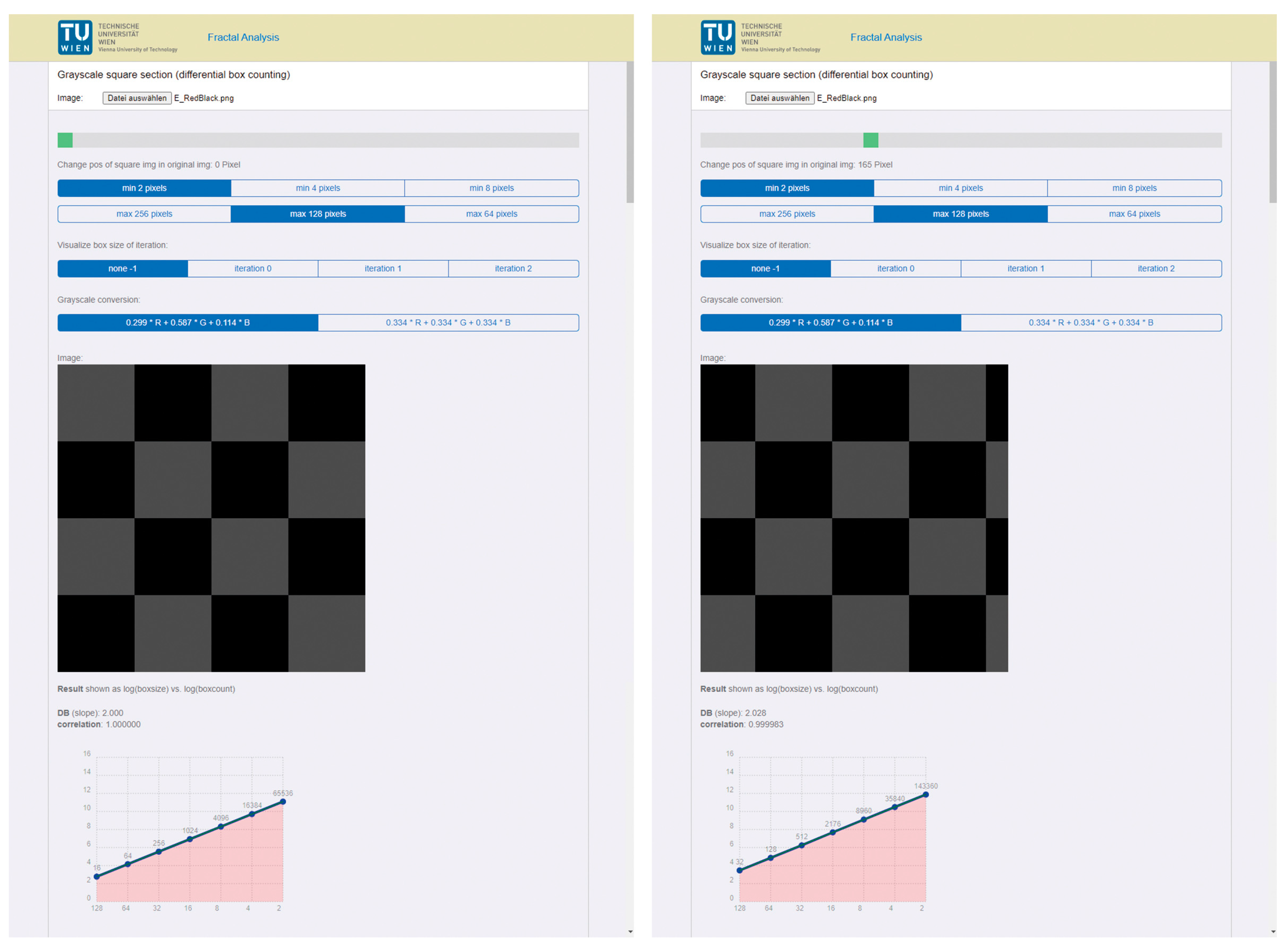
Once the checkerboard squares no longer matched those of the grid, the box-counting dimension changed. This became clear with the “Grayscale DBX
M × M (
m × m)” method—in which only a square section is considered—when the section was shifted accordingly (see
Figure 7).
With the improved method for grayscale images, in which the stacks of cubes are shifted, the result was slightly higher than 2, namely 2.093 (with a correlation value of 0.999769 for the standard grayscale conversion). With the weighted grayscale conversion, the value changed to 2.142 (with a correlation value of 0.999597). The application of the color measurement methods that separate the color components led to similar results. Because the chessboard consisted of blue and black tiles in our example, the box-counting dimension for the red and green components was 2 each, whereas the results for the blue component were, again, 2.093 and 2.142, respectively.
Looking at the checkerboard from before with the black tiles replaced by white ones, the results changed as the black valleys were replaced by white mountains. With the color method (that is, dividing the image into the three color components that accord to the RGB color model), the results changed again because white light contains all three colors in RGB. For the blue component, the box-counting dimension was two because both the blue and white tiles contained the maximum blue value (that is, equal to a plane). The other two color components again resulted in 2.093 (with the standard grayscale conversion), the same value as before, because the blue tile now constituted a black valley.
3.1.1. Simple Parametrical CAD Models
As a first approximation and test case, a rectangular courtyard situation was examined. The setting was parameterized using a script in a CAAD program so instances with specific variations (in sizes, number of façade openings, etc.) could be analyzed in comparison. Basically, the yard placement was characterized by four enclosures (representing building fronts) with the side being partially opened, whereas the distances in between buildings (i.e., the size of the courtyard), the heights of the building fronts, and the proportions of the window openings could vary. The starting point of the building fronts (x, y, z), their depths, edge distances, heights, widths, and rotations could be set. Furthermore, the façade openings could be defined by the distances in horizontal and vertical directions according to façade orientation and by the number of rows and columns. All of these definitions were set via a CSV file (comma-separated values).
A total of six different square situations were examined with variations in courtyard sizes as well as complexities of the façades (due to different window proportions). The configurations themselves were simple, taking only the proportions of the façade and the windows into account (leaving ornaments and finer details aside). Each of the 360-degree spherical images were adjusted in terms of color (façades in red, green, or blue), gray levels (façades in light gray or dark gray), and in terms of background (white or black) to address their degree of impact. In this way, 120 measurements were carried out, 60 each for the standard grayscale conversion (one-third share for the color channels, see Formula (12)) and for the conversion adapted to the perception of brightness (see Formula (13)).
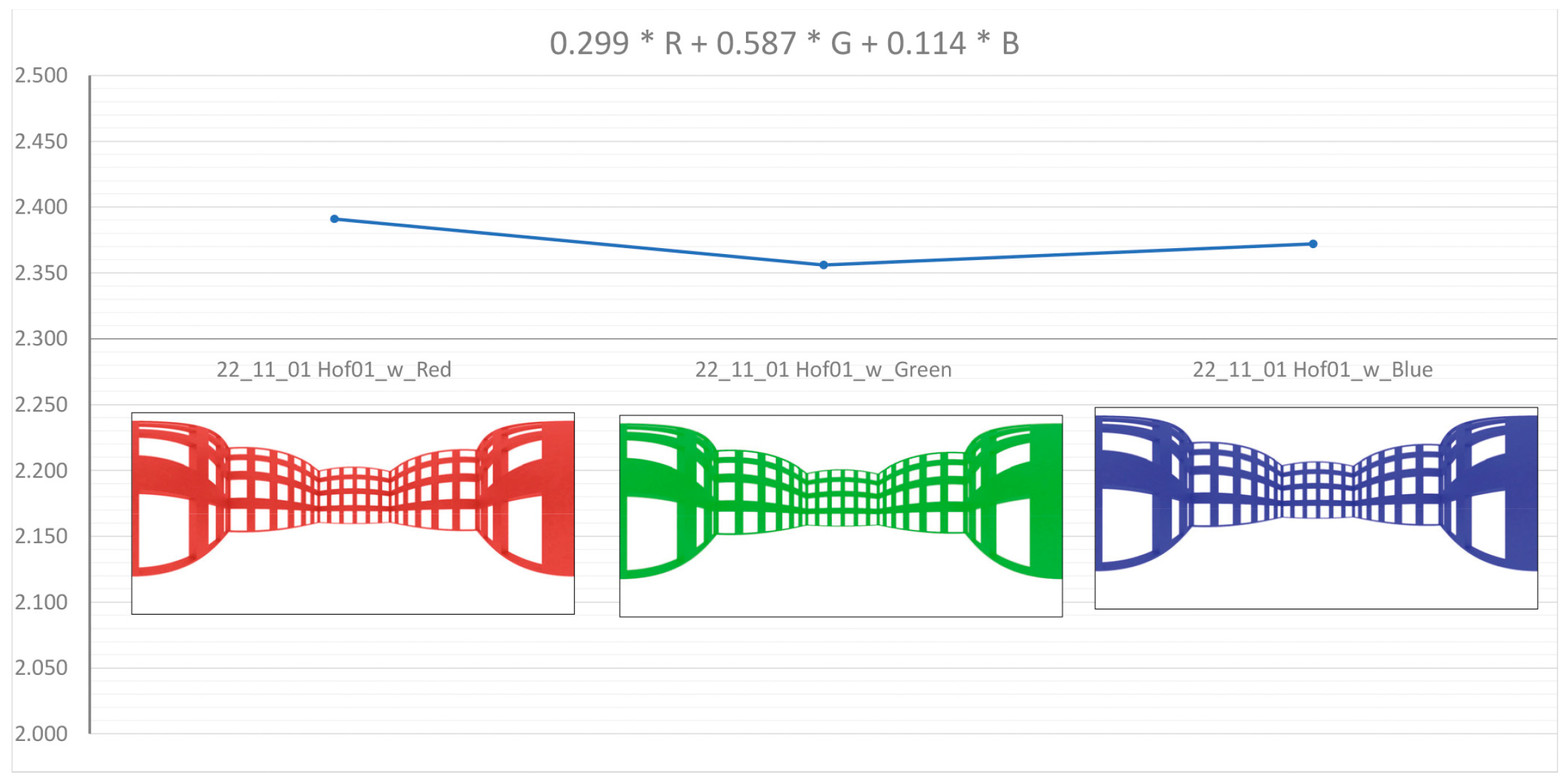
First, the grayscale calculation was performed with the previously described algorithm “Grayscale DBX
M × N (
m × m) (shifting boxes)”. It turned out that for the versions of façades colored with different gray values, there are only minor differences between the two different grayscale conversions. In turn, and as expected, there were differences in the colored façades because the weighting of the brightness of the three color channels influenced the result but not the tendencies. The red-colored façades achieved the highest values, whereas the green ones achieved the lowest ones (see
Figure 8).
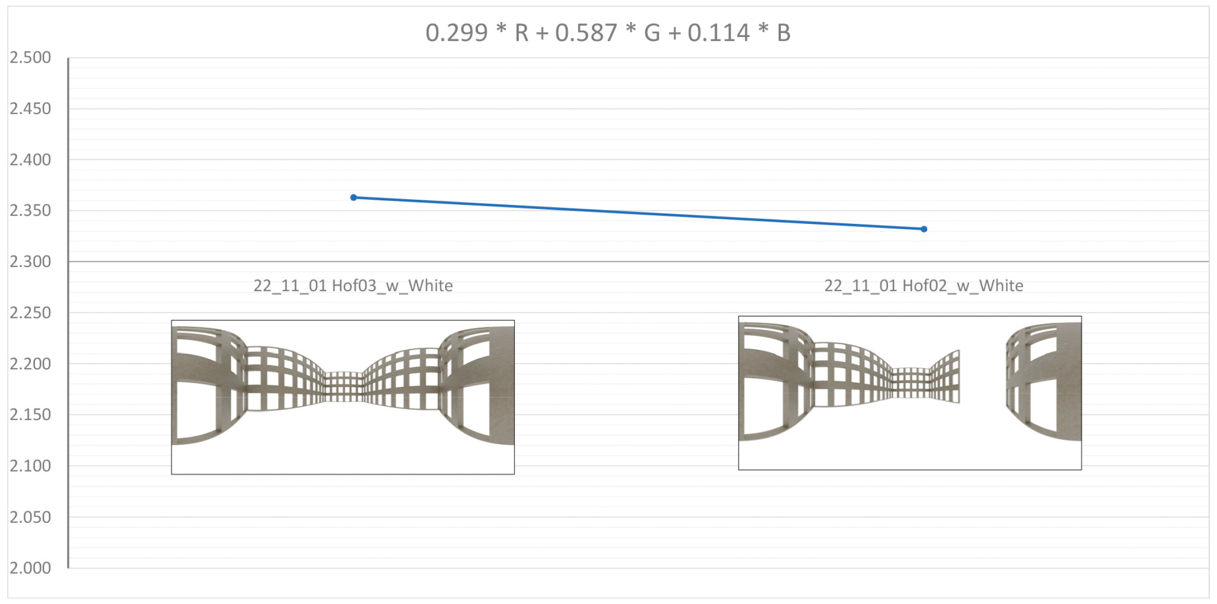
Closed and partially open courtyards showed differences even if the opening was small, with the former resulting in higher box-counting dimensions than the latter (see
Figure 9).
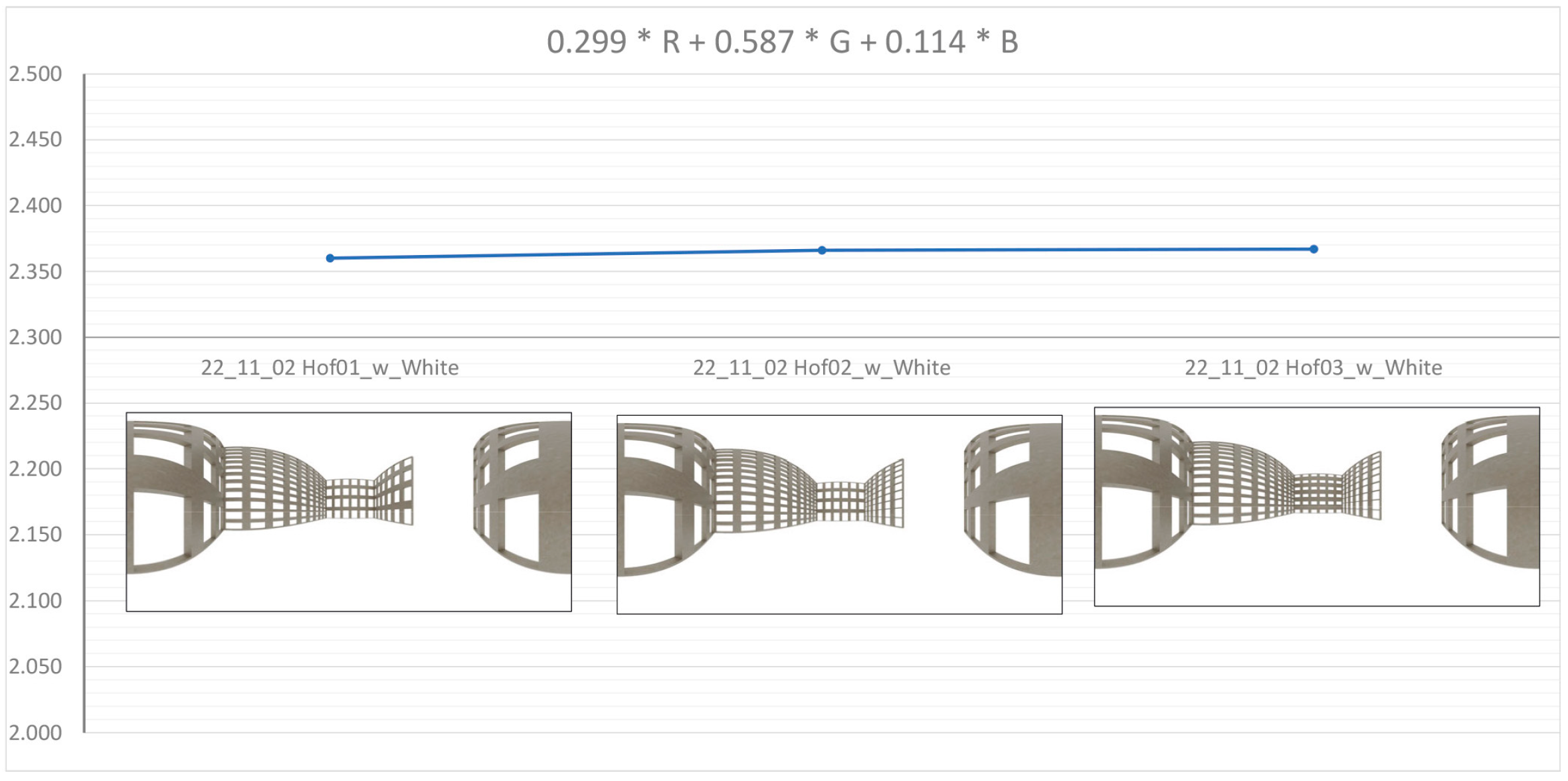
Changing the window proportions of just a few façades within the same courtyard (with otherwise unchanged façades) led only to small differences in the results. As can be seen in
Figure 10, the box-counting dimension increased only marginally as more rows of windows were introduced, with the number of windows increasing while their height decreased.
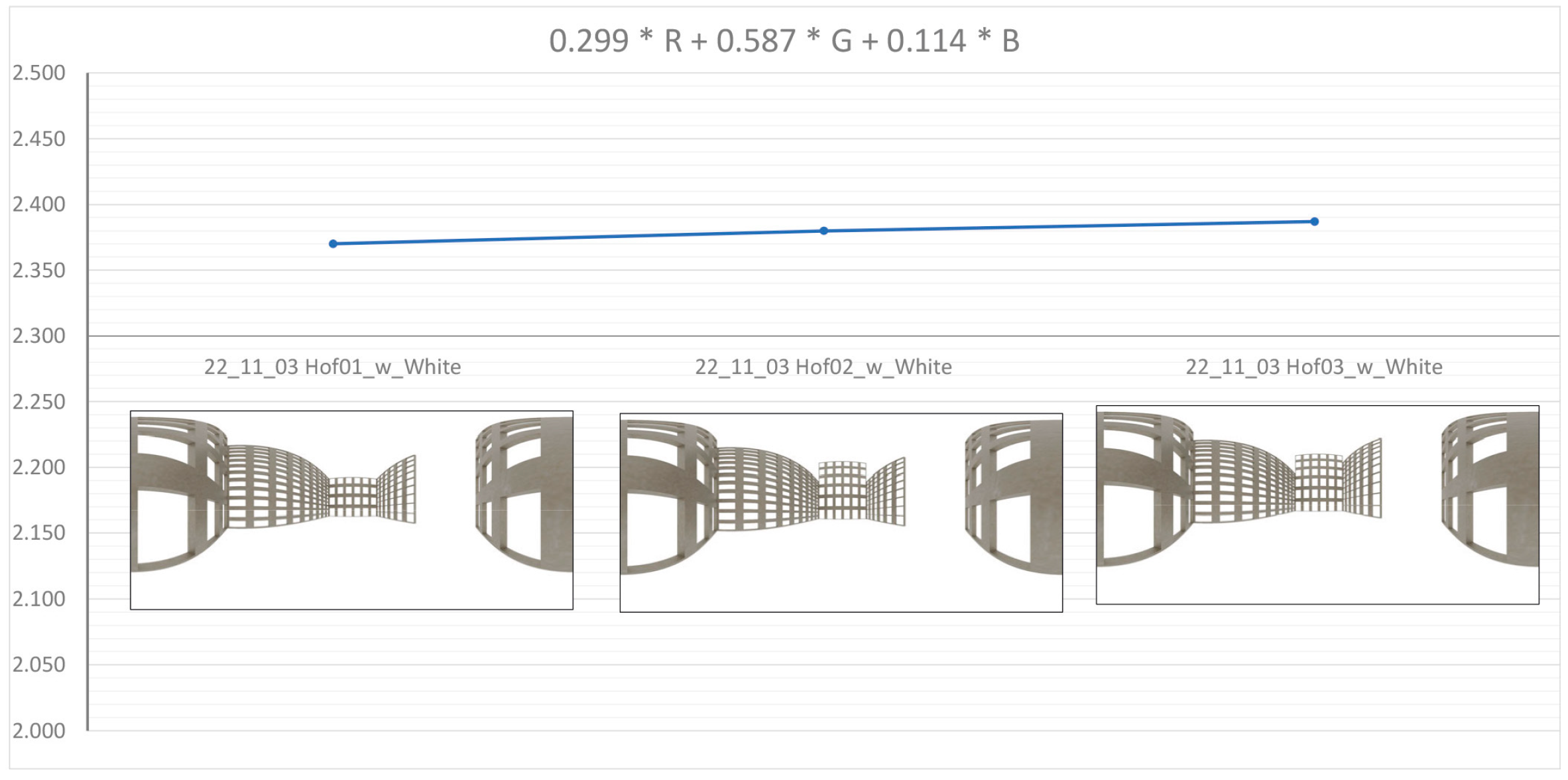
After the first round of analysis, another three comparative measurements were carried out on different configurations of instances of the surrounding façades of the courtyard. This time, the heights of some adjacent façades were changed, which led to corresponding changes in the results. In a first step, the height of the façade opposite the camera was increased in comparison with the reference example, and an additional row of windows was added. After that, an adjacent façade was also raised. Using the grayscale method with adapted grayscale conversion (see Formula (13)), the box-counting dimensions increased accordingly from 2.37 for the original image to 2.38 after the first change and finally to 2.387 (see
Figure 11).
3.1.2. Spherical Photographs
After the parametric test cases were completed, a total of 13 spherical photographs were analyzed. These examples originated from a field trip to Chicago and the surrounding areas in 2019 [
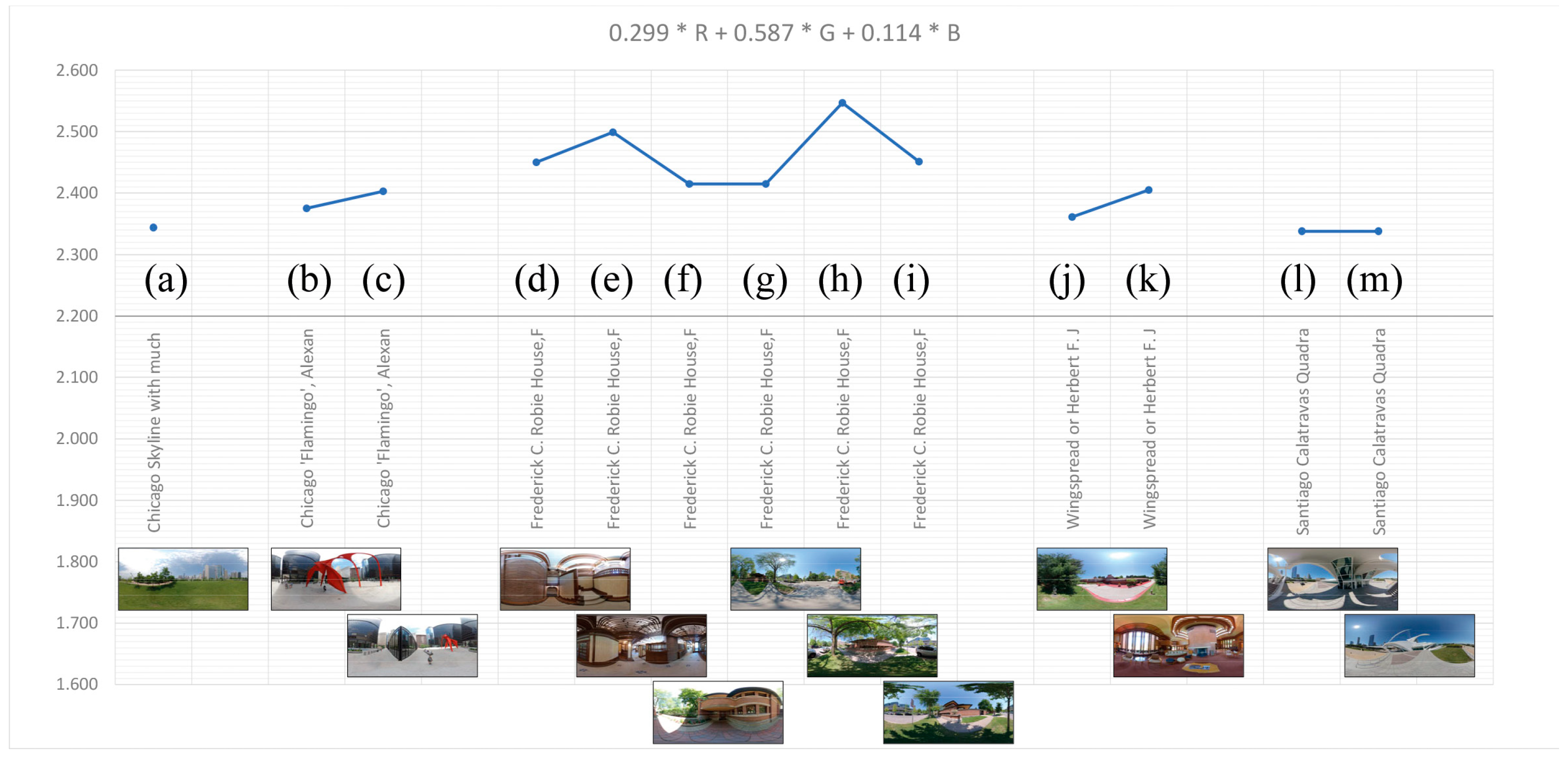
48]. The selected motifs ranged from the Chicago skyline with a considerable portion of surrounding greenery to typical examples of the prairie style of Frank Lloyd Wright with its earthy tones showing both outside and inside, leading up to an example by Santiago Calatrava with large areas of white and a large area of the image taken up by (blue) sky. With these images, the application of the grayscale calculation of the adjusted conversion showed a clear tendency. Those examples that contained greater areas of similar color, either in the form of a high percentage of sky or greenery but also in the form of uniform coloring on these buildings, as was the case with the Calatrava example, had the lowest box-counting dimensions, as presented in
Figure 12:
Figure 12a: “Chicago Skyline” with a large portion of greenery,
;
Figure 12b: Federal Center Plaza in Chicago with the “Flamingo” by Alexander Calder from 1974, with a large portion of a uniform-colored plaza and a red colored sculpture in the foreground,
;
Figure 12j: the Wingspread or Herbert F. Johnson House by Frank Lloyd Wright from 1937 in Wind Point, Wisconsin, with a considerable amount of greenery,
;
Figure 12l: Quadracci Pavilion by Santiago Calatrava from 2001 in the Milwaukee Art Museum, Wisconsin, with a large portion of uniform floor design and similarly colored building areas,
;
Figure 12m: the same white-colored building with a large portion of blue sky and uniform floor design,
.
The exterior view of Frank Lloyd Wright’s Robie House achieved the highest result (see
Figure 12h). The front view of the building with exposed red bricks and horizontal stripes of gray stone formed the center of the image, and in the foreground, a narrow strip of green alternated with the light gray of the pavement. The surrounding trees added further contrast through the color of the trunk and the shade of the leaves. All of this led to a box-counting dimension of
. The interior views (d) and (e) also achieved a high degree of variation (
and
).
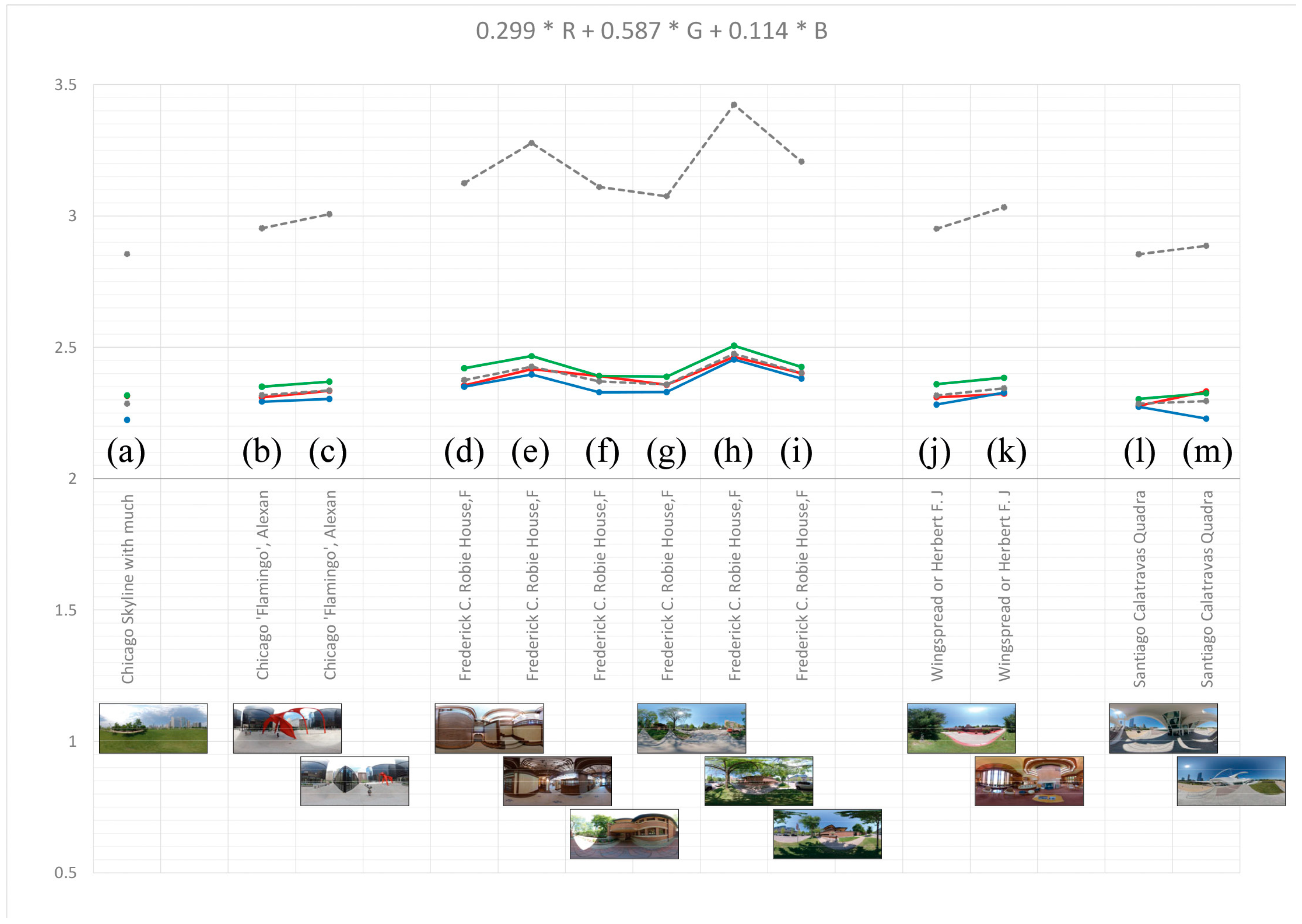
Applying the color measurement method “Color DBX
M × N (
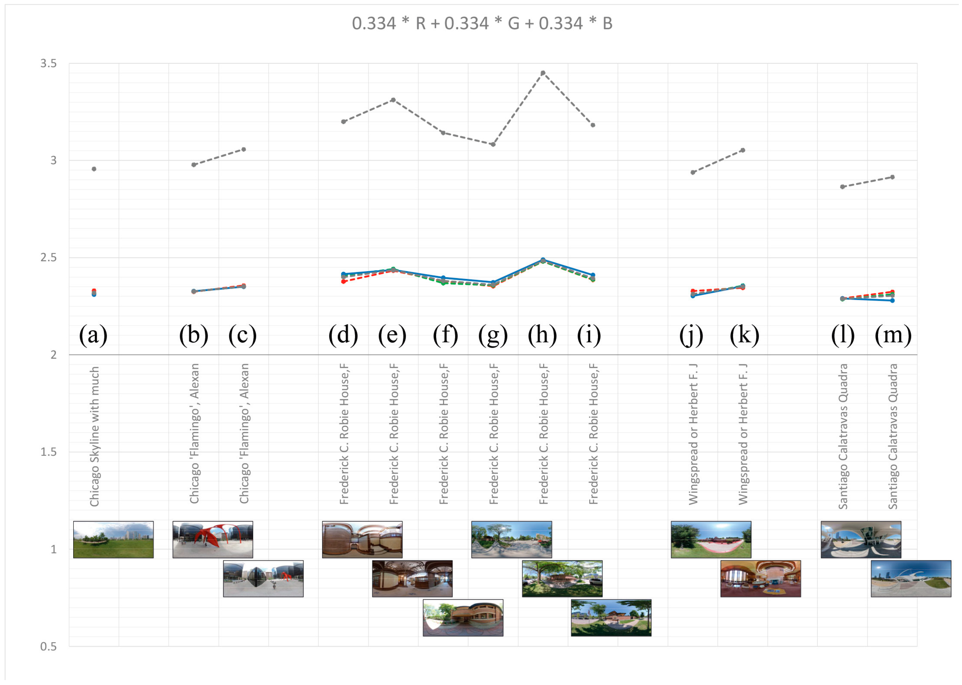
m × m) (shifting boxes)” to the same selection of architectural examples led to similar tendencies as the previous analysis with the grayscale measurement method. An alike variation as before occurred for the color channels (Red, Green, Blue), whereas
resulted in an even clearer difference between each architectural example, with the exterior front view of Robie House reaching the absolute highest score,
(see
Figure 13). It is worth noting that using the adapted grayscale conversion led to the lowest results for the blue color channel, especially when the portion of blue sky was large (see
Figure 13m). In contrast, the green color channel showed the highest values, and not only for those examples that had a high portion of greenery. With the standard grayscale conversion of the color components, the values for the individual color channels contracted, i.e., the differences became smaller (see
Figure 14). Though, the example by Calatrava (see
Figure 13m and
Figure 14m) with a larger portion of blue sky again showed a lower value for the blue channel, albeit not as clearly. On the other hand, the blue channel of the Robie House usually had higher values than the other color channels.
Compared to the other examples, the interior spherical images of the Robie House achieved relatively high values (see
Figure 13d,e and
Figure 14d,e). This supports the hypothesis that the Robie House exhibits a higher degree of complexity across many scales due to its design. For example,
Figure 13e and
Figure 14e shows a richly decorated ceiling, plastered wall surfaces that alternate with exposed bricks and wooden elements, and a uniform carpet on the floor that has individual patterns and an edge stripe.
In any case, what became clear is that both the design of the building and the character of the surroundings have an impact on the result. Thus,
Figure 13h and
Figure 14h had a high
, whereas
Figure 13a,m and
Figure 14a,m had the lowest values. The former shows both the high complexity of the building itself with exposed bricks, stone-made horizontal wall endings, a certain angle in various elements from the “bow” to the glass window designs, and widely projecting flat roofs [
49], as well as of the environment with foliage, sidewalks, and various surrounding buildings. Conversely,
Figure 13a,m and
Figure 14a,m contained large areas of greenery and sky, respectively, and buildings with less color variation.
4. Discussion
In the past, the aesthetic evaluation of architecture was essentially focused on proportion theories and/or color theories that were developed over the centuries in the fields of architecture and fine arts. It is common knowledge that, e.g., certain proportions as the golden section were (and are still) considered vital for a successful building design or a harmonious piece of art by professionals and recipients alike. In modern design theory, a more holistic view integrates these and other approaches dealing with the question of aesthetic quality, especially aesthetic harmony, focusing on the balance between order and irregularity or, in other terms, between simplicity and complexity (see e.g., [
50,
51]).
In recent years, it can be shown that useful analysis methods were spawned by the relatively young branch of fractal theory to measure characteristic degrees of complexity within objects under scrutiny. Box-counting, as one of them, was originally applied to black-and-white images and primarily focuses on examining complexity as an expression of density distribution from large to small scales. In the present study, grayscale as well as color images of architecture were interpreted, taking brightness as 3D landscapes with similarity to mountains and valleys into account and thereby extending the box-counting method, which was previously limited to two-dimensional representations of, e.g., façades as line graphics, to 2.5 dimensions. Together with the examination of 360-degree spherical panorama images, for the first time, the building in its entire context was examined. This observer location-based approach minimizes the influence of the image selection in relation to the grid, whereas the standardized 1:2 aspect ratio of the panorama images accommodates the square-shaped boxes of the grid.
The method presented here to scrutinize architecture in its environment through the application of box-counting to 360-degree spherical perspective imagery produced the same tendencies considering resulting box-counting dimensions that were expected by the authors. The instances of courtyard-like situations constructed with the help of CAAD models organized in a parametric fashion for individual configuration allowed for testing changes in courtyard expanse, façade height, and façade-complexity (through altering the size and distribution of openings).
In the future, the use of specific box-counting grids with three or more sizes of boxes within one grid are to be tested as a potential way to further improve the method.
5. Conclusions and Outlook
A method to analyze architecture in its surroundings was tested, but it still remains to develop a method to identify significant observer positions according to the characteristics of buildings in their environment. This aspect goes beyond fractal analysis, as it can be considered a vital part of the groundwork for applying all methods of Gestalt analyses on objects in space more successfully.
With FRACAM—an easy-to-use website application to measure the box-counting dimensions of grayscale and color images—it is shown that the measurement of 360-degree spherical panorama images is less susceptible to influences attributable to the measurement method itself, e.g., when using black-and-white elevation drawings, which were previously used to analyze buildings. This is mainly due to the fact that the entire 360-degree scenery is taken into account, thereby avoiding influence due to a specific image frame selection. Owing to this improvement of the method, it is no longer necessary to add white (empty) space around the selection of the image and shift the grid accordingly.
It is also shown that even minor changes in the complexity of the analyzed environment, such as raising one or more buildings or adding rows of windows, can be read from the results. Furthermore, the effect of converting RGB color images to grayscale images inherent in the different implemented methods was studied using two methods (the default one-third conversion method and the luminosity method, each with different weighting of the color components), which yielded slightly different results but showed, however, similar tendencies.
So far, only a few initial examples of architecture have been examined, but further measurements need to be carried out to allow putting the results into a broader context. In the future, a series of 360-degree spherical panorama images that use the same location at different times of the day and season will also be examined. Doing so will make it possible to classify different scenarios or buildings in relation to one another and to iconic architecture, with observer locations being provided in an accompanying database.
Author Contributions
Conceptualization, W.E.L. and M.K.; methodology, W.E.L. and M.K.; software “FRACAM”, W.E.L.; validation, W.E.L. and M.K.; formal analysis, W.E.L. and M.K.; investigation, W.E.L. and M.K.; resources, W.E.L. and M.K.; data curation, W.E.L. and M.K.; writing—original draft preparation, W.E.L. and M.K.; writing—review and editing, W.E.L. and M.K.; visualization, W.E.L. and M.K. All authors have read and agreed to the published version of the manuscript.
Funding
This research received no external funding.
Data Availability Statement
Acknowledgments
We thank Arnold Faller for the 360-degree photographs provided and Gabriel Wurzer for contributions to FRACAM.
Conflicts of Interest
The authors declare no conflict of interest.
References
- Lorenz, W.E.; Wurzer, G. FRACAM: A 2.5D Fractal Analysis Method for Facades Test Environment for a Cell Phone Application to Measure Box-counting Dimension. In Proceedings of the eCAADe 2020, Berlin, Germany, 16–18 September 2020; pp. 495–504. [Google Scholar] [CrossRef]
- Mandelbrot, B.B. Scalebound or scaling shapes: A useful distinction in the visual arts and in the natural sciences. Leonardo 1981, 14, 45–47. [Google Scholar] [CrossRef]
- Mandelbrot, B.B. The Fractal Geometry of Nature; W.H. Freeman: San Francisco, CA, USA, 1982. [Google Scholar]
- Jencks, C. The Architecture of the Jumping Universe; Wiley & Sons: Chichester, UK, 1995. [Google Scholar]
- Lorenz, W.E. Fractals and Fractal Architecture. Master’s Thesis, TU Wien (Vienna University of Technology), Vienna, Austria, 2003. [Google Scholar]
- Franck, G.; Franck, D. Architektonische Qualität; Hanser: München, Germany, 2008. [Google Scholar]
- Salingaros, N.A. A Theory of Architecture; Umbau Verlag: Solingen, Germany, 2006. [Google Scholar]
- Lorenz, W.E.; Andres, J.; Franck, G. Fractal Aesthetics in Architecture. Appl. Math. Inf. Sci. 2017, 11, 971–981. [Google Scholar] [CrossRef]
- Peitgen, H.-O.; Jürgens, H.; Saupe, D. Chaos and Fractals—New Frontiers of Science; Springer: New York, NY, USA, 1992. [Google Scholar]
- Corbit, J.D.; Garbary, D.J. Fractal dimension as a quantitative measure of complexity in plant development. Proc. R. Soc. Lond. B 1995, 262, 1–6. [Google Scholar] [CrossRef]
- Foroutan-pour, K.; Dutilleul, P.; Smith, D.L. Advances in the implementation of the box-counting method of fractal dimension estimation. Appl. Math. Comput. 1999, 105, 195–210. [Google Scholar] [CrossRef]
- Ostwald, M.J.; Vaughan, J. The Fractal Dimension of Architecture; Birkhäuser: Basel, Switzerland, 2016. [Google Scholar]
- Lorenz, W.E.; Kulcke, M. Multilayered Complexity Analysis in Architectural Design: Two Measurement Methods Evaluating Self-Similarity and Complexity. Fractal Fract. 2021, 5, 244. [Google Scholar] [CrossRef]
- Vaughan, J.; Ostwald, M.J. The comparative numerical analysis of nature and architecture: A new framework. Int. J. Des. Nat. Ecodyn. 2017, 12, 156–166. [Google Scholar] [CrossRef]
- Alberti, L.B. The Ten Books of Architecture: The 1755 Leoni Edition; Dover: New York, NY, USA, 1986. [Google Scholar]
- Von Goethe, J.W. Zur Farbenlehre; der J. G. Cotta’schen Buchhandlung: Tübingen, Germany, 1810. [Google Scholar]
- Itten, J. Kunst der Farbe: Subjektives Erleben und Objektives Erkennen als Wege zur Kunst; Otto Maier Verlag: Ravensburg, Germany, 1961. [Google Scholar]
- Wittkower, R. Architectural Principles in the Age of Humanism; Tiranti: London, UK, 1962. [Google Scholar]
- Corbusier, L. Towards a New Architecture; J. Rodker: London, UK, 1931. [Google Scholar]
- Mandelbrot, B.B. Les Objets Fractals: Forme Hasard Et Dimension; Flammarion: Paris, France, 1975. [Google Scholar]
- Batty, M.; Longley, P. Fractal Cities; Academic Press Inc.: London, UK, 1994. [Google Scholar]
- Bunde, A. Fractals in Science: With a MS-DOS Program Diskette; Springer: Berlin, Germany, 1994. [Google Scholar]
- Zebari, D.A.; Ibrahim, D.A.; Zeebaree, D.Q.; Mohammed, M.A.; Haron, H.; Zebari, N.A.; Damaševičius, R.; Maskeliūnas, R. Breast Cancer Detection Using Mammogram Images with Improved Multi-Fractal Dimension Approach and Feature Fusion. Appl. Sci. 2021, 11, 12122. [Google Scholar] [CrossRef]
- Huang, P.; Li, D.; Zhao, H. An Improved Robust Fractal Image Compression Based on M-Estimator. Appl. Sci. 2022, 12, 7533. [Google Scholar] [CrossRef]
- Mandelbrot, B.B. Fractals: Form Chance and Dimension; W.H. Freeman: San Francisco, CA, USA, 1977. [Google Scholar]
- Mandelbrot, B.B. Fractals and an Art for the Sake of Science. Leonardo 1989, 2, 21–24. [Google Scholar] [CrossRef]
- Ryu, K.; Jung, M. Agent-based fractal architecture and modelling for developing distributed manufacturing systems. Int. J. Prod. Res. 2003, 41, 4233–4255. [Google Scholar] [CrossRef]
- Baldini, G.; Amerini, I. Online Distributed Denial of Service (DDoS) intrusion detection based on adaptive sliding window and morphological fractal dimension. Comput. Netw. 2022, 210, 108923. [Google Scholar] [CrossRef]
- Mandelbrot, B.B. How long is the coast of Britain? Statistical self-similarity and fractional dimension. Science 1967, 156, 636–638. [Google Scholar] [CrossRef] [PubMed]
- Jiang, B.; Yin, J. Ht-Index for Quantifying the Fractal or Scaling Structure of Geographic Features. Ann. Assoc. Am. Geogr. 2014, 104, 530–540. [Google Scholar] [CrossRef]
- Bateson, G. Mind and Nature: A Necessary Unity; Bantam Books: New York, NY, USA, 1988. [Google Scholar]
- Misra, R.P.; Ramesh, A. Fundamentals of Cartography, 2nd ed.; Concept Publishing Company: New Delhi, India, 1989. [Google Scholar]
- Arnheim, R. Kunst und Sehen: Eine Psychologie des Schöpferischen Auges; De Gruyter: Berlin, Germany; Boston, MA, USA, 2000. [Google Scholar] [CrossRef]
- Kulcke, M. Spherical Perspective in Design Education. FME Trans. J. 2019, 47, 343–348. [Google Scholar] [CrossRef]
- Nelson, M.; Gaily, J.L. The Data Compression Book, 2nd ed.; M&T Books: New York, NY, USA, 1996. [Google Scholar]
- Bovill, C. Fractal Geometry in Architecture and Design; Birkhäuser: Boston, MA, USA, 1996. [Google Scholar]
- Vaughan, J.; Ostwald, M.J. Refining the Computational Method for the Evaluation of Visual Complexity in Architectural Images—Significant Lines in the Early Architecture of Le Corbusier. In Proceedings of the eCAADe 2009, Computation: The New Realm of Architectural Design, Istanbul, Turkey, 16–19 September 2009; pp. 686–696. [Google Scholar] [CrossRef]
- Falconer, K.J. Fractal Geometry: Mathematical Foundations and Applications; Wiley: New York, NY, USA, 2003. [Google Scholar]
- Ostwald, M.J. The Fractal Analysis of Architecture: Calibrating the Box-Counting Method Using Scaling Coefficient and Grid Disposition Variables. Environ. Plan. B Plan. Des. 2013, 40, 644–663. [Google Scholar] [CrossRef]
- Sarker, N.; Chaudhuri, B.B. An efficient differential box-counting approach to compute fractal dimension of image. IEEE Trans. Syst. Man Cybern. 1994, 24, 115–120. [Google Scholar] [CrossRef]
- Liu, Y.; Chen, L.; Wang, H.; Jiang, L.; Zhang, Y.; Zhao, J.; Wang, D.; Zhao, Y.; Song, Y. An improved differential box-counting method to estimate fractal dimensions of gray-level images. J. Vis. Commun. Image Represent. 2014, 25, 1102–1111. [Google Scholar] [CrossRef]
- Long, M.; Peng, F. A Box-Counting Method with Adaptable Box Height for Measuring the Fractal Feature of Images. Radioengineering 2013, 22, 208–213. [Google Scholar]
- Nayak, S.R.; Mishra, J. On Calculation of Fractal Dimension of Color Images. Int. J. Image Graph. Signal Process. (IJIGSP) 2017, 9, 33–40. [Google Scholar] [CrossRef]
- Kanan, C.; Cottrell, G.W. Color-to-Grayscale: Does the Method Matter in Image Recognition? PLoS ONE 2012, 7, e29740. [Google Scholar] [CrossRef]
- Weizsäcker, V.V. Der Gestaltkreis. Theorie der Einheit von Wahrnehmen und Bewegen; Suhrkamp Verlag: Frankfurt am Main, Germany, 1973. [Google Scholar]
- Sardenberg, V.; Becker, M. Computational Quantitative Aesthetics Evaluation: Evaluating architectural images using computer vision, machine learning and social media. In Proceedings of the eCAADe 2022, Ghent, Belgium, 13–16 September 2022; Volume 2, pp. 567–574. [Google Scholar]
- Eroğlu, R.; Gül, L.F. Architectural Form Explorations through Generative Adversarial Networks—Predicting the potentials of StyleGAN. In Proceedings of the eCAADe 2022, Ghent, Belgium, 13–16 September 2022; Volume 2, pp. 575–582. [Google Scholar]
- Lorenz, W.E.; Faller, A. (Eds.) Exkursion Chicago 2019; TU Wien E259-01 Architekturwissenschaften—Digitale Architektur und Raumplanung: Vienna, Austria, 2019. [Google Scholar]
- Hoffmann, D. Robie House; Dover Publications: New York, NY, USA, 1984. [Google Scholar]
- Birkhoff, G.D. Aesthetic Measure; Harvard University Press: Cambridge, MA, USA, 1933. [Google Scholar]
- Bense, M. Zeichen und Design—Semiotische Ästhetik; Agis-Verlag: Baden Baden, Germany, 1971. [Google Scholar]
Figure 1.
Partial spherical grid produced on the basis of Formula (1) [
34].
Figure 1.
Partial spherical grid produced on the basis of Formula (1) [
34].
Figure 2.
Changing the viewing angle axis leads to curvilinear distortion.
Figure 2.
Changing the viewing angle axis leads to curvilinear distortion.
Figure 3.
Four straight–linear perspectives calculated in GoPro® VR player 3.0.5 software on the basis of a 360-degree spherical perspective image created with Blender® 3.3.0 software.
Figure 3.
Four straight–linear perspectives calculated in GoPro® VR player 3.0.5 software on the basis of a 360-degree spherical perspective image created with Blender® 3.3.0 software.
Figure 4.
Differential box-counting method for grayscale images. The yellow highlighted stack of cubes shows the difference between the brightest and darkest pixel for one specific cell (i;j) of a certain grid size.
Figure 4.
Differential box-counting method for grayscale images. The yellow highlighted stack of cubes shows the difference between the brightest and darkest pixel for one specific cell (i;j) of a certain grid size.
Figure 5.
Differential box-counting of the web application “FRACAM”, showing the castle of Ghent, Belgium. (Left top, left middle): results, with = 0.471, = 0.470, and = 0.466; with = 0.471, = 0.999949, and = 0.999921; = 2.469; = 3.408; (left bottom): used box sizes; (right side): RGB separation.
Figure 5.
Differential box-counting of the web application “FRACAM”, showing the castle of Ghent, Belgium. (Left top, left middle): results, with = 0.471, = 0.470, and = 0.466; with = 0.471, = 0.999949, and = 0.999921; = 2.469; = 3.408; (left bottom): used box sizes; (right side): RGB separation.
Figure 6.
Spherical perspective rendering produced in Blender with an overlay of curves representing the first and third dimensions according to the formula in [
34] (cylindrical roll-out) and the second dimension in vertical lines according to the torus-like roll-out of the grid in this direction.
Figure 6.
Spherical perspective rendering produced in Blender with an overlay of curves representing the first and third dimensions according to the formula in [
34] (cylindrical roll-out) and the second dimension in vertical lines according to the torus-like roll-out of the grid in this direction.
Figure 7.
Checkerboard measurement with the “Grayscale DBX M × M (m × m)” method. (Left): Image section with a matching grid ( with a correlation of 1.0). (Right): Image section that was moved relative to the grid ( with a correlation of 0.999983).
Figure 7.
Checkerboard measurement with the “Grayscale DBX M × M (m × m)” method. (Left): Image section with a matching grid ( with a correlation of 1.0). (Right): Image section that was moved relative to the grid ( with a correlation of 0.999983).
Figure 8.
Measurement method “Grayscale DBX M × N (m × m) (shifting boxes)” with the grayscale conversion adapted to the perception of brightness (see Formula (13)) applied to a red-tinted (left; with a correlation of 0.998568), green-tinted (center; with a correlation of 0.998986), and blue-tinted façade (right; with a correlation of 0.998868).
Figure 9.
Measurement method “Grayscale DBX M × N (m × m) (shifting boxes)” with the grayscale conversion adapted to the perception of brightness (see Formula (13)) applied to a closed (left; image “22_11_01 Hof03_w_White”; with a correlation of 0.998963) and an open square (right; image “22_11_01 Hof02_w_White”; with a correlation of 0.999166).
Figure 10.
Measurement method “Grayscale DBX M × N (m × m) (shifting boxes)” with the grayscale conversion adapted to the perception of brightness (see Formula (13)) applied to portrait windows of the opposite and right façades (left; image “22_11_02 Hof01_w”; ), lower windows on the right façade (center; image “22_11_02 Hof02_w”; ), and additional smaller windows of the opposite façade (right; image “22_11_02 Hof03_w”; ).
Figure 11.
Measurement method “Grayscale DBX M × N (m × m) (shifting boxes)” with the grayscale conversion adapted to the perception of brightness (see Formula (13)) applied to different heights of the opposite and right façades (left: image “22_11_03 Hof01_w_White”, ; center: image “22_11_03 Hof02_w_White”, ; right: image “22_11_03 Hof03_w_White”; ).
Figure 12.
Measurement method “Grayscale DBX M × N (m × m) (shifting boxes)” with the weighted grayscale conversion adapted to the perception of brightness (see Formula (13)) applied to different spherical photographs.
Figure 12.
Measurement method “Grayscale DBX M × N (m × m) (shifting boxes)” with the weighted grayscale conversion adapted to the perception of brightness (see Formula (13)) applied to different spherical photographs.
Figure 13.
Measurement method “Color DBX M × N (m × m) (shifting boxes)” with the weighted grayscale conversion (see Formula (13)) applied to different spherical photographs.
Figure 13.
Measurement method “Color DBX M × N (m × m) (shifting boxes)” with the weighted grayscale conversion (see Formula (13)) applied to different spherical photographs.
Figure 14.
Measurement method “Color DBX M × N (m × m) (shifting boxes)” with the standard grayscale conversion (see Formula (12)) applied to different spherical photographs.
Figure 14.
Measurement method “Color DBX M × N (m × m) (shifting boxes)” with the standard grayscale conversion (see Formula (12)) applied to different spherical photographs.
| Disclaimer/Publisher’s Note: The statements, opinions and data contained in all publications are solely those of the individual author(s) and contributor(s) and not of MDPI and/or the editor(s). MDPI and/or the editor(s) disclaim responsibility for any injury to people or property resulting from any ideas, methods, instructions or products referred to in the content. |
© 2023 by the authors. Licensee MDPI, Basel, Switzerland. This article is an open access article distributed under the terms and conditions of the Creative Commons Attribution (CC BY) license (https://creativecommons.org/licenses/by/4.0/).


