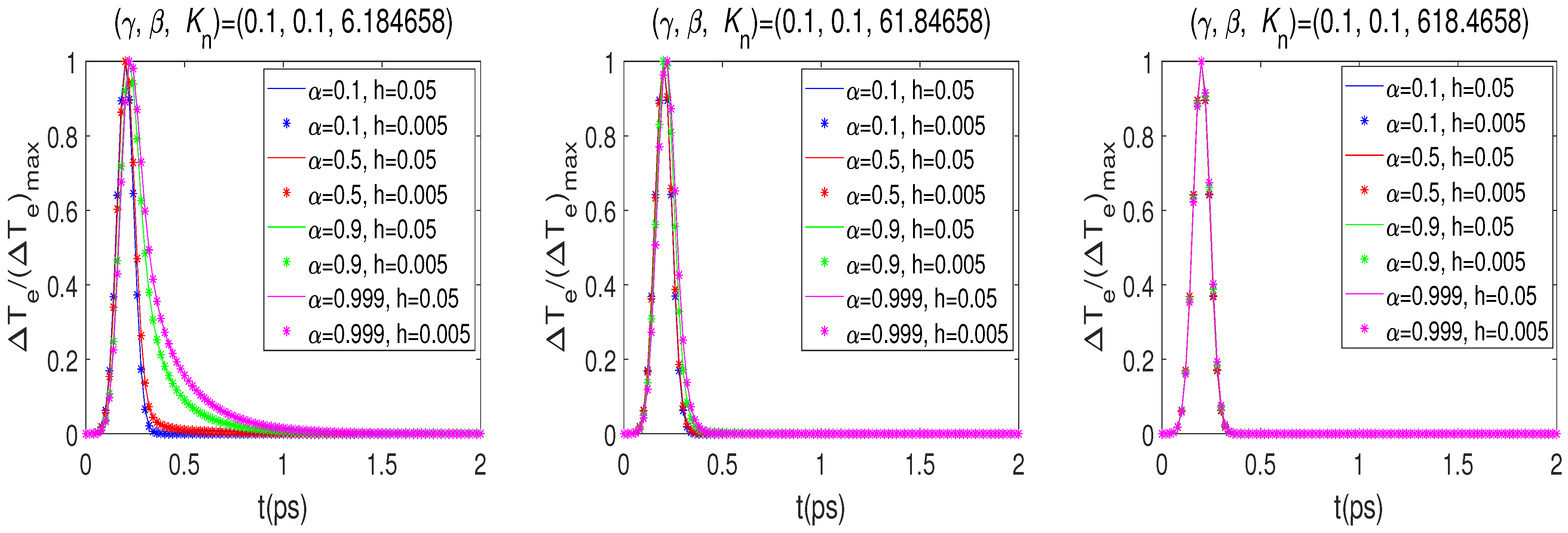
Figure 1.
Changes in electron temperature and various , , and .
Figure 1.
Changes in electron temperature and various , , and .
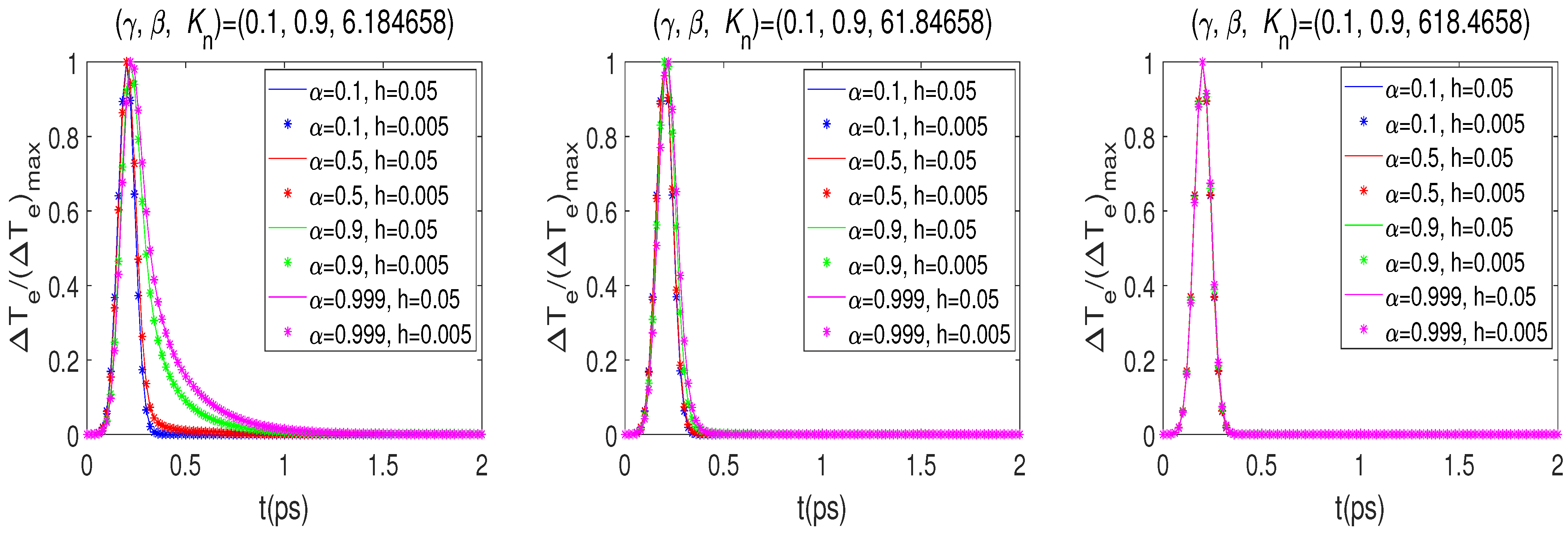
Figure 2.
Changes in electron temperature and various , , and .
Figure 2.
Changes in electron temperature and various , , and .
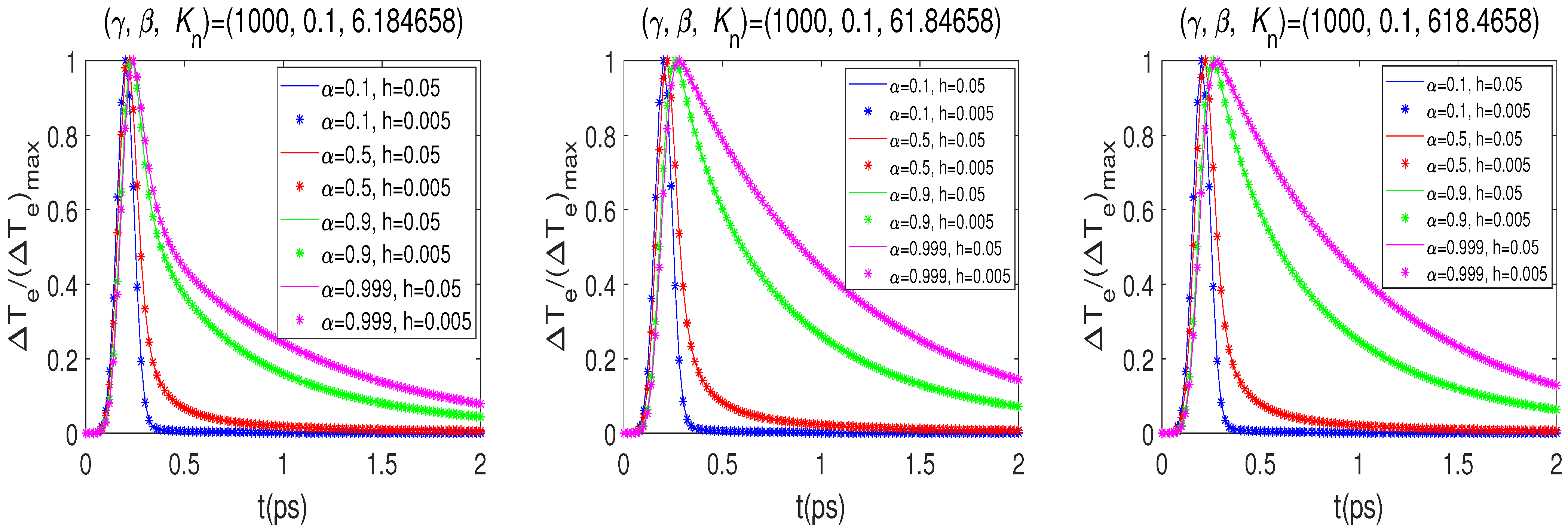
Figure 3.
Changes in electron temperature and various , , and .
Figure 3.
Changes in electron temperature and various , , and .
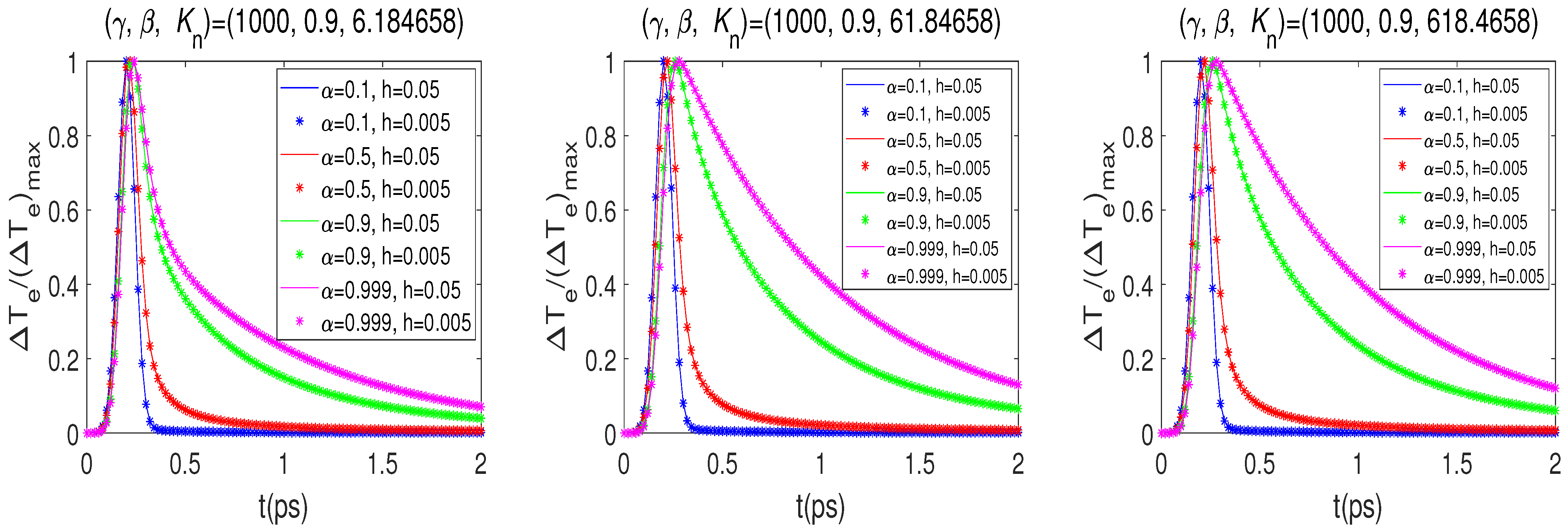
Figure 4.
Changes in electron temperature and various , , and .
Figure 4.
Changes in electron temperature and various , , and .
Figure 5.
Changes in electron temperature and various , , and .
Figure 5.
Changes in electron temperature and various , , and .
Figure 6.
Changes in electron temperature and various , , and .
Figure 6.
Changes in electron temperature and various , , and .
Figure 7.
Changes in electron temperature and various , , and .
Figure 7.
Changes in electron temperature and various , , and .
Figure 8.
Changes in electron temperature and various , , and .
Figure 8.
Changes in electron temperature and various , , and .
Figure 9.
Changes in electron temperature and various , , and .
Figure 9.
Changes in electron temperature and various , , and .
Figure 10.
Changes in electron temperature and various , , and .
Figure 10.
Changes in electron temperature and various , , and .
Figure 11.
Changes in electron temperature and various , , and .
Figure 11.
Changes in electron temperature and various , , and .
Figure 12.
Changes in electron temperature and various , , and .
Figure 12.
Changes in electron temperature and various , , and .
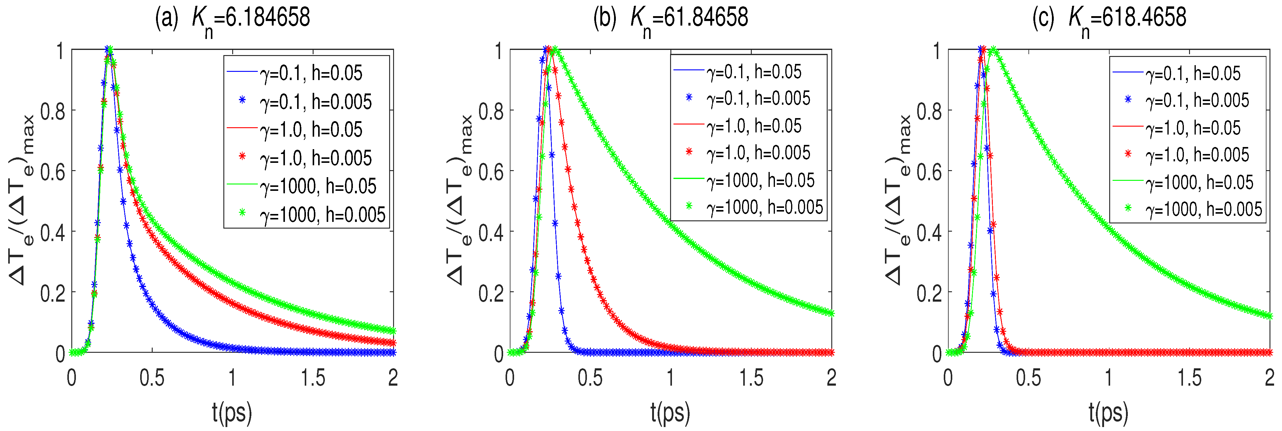
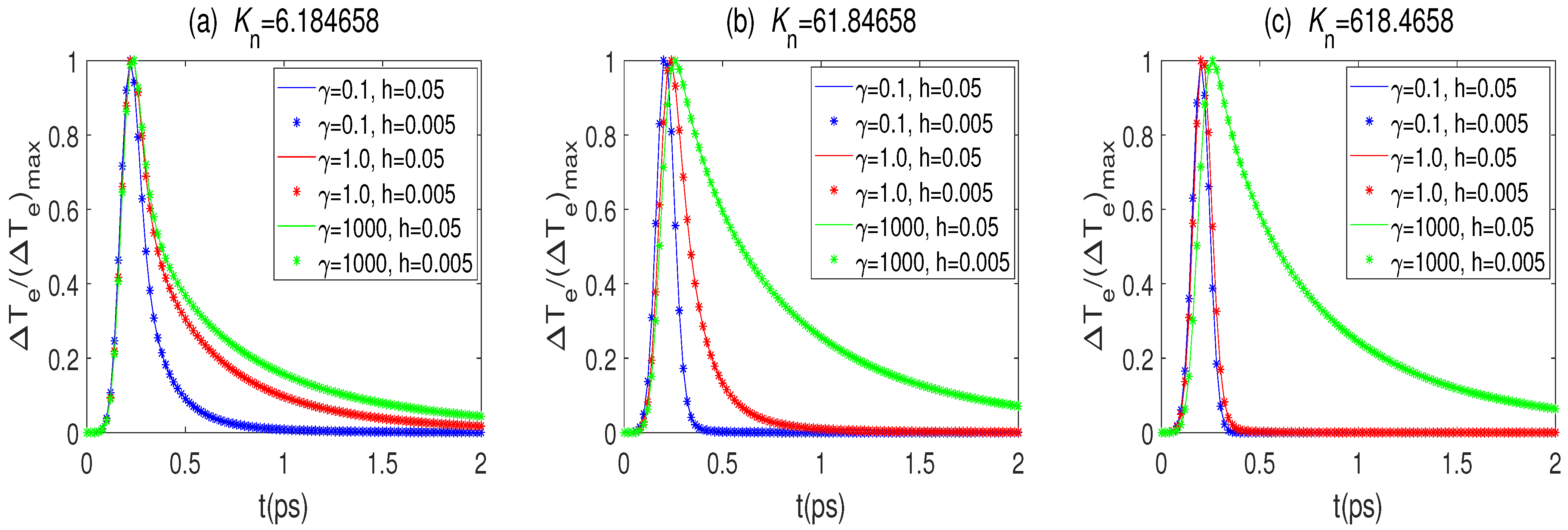
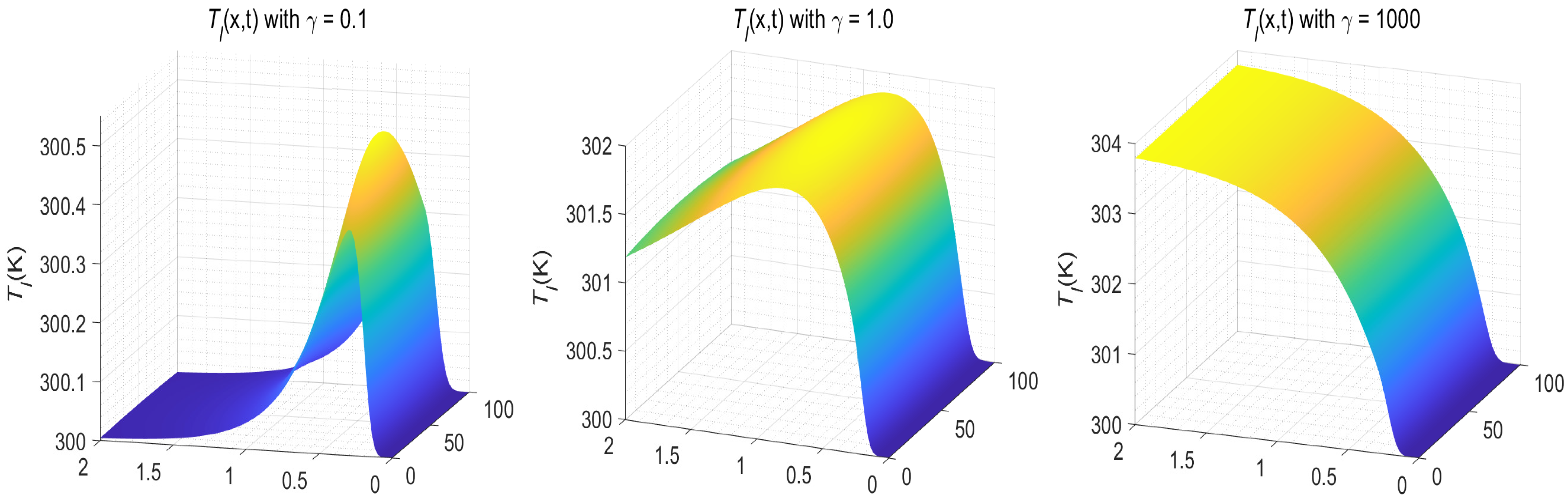
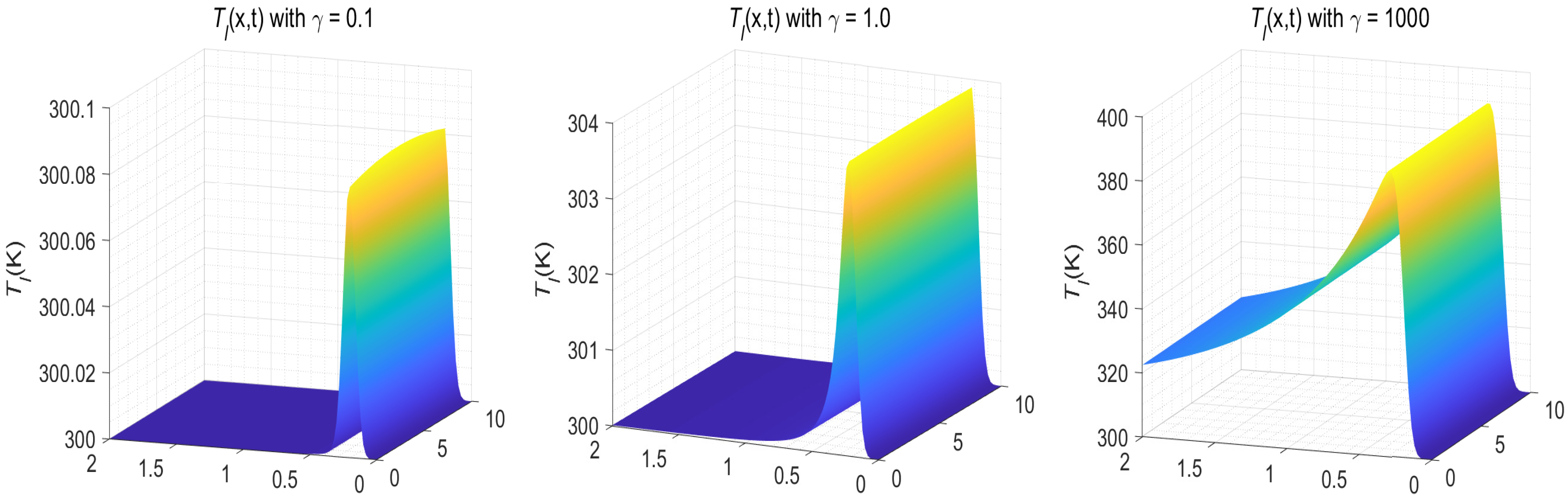
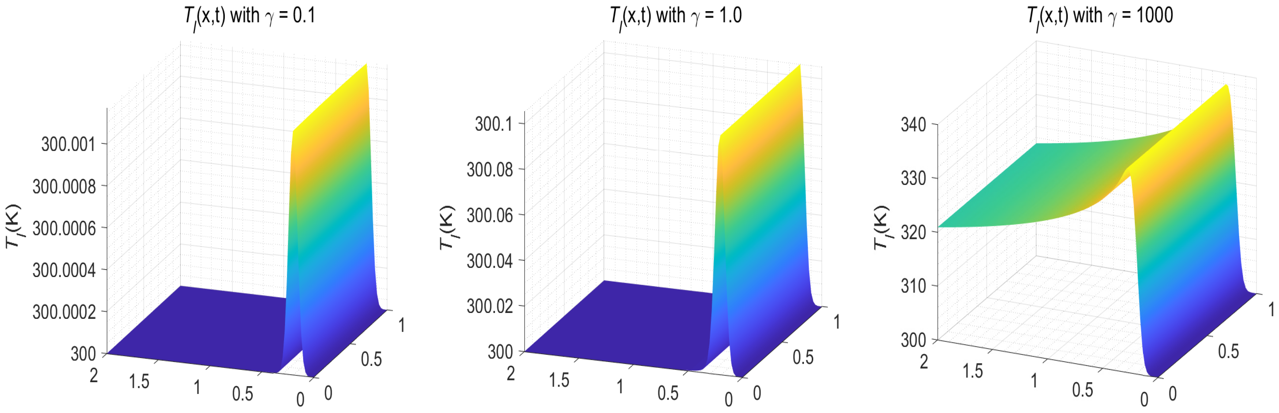
Figure 13.
Temperature distributions of versus with various when , , , and for Example 2.
Figure 13.
Temperature distributions of versus with various when , , , and for Example 2.
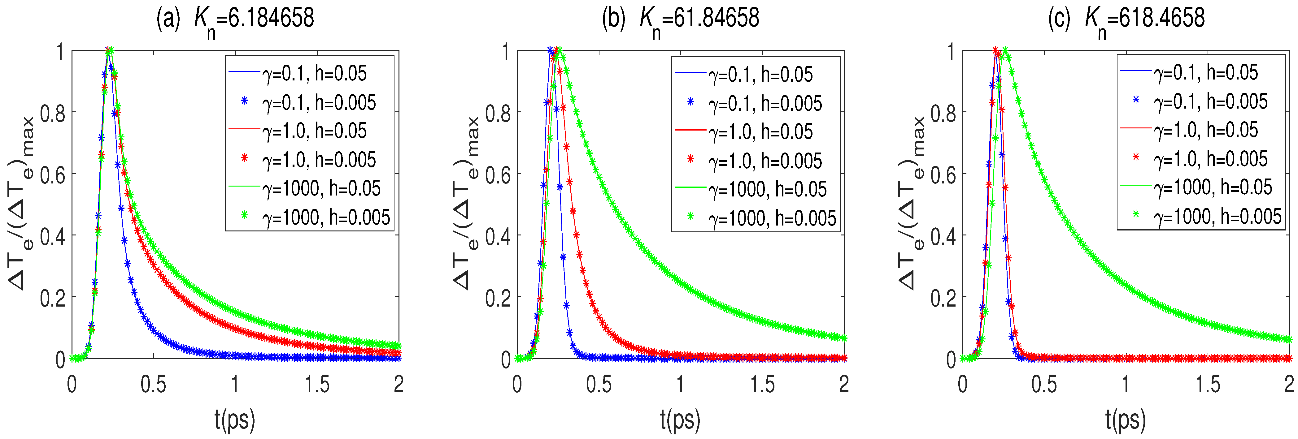
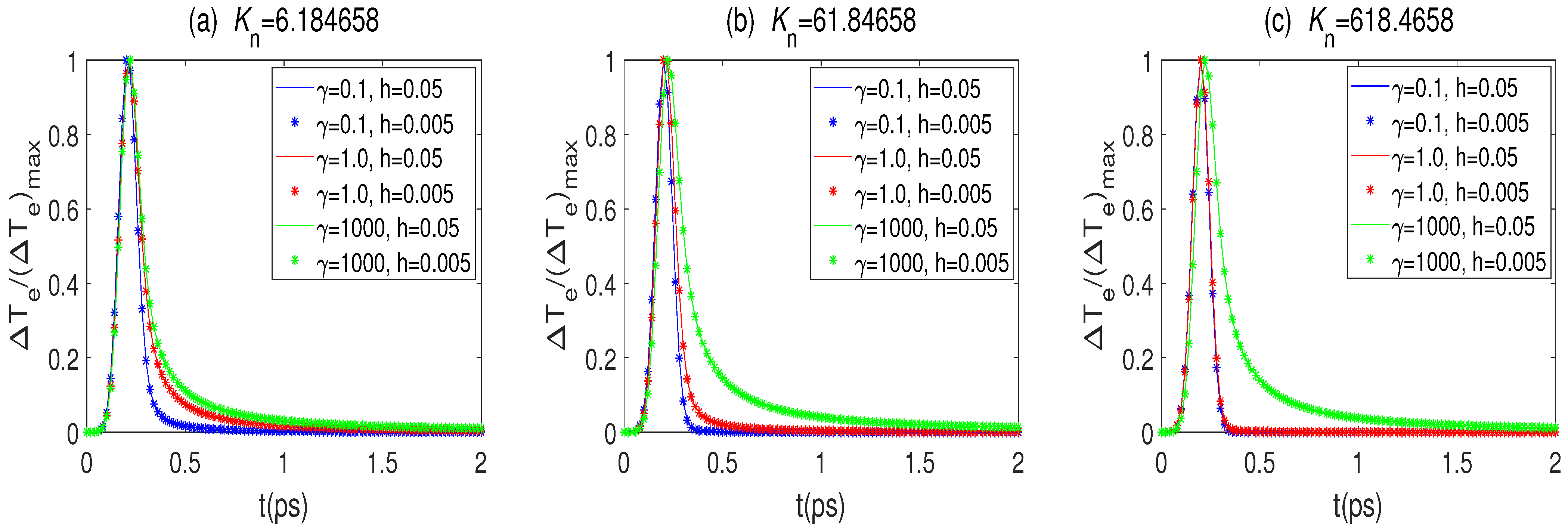
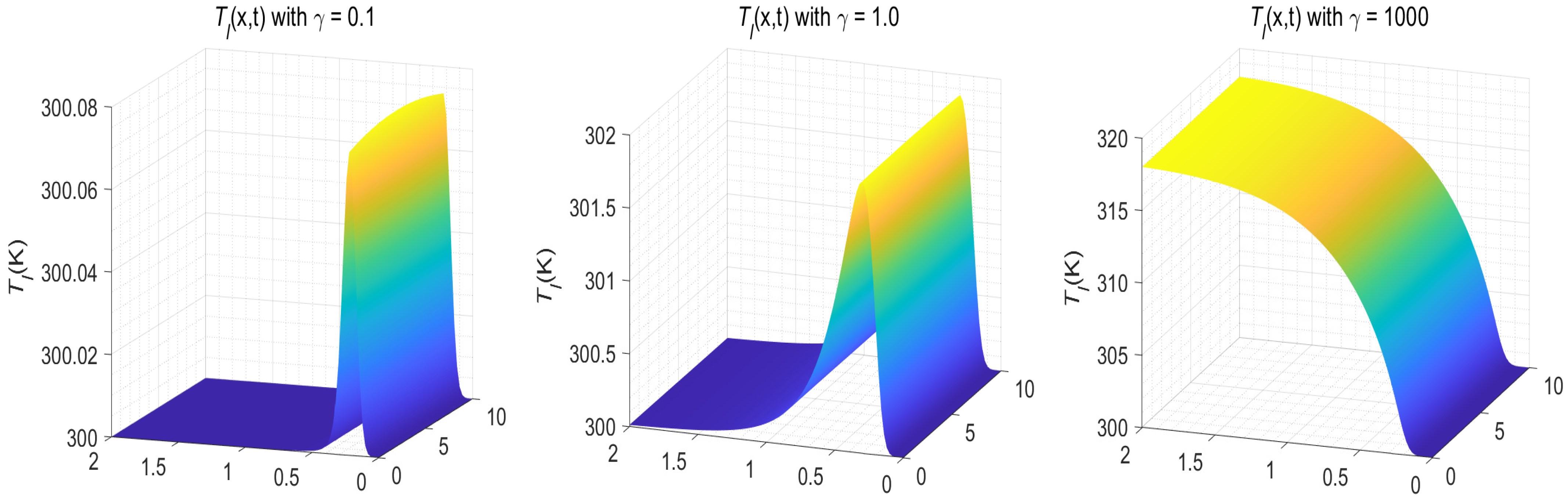
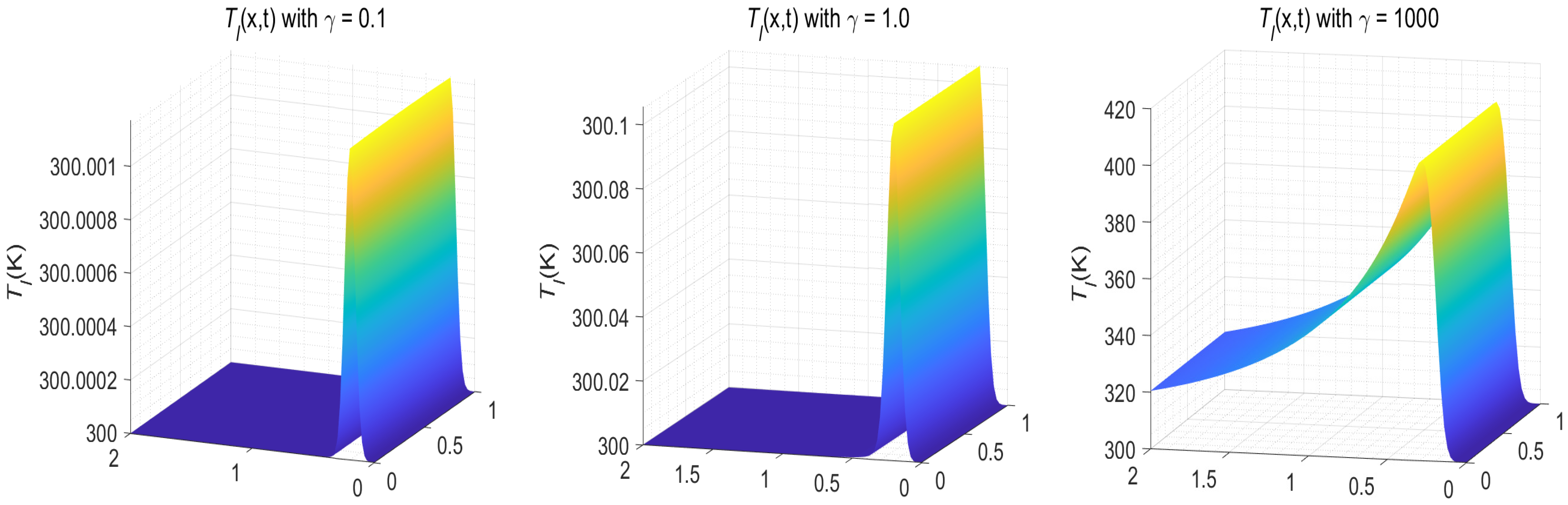
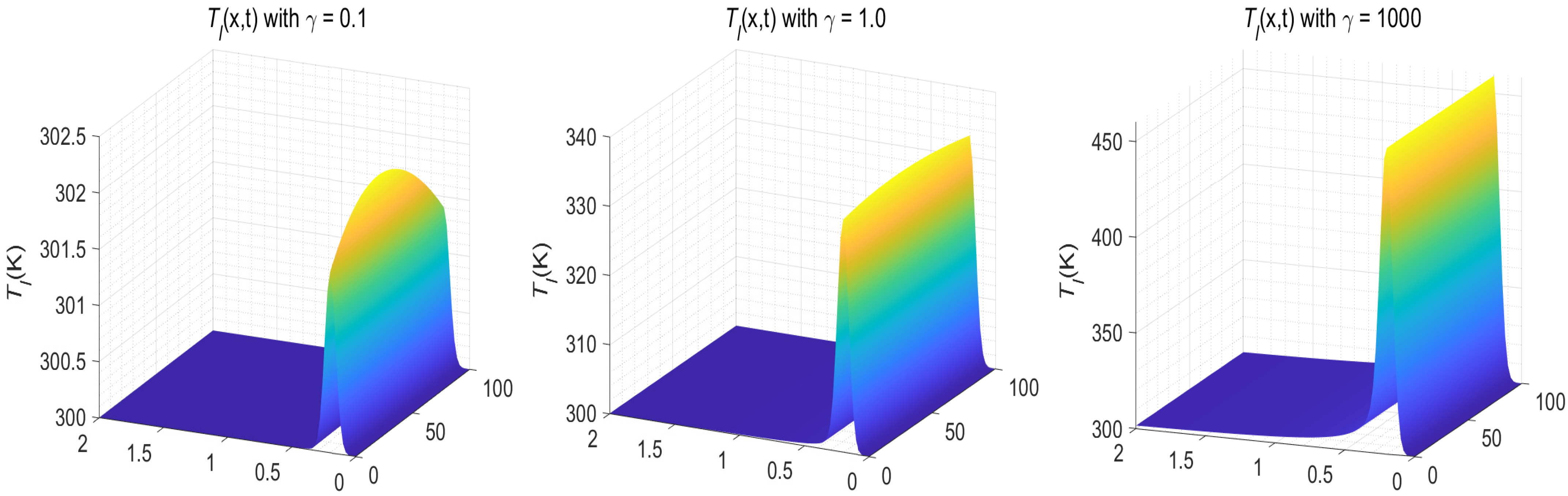
Figure 14.
Temperature distributions of versus with various when , , , and for Example 2.
Figure 14.
Temperature distributions of versus with various when , , , and for Example 2.
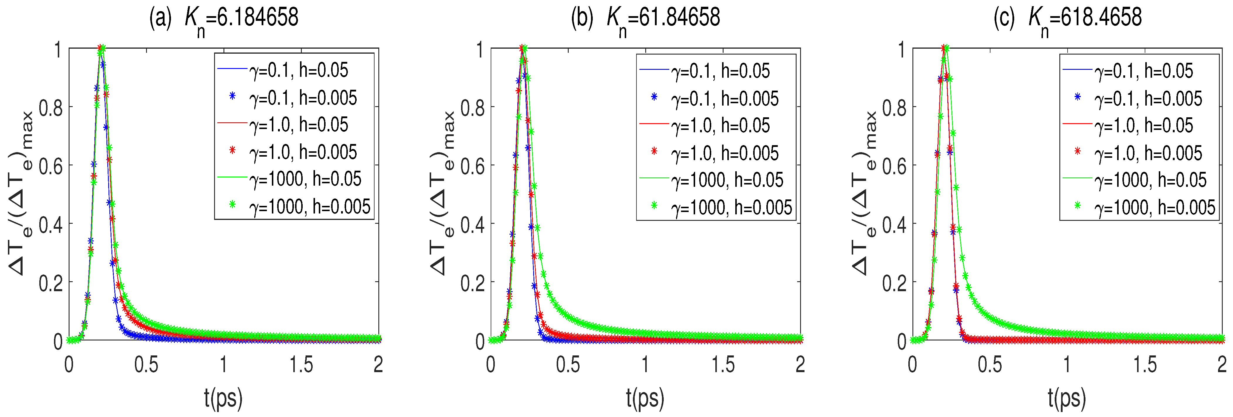
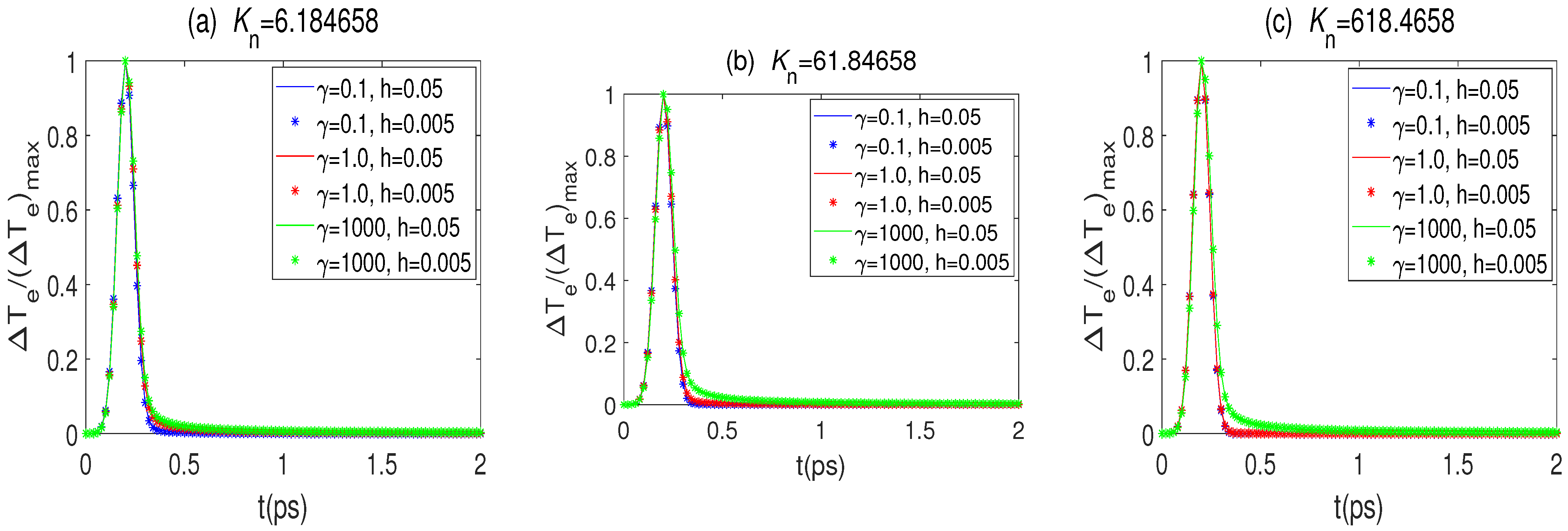
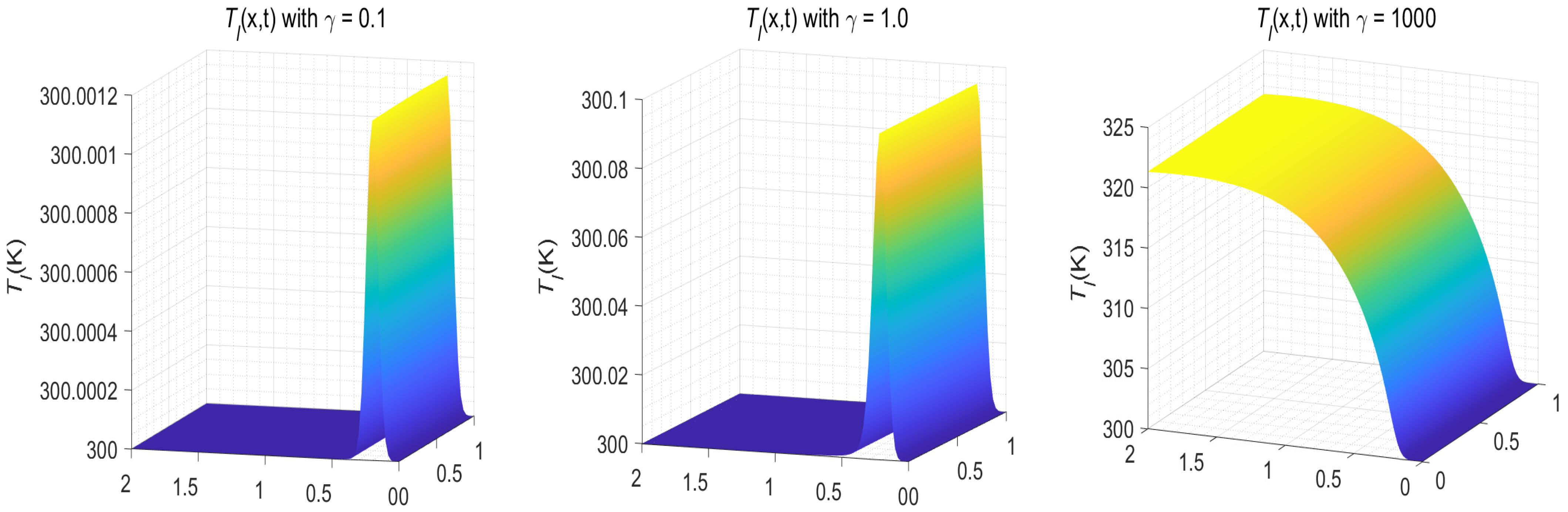
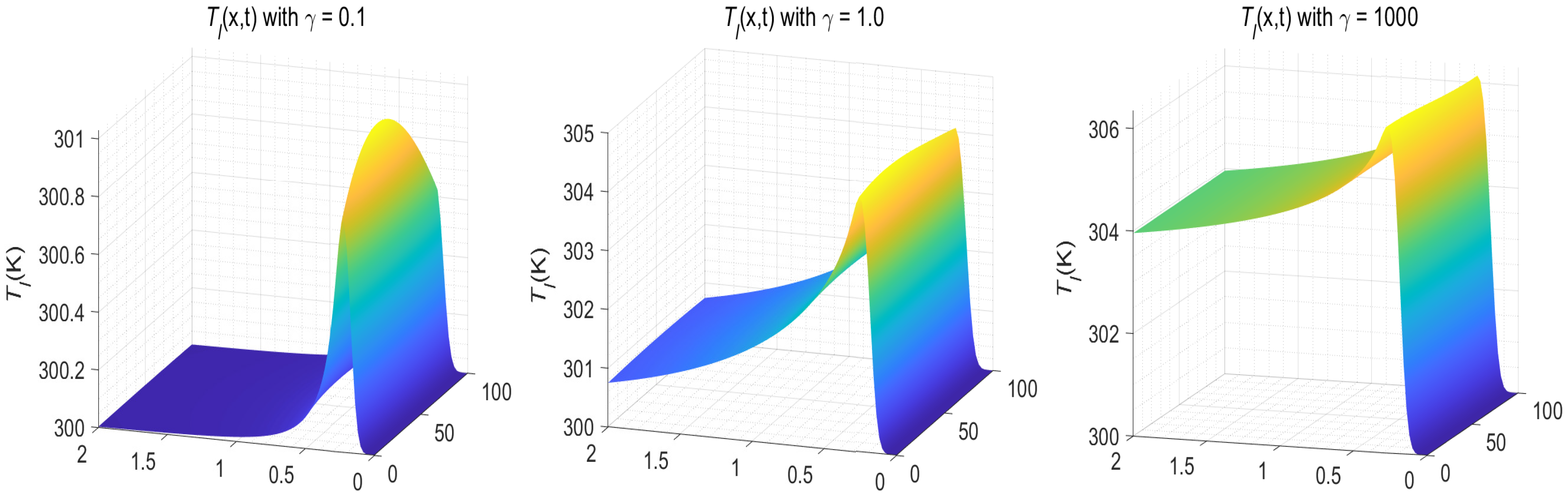
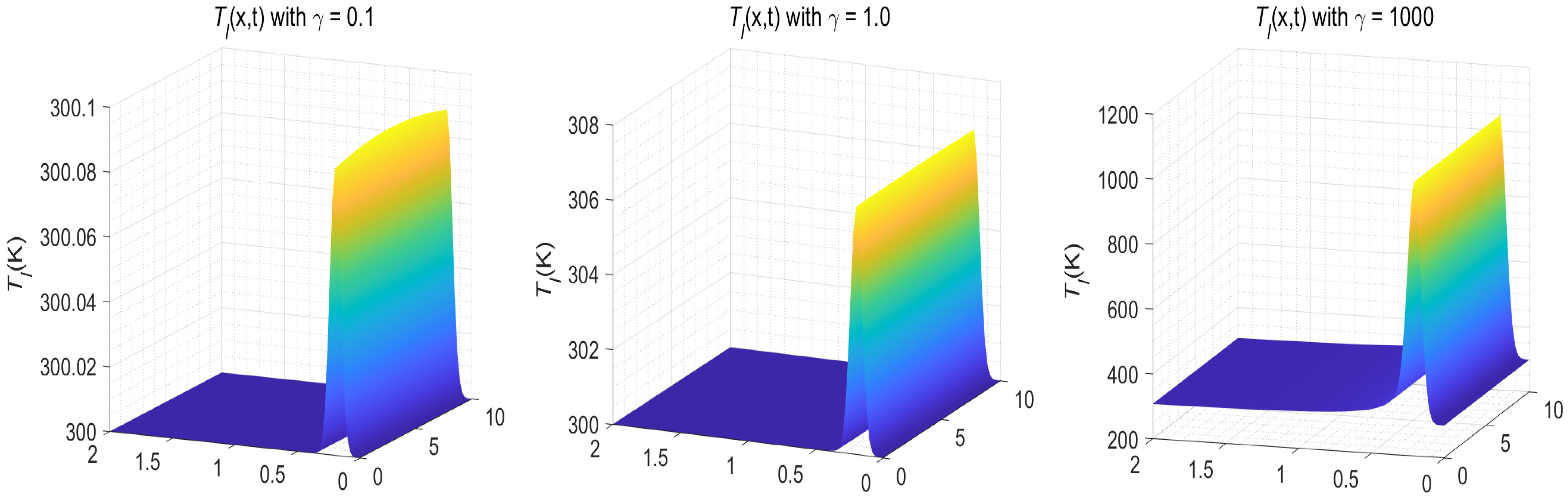
Figure 15.
Temperature distributions of versus with various when , , , and for Example 2.
Figure 15.
Temperature distributions of versus with various when , , , and for Example 2.
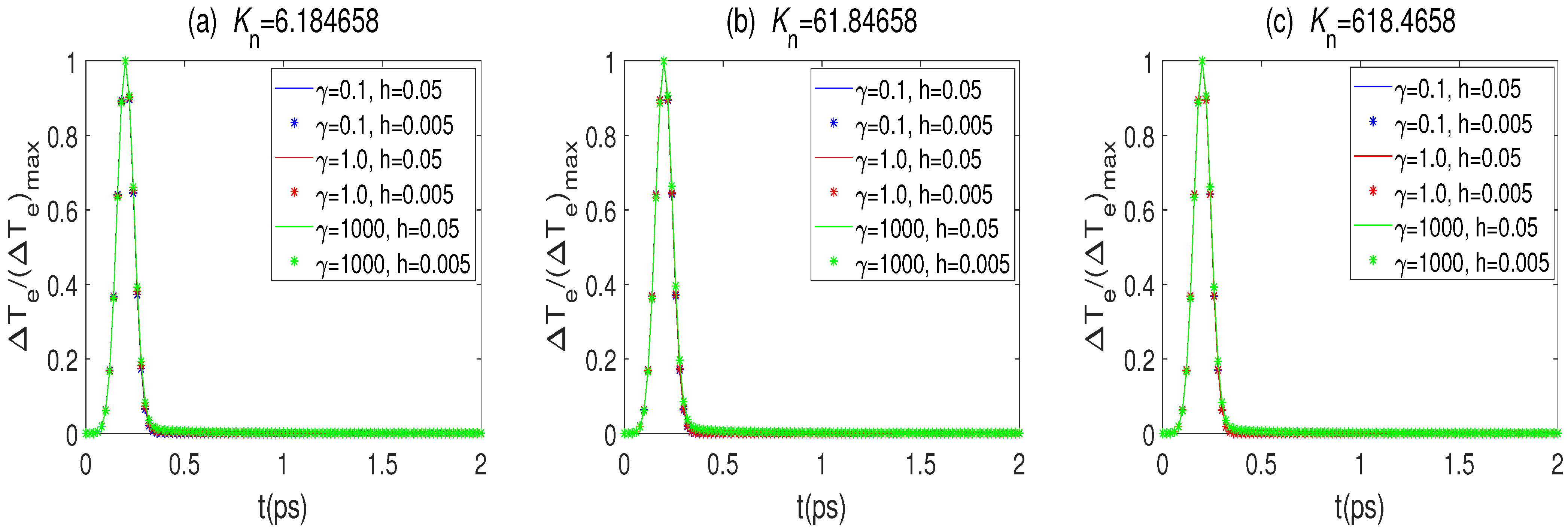
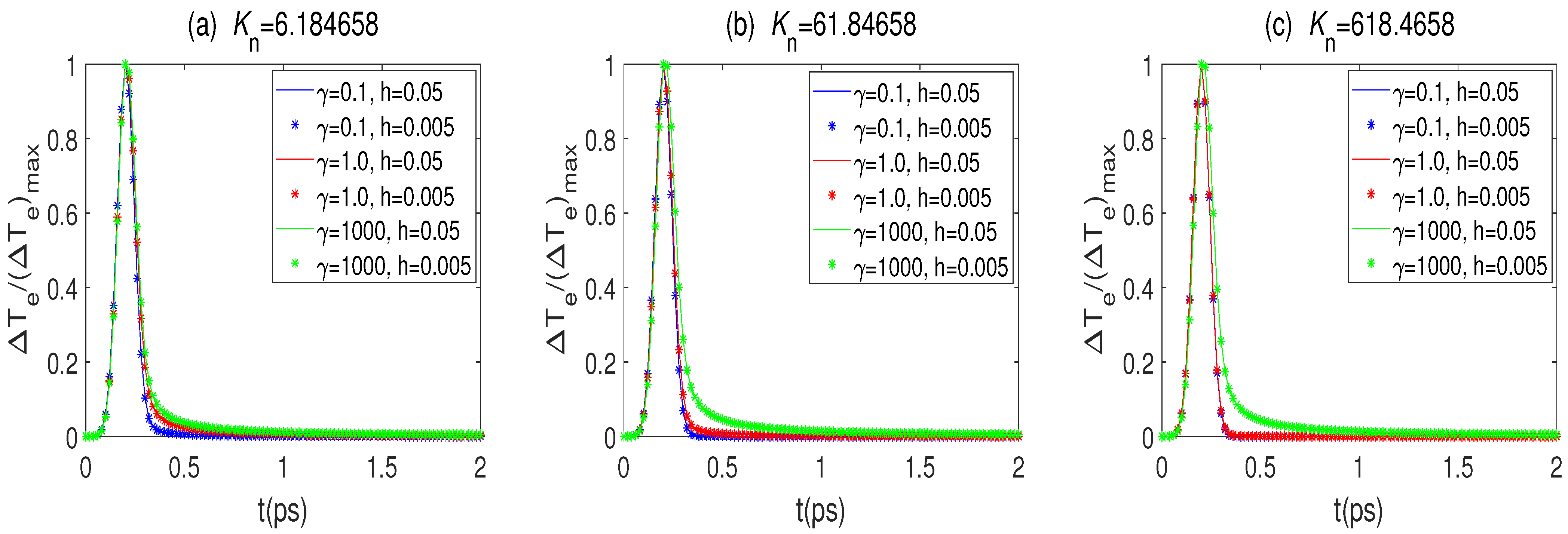
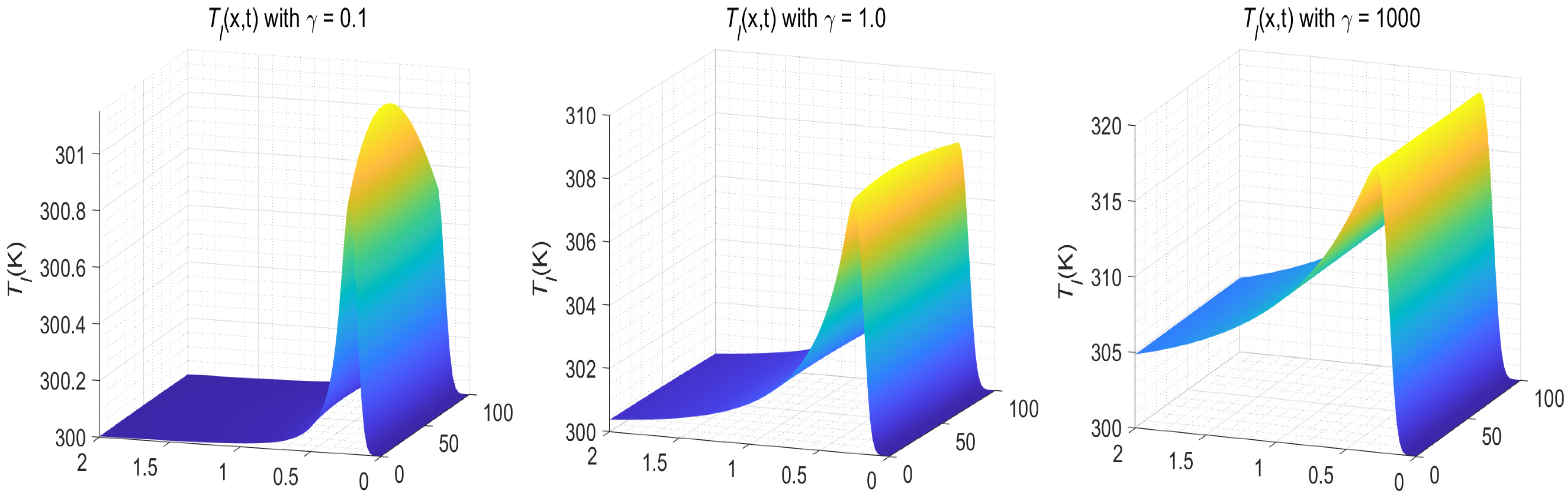
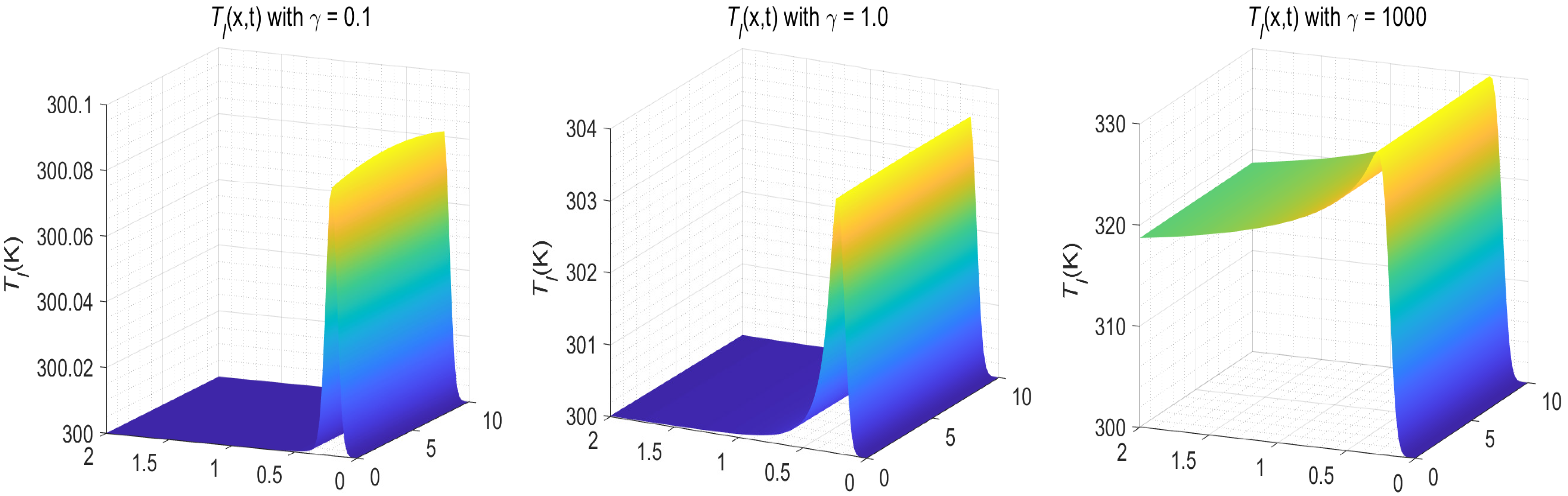
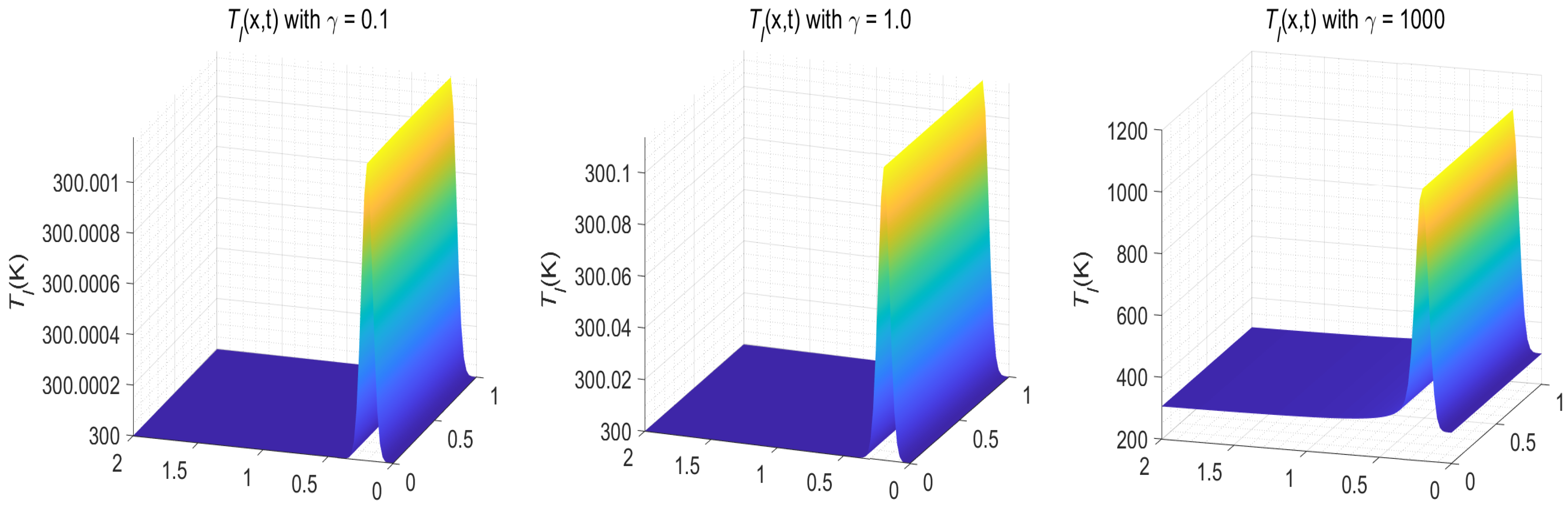
Figure 16.
Temperature distributions of versus with various when , , , and for Example 2.
Figure 16.
Temperature distributions of versus with various when , , , and for Example 2.
Figure 17.
Temperature distributions of versus with various when , , , and for Example 2.
Figure 17.
Temperature distributions of versus with various when , , , and for Example 2.
Figure 18.
Temperature distributions of versus with various when , , , and for Example 2.
Figure 18.
Temperature distributions of versus with various when , , , and for Example 2.
Figure 19.
Temperature distributions of versus with various when , , , and for Example 2.
Figure 19.
Temperature distributions of versus with various when , , , and for Example 2.
Figure 20.
Temperature distributions of versus with various when , , , and for Example 2.
Figure 20.
Temperature distributions of versus with various when , , , and for Example 2.
Figure 21.
Temperature distributions of versus with various when , , , and for Example 2.
Figure 21.
Temperature distributions of versus with various when , , , and for Example 2.
Figure 22.
Temperature distributions of versus with various when , , , and for Example 2.
Figure 22.
Temperature distributions of versus with various when , , , and for Example 2.
Figure 23.
Temperature distributions of versus with various when , , , and for Example 2.
Figure 23.
Temperature distributions of versus with various when , , , and for Example 2.
Figure 24.
Temperature distributions of versus with various when , , , and for Example 2.
Figure 24.
Temperature distributions of versus with various when , , , and for Example 2.
Table 1.
Temporal convergence rate when and for Example 1.
Table 1.
Temporal convergence rate when and for Example 1.
| | | | |
|---|
| | | | | | | |
|---|
| N | | | | | | | | | | | | |
|---|
| 300 | 4.923 | - | 2.997 | - | 6.473 | - | 2.719 | - | 9.130 | - | 1.063 | - |
| 600 | 1.546 | 1.671 | 9.305 | 1.687 | 2.038 | 1.667 | 8.494 | 1.678 | 2.878 | 1.665 | 3.350 | 1.666 |
| 1200 | 4.830 | 1.678 | 2.875 | 1.694 | 6.386 | 1.674 | 2.641 | 1.685 | 9.030 | 1.673 | 1.050 | 1.673 |
| 2400 | 1.503 | 1.684 | 8.852 | 1.700 | 1.993 | 1.680 | 8.180 | 1.691 | 2.817 | 1.680 | 3.275 | 1.681 |
Table 2.
Temporal convergence rate when and for Example 1.
Table 2.
Temporal convergence rate when and for Example 1.
| | | | |
|---|
| | | | | | | |
|---|
| N | | | | | | | | | | | | |
|---|
| 300 | 7.702 | - | 3.586 | - | 1.114 | - | 3.885 | - | 1.730 | - | 1.984 | - |
| 600 | 3.132 | 1.298 | 1.443 | 1.313 | 4.538 | 1.296 | 1.573 | 1.304 | 7.046 | 1.296 | 8.080 | 1.296 |
| 1200 | 1.272 | 1.300 | 5.816 | 1.311 | 1.846 | 1.298 | 6.369 | 1.304 | 2.867 | 1.297 | 3.287 | 1.298 |
| 2400 | 5.167 | 1.300 | 2.346 | 1.309 | 7.502 | 1.299 | 2.579 | 1.304 | 1.166 | 1.298 | 1.336 | 1.299 |
Table 3.
Temporal convergence rate when and for Example 1.
Table 3.
Temporal convergence rate when and for Example 1.
| | | | |
|---|
| | | | | | | |
|---|
| N | | | | | | | | | | | | |
|---|
| 300 | 2.427 | - | 1.771 | - | 3.026 | - | 1.457 | - | 4.236 | - | 4.944 | - |
| 600 | 8.659 | 1.487 | 6.320 | 1.486 | 1.079 | 1.487 | 5.199 | 1.486 | 1.511 | 1.488 | 1.763 | 1.487 |
| 1200 | 3.080 | 1.491 | 2.250 | 1.490 | 3.840 | 1.491 | 1.850 | 1.490 | 5.373 | 1.491 | 6.274 | 1.491 |
| 2400 | 1.094 | 1.494 | 7.991 | 1.493 | 1.364 | 1.494 | 6.572 | 1.493 | 1.907 | 1.495 | 2.227 | 1.495 |
Table 4.
Spatial convergence rate when and for Example 1.
Table 4.
Spatial convergence rate when and for Example 1.
| | | | |
|---|
| | | | | | | |
|---|
| M | | | | | | | | | | | | |
|---|
| 30 | 2.783 | - | 1.647 | - | 5.404 | - | 1.705 | - | 5.333 | - | 6.034 | - |
| 60 | 7.297 | 1.932 | 4.169 | 1.982 | 1.352 | 1.999 | 4.260 | 2.001 | 1.333 | 2.000 | 1.508 | 2.000 |
| 120 | 1.848 | 1.982 | 1.045 | 1.996 | 3.380 | 2.000 | 1.065 | 2.000 | 3.332 | 2.000 | 3.770 | 2.000 |
| 240 | 4.634 | 1.995 | 2.614 | 1.999 | 8.449 | 2.000 | 2.662 | 2.000 | 8.330 | 2.000 | 9.426 | 2.000 |
Table 5.
Spatial convergence rate when and for Example 1.
Table 5.
Spatial convergence rate when and for Example 1.
| | | | |
|---|
| | | | | | | |
|---|
| M | | | | | | | | | | | | |
|---|
| 30 | 2.518 | - | 1.511 | - | 4.928 | - | 1.485 | - | 4.878 | - | 5.396 | - |
| 60 | 6.753 | 1.899 | 3.849 | 1.974 | 1.233 | 1.999 | 3.710 | 2.001 | 1.219 | 2.000 | 1.349 | 2.000 |
| 120 | 1.721 | 1.972 | 9.656 | 1.995 | 3.084 | 2.000 | 9.273 | 2.000 | 3.048 | 2.000 | 3.371 | 2.000 |
| 240 | 4.323 | 1.993 | 2.416 | 1.999 | 7.710 | 2.000 | 2.318 | 2.000 | 7.621 | 2.000 | 8.429 | 2.000 |
Table 6.
Spatial convergence rate when and for Example 1.
Table 6.
Spatial convergence rate when and for Example 1.
| | | | |
|---|
| | | | | | | |
|---|
| M | | | | | | | | | | | | |
|---|
| 30 | 3.105 | - | 1.512 | - | 5.542 | - | 1.490 | - | 5.125 | - | 5.438 | - |
| 60 | 8.237 | 1.915 | 3.851 | 1.973 | 1.386 | 1.999 | 3.724 | 2.001 | 1.281 | 2.000 | 1.359 | 2.000 |
| 120 | 2.093 | 1.977 | 9.661 | 1.995 | 3.467 | 2.000 | 9.308 | 2.000 | 3.202 | 2.000 | 3.398 | 2.000 |
| 240 | 5.253 | 1.994 | 2.417 | 1.999 | 8.667 | 2.000 | 2.327 | 2.000 | 8.006 | 2.000 | 8.494 | 2.000 |
Table 7.
Thermal properties of gold film.
Table 7.
Thermal properties of gold film.
| | | | | |
|---|
| 300 | 315 | | | | 8.5 |
Table 8.
Temporal convergence rate when and for Example 2.
Table 8.
Temporal convergence rate when and for Example 2.
| | | | |
|---|
| | | | | | | |
|---|
| N | | | | | | | | | | | | |
|---|
| 50 | 5.891 | - | 8.810 | - | 5.632 | - | 7.573 | - | 1.035 | - | 1.607 | - |
| 100 | 3.033 | 0.958 | 4.123 | 1.096 | 2.751 | 1.034 | 3.542 | 1.096 | 4.404 | 1.232 | 7.803 | 1.042 |
| 200 | 1.489 | 1.026 | 1.926 | 1.098 | 1.315 | 1.064 | 1.654 | 1.099 | 1.980 | 1.153 | 3.725 | 1.067 |
| 400 | 7.146 | 1.059 | 8.987 | 1.099 | 6.218 | 1.081 | 7.715 | 1.100 | 8.915 | 1.151 | 1.753 | 1.087 |
| 800 | 3.387 | 1.077 | 4.193 | 1.100 | 2.924 | 1.089 | 3.601 | 1.099 | 3.769 | 1.242 | 8.089 | 1.116 |
| 1600 | 1.595 | 1.087 | 1.957 | 1.100 | 1.372 | 1.092 | 1.682 | 1.098 | 1.832 | 1.040 | 3.788 | 1.094 |
Table 9.
Spatial convergence rate when 50,000 and for Example 2.
Table 9.
Spatial convergence rate when 50,000 and for Example 2.
| | | | |
|---|
| | | | | | | |
|---|
| M | | | | | | | | | | | | |
|---|
| 5 | 2.376 | - | 1.231 | - | 9.452 | - | 4.695 | - | 3.154 | - | 5.711 | - |
| 10 | 6.087 | 1.965 | 3.157 | 1.963 | 2.364 | 2.000 | 1.174 | 2.000 | 7.891 | 1.999 | 1.435 | 1.993 |
| 20 | 1.531 | 1.991 | 7.945 | 1.990 | 5.909 | 2.000 | 2.935 | 2.000 | 1.982 | 1.994 | 3.775 | 1.927 |
| 40 | 3.834 | 1.998 | 1.989 | 1.998 | 1.477 | 2.000 | 7.337 | 2.000 | 5.211 | 1.927 | 9.411 | 2.004 |
Table 10.
with different , , and () for Example 2.
Table 10.
with different , , and () for Example 2.
| | | | |
|---|
| 0.1 | 757.42 | 651.67 | 353.96 |
| | 1.0 | 984.85 | 1598.12 | 761.43 |
| | 1000 | 1025.05 | 2172.28 | 2757.17 |
| 0.1 | 841.14 | 663.45 | 354.14 |
| | 1.0 | 1150.01 | 1937.69 | 776.67 |
| | 1000 | 1214.15 | 2925.78 | 3740.83 |
| 0.1 | 1113.91 | 699.34 | 354.51 |
| | 1.0 | 2171.79 | 3086.01 | 822.71 |
| | 1000 | 2550.34 | 8756.41 | 11,241.11 |
| 0.1 | 1213.70 | 706.58 | 354.61 |
| | 1.0 | 2977.20 | 3513.14 | 832.01 |
| | 1000 | 3943.96 | 15,031.85 | 18,973.40 |
Table 11.
with different , , and () for Example 2.
Table 11.
with different , , and () for Example 2.
| | | | |
|---|
| 0.10 | 841.18 | 663.45 | 354.14 |
| | 1.0 | 1150.47 | 1937.89 | 776.68 |
| | 1000 | 1215.44 | 2933.69 | 3750.36 |
| 0.10 | 988.45 | 688.67 | 354.37 |
| | 1.0 | 1642.03 | 2613.69 | 809.00 |
| | 1000 | 1799.97 | 5331.86 | 6855.04 |
| 0.10 | 1057.69 | 695.02 | 354.45 |
| | 1.0 | 1918.58 | 2839.52 | 817.16 |
| | 1000 | 2174.02 | 6990.35 | 8995.89 |
| 0.10 | 1113.93 | 699.34 | 354.51 |
| | 1.0 | 2173.07 | 3086.08 | 822.71 |
| | 1000 | 2554.85 | 8777.67 | 11,266.18 |
Table 12.
with different , , and () for Example 2.
Table 12.
with different , , and () for Example 2.
| | | | |
|---|
| 0.1 | 1181.55 | 704.33 | 354.58 |
| | 1.0 | 2670.49 | 3376.66 | 829.12 |
| | 1000 | 3302.87 | 12,045.75 | 15,400.19 |
| 0.1 | 1181.47 | 704.33 | 354.58 |
| | 1.0 | 2668.95 | 3376.35 | 829.12 |
| | 1000 | 3299.93 | 12,031.88 | 15,382.99 |
| 0.1 | 1153.86 | 702.30 | 354.55 |
| | 1.0 | 2450.32 | 3258.21 | 826.52 |
| | 1000 | 2941.02 | 10,362.09 | 13,284.13 |
| 0.1 | 1153.83 | 702.30 | 354.55 |
| | 1.0 | 2448.84 | 3258.11 | 826.52 |
| | 1000 | 2937.51 | 10,345.52 | 13,264.02 |


