1. Introduction
Mechanical oscillators play a vital role in many fields, such as engineering [
1], lattice dynamics [
2], and biology [
3]. Due to the changes in geometric configuration, strong irrational nonlinearities occur in many oscillators [
4,
5,
6]. A typical example is the smooth and discontinuous (SD) oscillator proposed by Cao et al. [
7,
8]. It is geometrically nonlinear, with an irrationally nonlinear restoring force. Whether it is smooth or discontinuous depends on the value of its smoothness parameter. Representing the snap-through truss system, this oscillator has been found to exhibit a large variety and complexity of responses and phenomena [
9,
10,
11], thus receiving much attention in recent years.
Many studies have been conducted to provide a fundamental basis for understanding the dynamics of the SD oscillator. Tian et al. [
12] investigated the universal unfolding for codimension-two bifurcation near the equilibria of the SD oscillator, such as pitchfork, Hopf and double Hopf, and double-connected homoclinic and closed-orbit bifurcations. Li et al. [
13] obtained periodic solutions of the SD oscillator by applying the four-dimensional averaging method and the complete Jacobian elliptic integrals [
13]. On this basis, the stick–slip vibrations and complex equilibrium bifurcations of a self-excited SD oscillator with Coulomb friction were discussed [
14]. Santhosh et al. [
15] carried out the frequency domain analysis of a harmonically excited SD oscillator semi-analytically and found that saddle-node bifurcation leads to jumping phenomena and symmetry-breaking bifurcations. Chen et al. [
16] derived all possible bifurcations of the SD oscillatory system, including degenerate Hopf, homoclinic, double limit cycle, Bautin, and Bogdanov–Takens bifurcations. In terms of the stochastic case, Yue et al. [
17] studied the stochastic bifurcations of the SD oscillator with additive and/or multiplicative bounded noises by using the generalized cell mapping method and digraph analysis algorithm. Considering delayed displacement and velocity feedback control, Yang and Cao [
18] analyzed the primary resonance and the noise-induced stochastic resonance of a quasi-zero-stiffness SD oscillator via the average method.
In engineering practice, the SD oscillator has been utilized for vibration absorption and vibration energy harvesting. For the former purpose, Hao and Cao [
19] employed the SD oscillatory system with a stable-quasi-zero-stiffness characteristic as a vibration isolator. For the latter, Yang et al. [
20] proposed an electromagnetic vibration energy harvester based on the SD oscillator and driven by stochastic environmental fluctuation. Zhang et al. [
21] applied the SD oscillator in designing an electromagnetic bistable vibration energy harvester with an elastic boundary and experimentally verified its higher probability for inducing favorable inter-well responses than normal energy harvesters.
Up to now, studies on the SD oscillator have shown that multistability is common in this type of oscillatory system. As it is well known, this initial sensitive dynamical behavior is a double-edged sword in engineering applications: it is unwanted for achieving globally stable mechanical vibration but helpful for achieving desired deformations with small energy input. For instance, by making use of the multistability characteristics of some types of energy harvesters, better energy harvesting performance can be achieved due to the absence of the requirement for a constant supply of energy but with a small perturbation of the initial conditions. Therefore, extending the study on the initial conditions for jumps among the multiple responses of the SD oscillator is essential for its practical applications. Currently, research on the initial conditions is still very limited. Most of the discussions on the multistability of this oscillator focus on the mechanism of multistability triggered by system parameters.
Based on the above statement, the goal of this study is to present the mechanism of jump among the coexisting attractors of the SD oscillator analytically and to classify the fractal basins of attraction of the multiple attractors quantitatively. This paper is organized as follows. In
Section 2, the unperturbed dynamics of the presented archetypal dynamical model are discussed. In
Section 3, the amplitude–frequency characteristics of the steady solutions of the dimensionless system are derived. In
Section 4, numerical explorations are performed to verify the validity of the analytical prediction; meanwhile, the basins of attraction of the coexisting attractors are presented. Some conclusions are drawn thereafter.
2. Dynamical Model and Unperturbed Dynamics
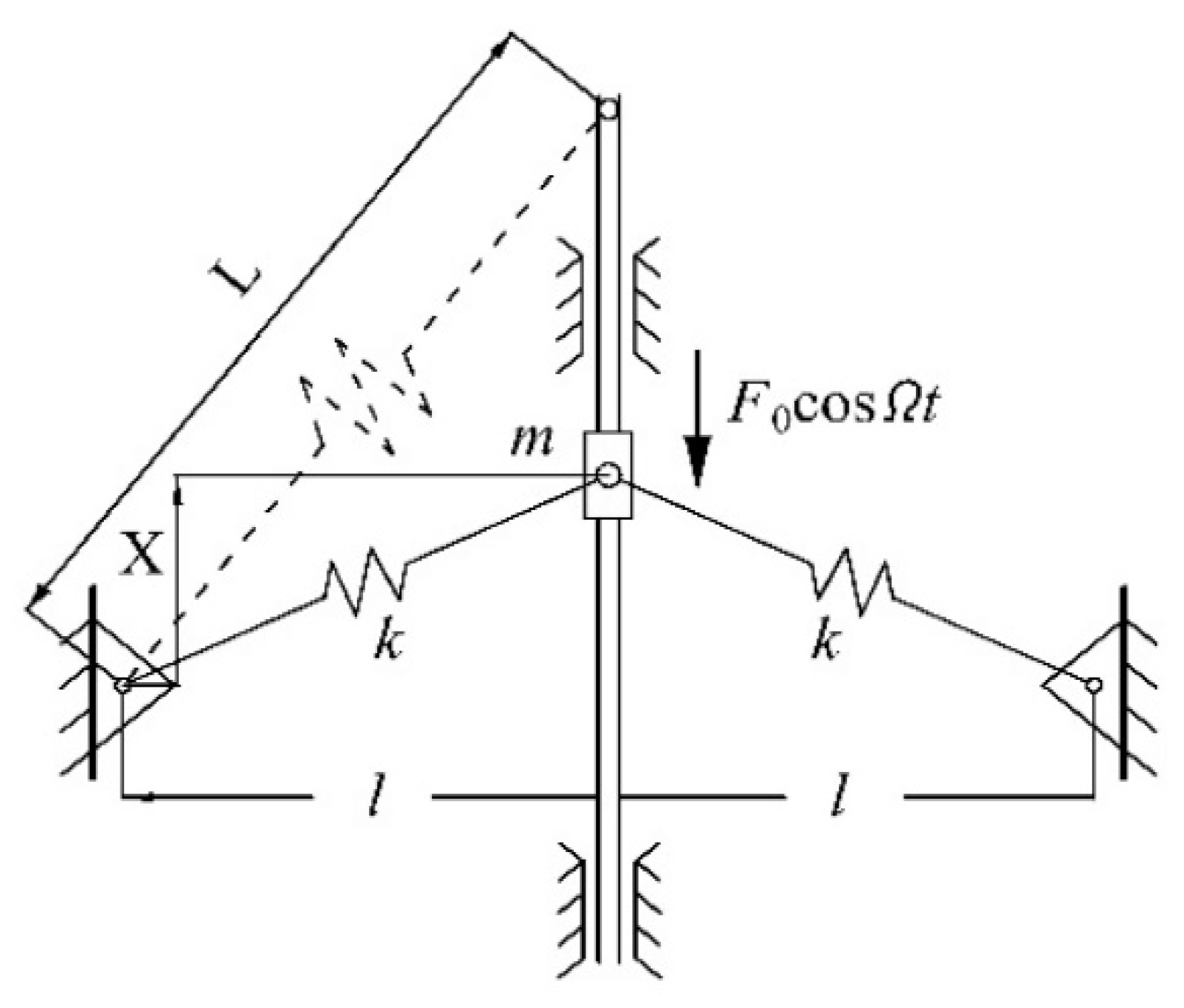
The harmonically excited smooth and discontinuous (SD) oscillator can be represented geometrically as a conventional linear mass–spring–damper system subject to harmonic excitation, as shown in
Figure 1. The loaded mass
m is attached to two springs pinned to rigid supports on the horizontal plane. It is also subjected to the actions of the harmonic-driven force and the viscous damping force. Since the motion of the mass is in the X direction, applying the equation of motion, we have
Here,
X represents the displacement of the mass,
k is the linear stiffness of each spring,
L is the unstretched length of each spring,
l is the half-distance between the pivots of the inclined springs, and
c is the damping coefficient of the viscous damper.
F0 and Ω are the amplitude and frequency of the harmonically excited driven force, respectively. As can be seen in Equation (1), due to the geometric configuration, the resultant of the restoring resistances of the two springs is strongly and irrationally nonlinear even though each spring has a linear stiffness. If we let
we rewrite system (1) as the following dimensionless system:
System (3) is smooth when
. When
, it becomes a discontinuous system given by
Since the distance
l in
Figure 1 is positive, we have
and a smooth system (3). The unperturbed system of system (3) is
Note that the number, position, and stability of its equilibria are determined by the value of the smoothness parameter
. For
, there are three equilibria, i.e., a saddle point
and two centers
where
. For
, there is only one equilibrium
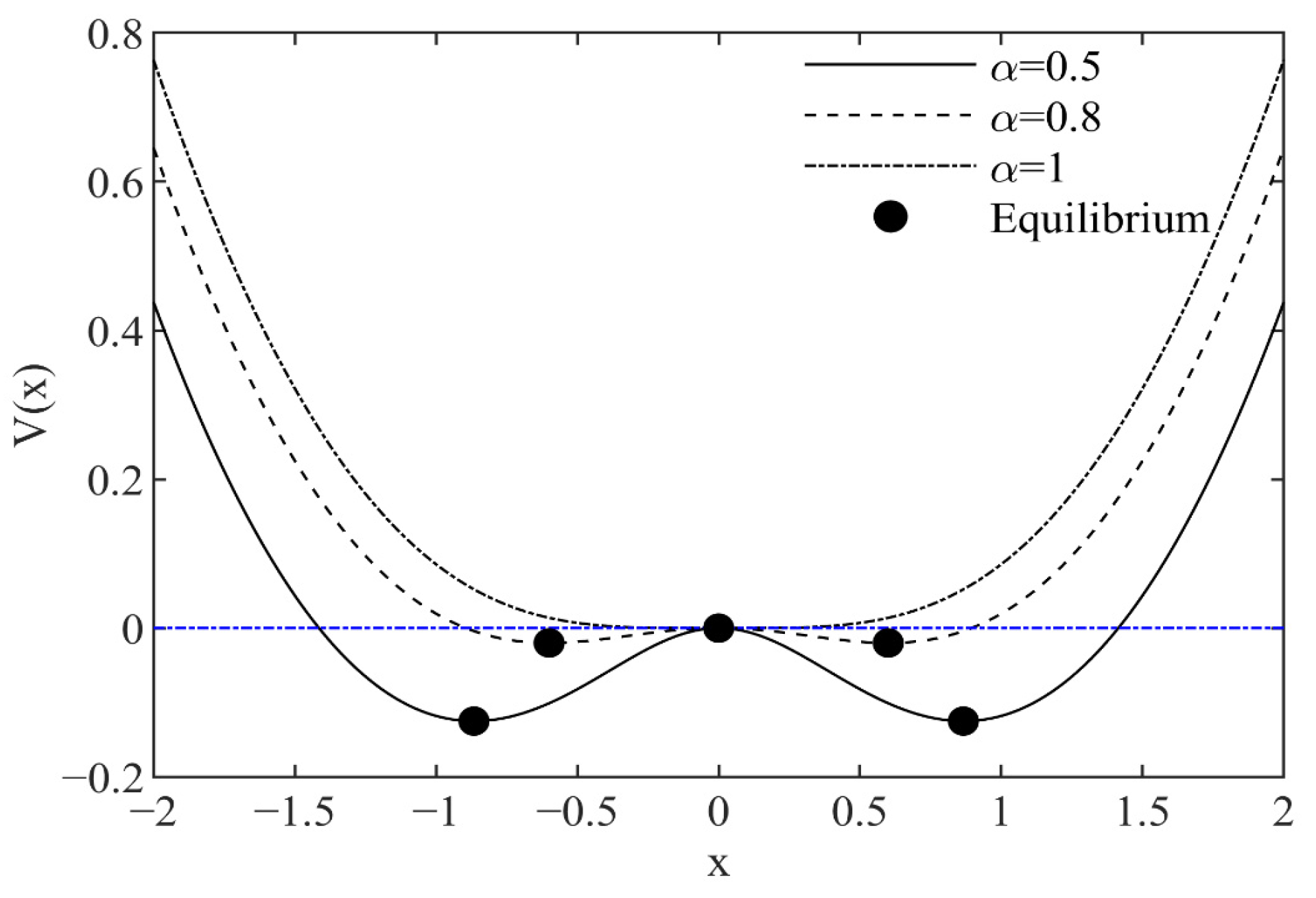
. Equation (5) is a Hamilton system with the Hamiltonian
and the function of potential energy
in the following form:
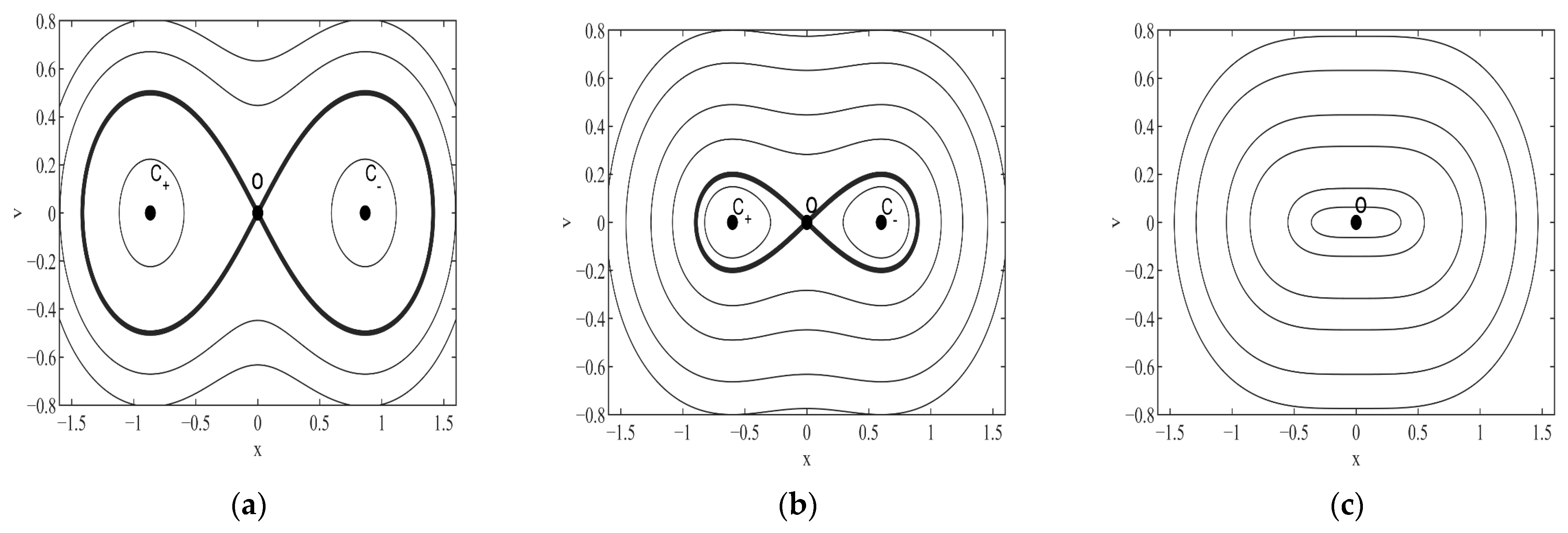
On this basis, the potential function and the phase portraits of the unperturbed system (5) for different values of the smoothness parameter
are depicted in
Figure 2 and
Figure 3, respectively. The thick curves in
Figure 3 show that there are symmetrically double potential wells in the system when
is 0.5 or 0.8. Comparatively, each potential well for
= 0.8 is much smaller than that for
= 0.5. In
Figure 3a,b, closed orbits near the non-trivial equilibria
are within the domains surrounded by homoclinic orbits, while closed orbits near the trivial equilibrium
are outside of these domains. At
α = 1, there is only one center
(see
Figure 3c). It follows that the unperturbed system (5) undergoes a subcritical pitchfork bifurcation at
= 1. Since bistability is common in the double-well case [
21,
22], using the parameters
we may observe the interaction among the coexisting attractors of the system (3) with the variation of the excitation parameters.
4. Attractors and Their Fractal Basins of Attraction
Apart from the variation in the excitation amplitude and frequency, the initial conditions can also lead to jumps among multiple attractors, thus having a significant effect on the dynamical behavior of the SD oscillator. This also suggests the necessity of classifying the basins of attraction (BA) of the attractors, namely the union of initial conditions triggering the same response [
1,
19]. The point mapping method [
24,
25] is utilized to depict the BA of the SD oscillatory system (3) on the initial-value plane
consisting of
array of points, which respects the initial conditions. For the same attractor, all initial conditions leading to it are marked in the same color. The sequences of the coexisting attractors and their BA with the variation in the excitation parameters are presented in
Figure 7 and
Figure 8. There are two columns in each figure: the left and right columns show the phase maps of the coexisting attractors and their BA, respectively. Here, the color to mark each attractor is the same as that of its BA.
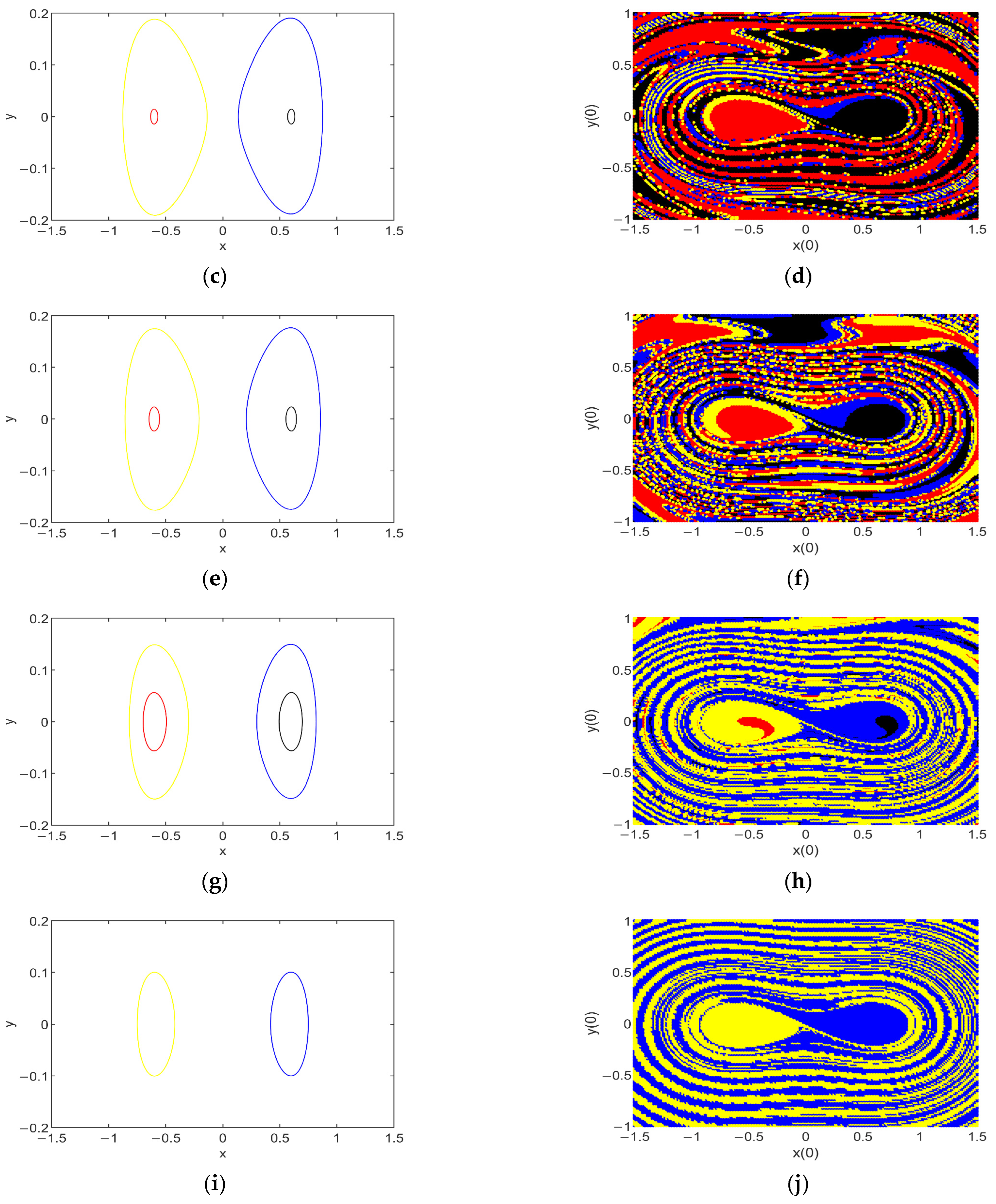
Given
, the evolution of the responses and their BA with an increase in the dimensionless excitation frequency
ω are shown in
Figure 7, where
varies within the range of [0.2, 0.6]. As shown in
Figure 7, there is no inter-well attractor, which is in agreement with the prediction of
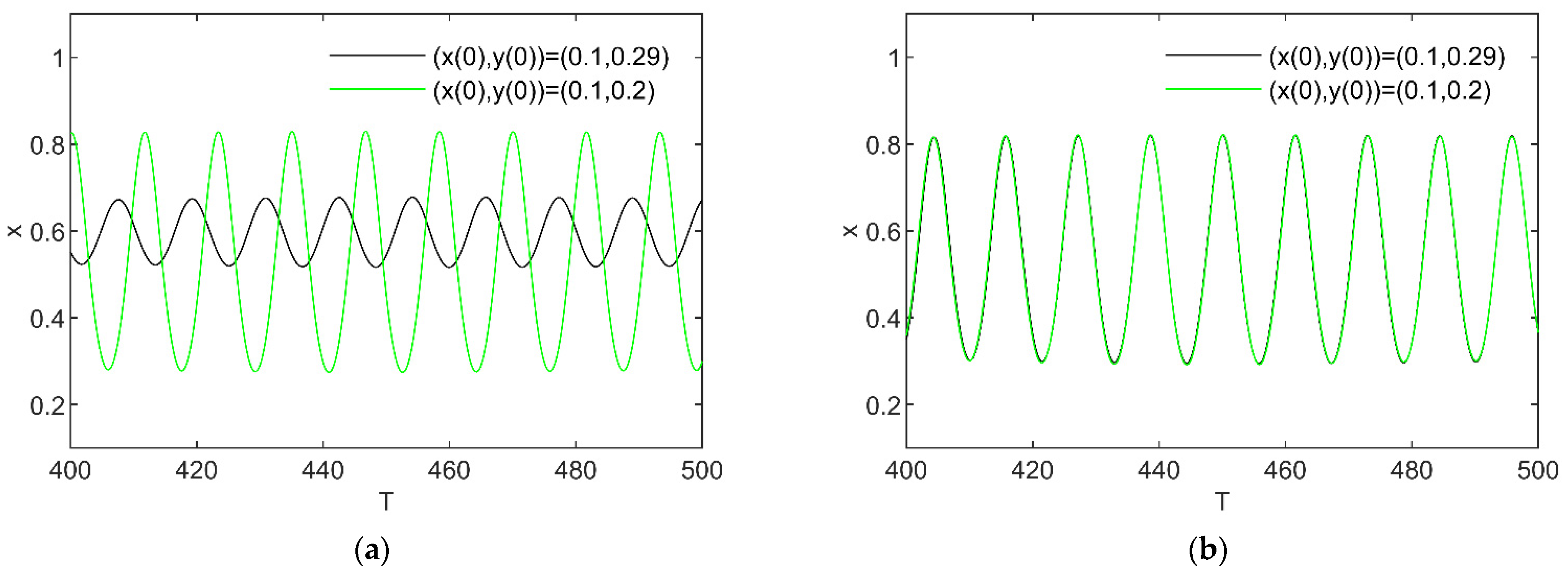
Figure 6a. For
, there are two intra-well attractors around the symmetric nontrivial equilibria
, which are marked in red and black, respectively (see
Figure 7a). The neighborhood of each nontrivial equilibrium is single-colored, meaning that the intra-well periodic attractors are locally stable. Comparatively, outside of the neighborhood of
, the BA of the attractors are intermingled, indicating a high probability of a jump between two attractors.
As the value of
is increased to 0.45 (see
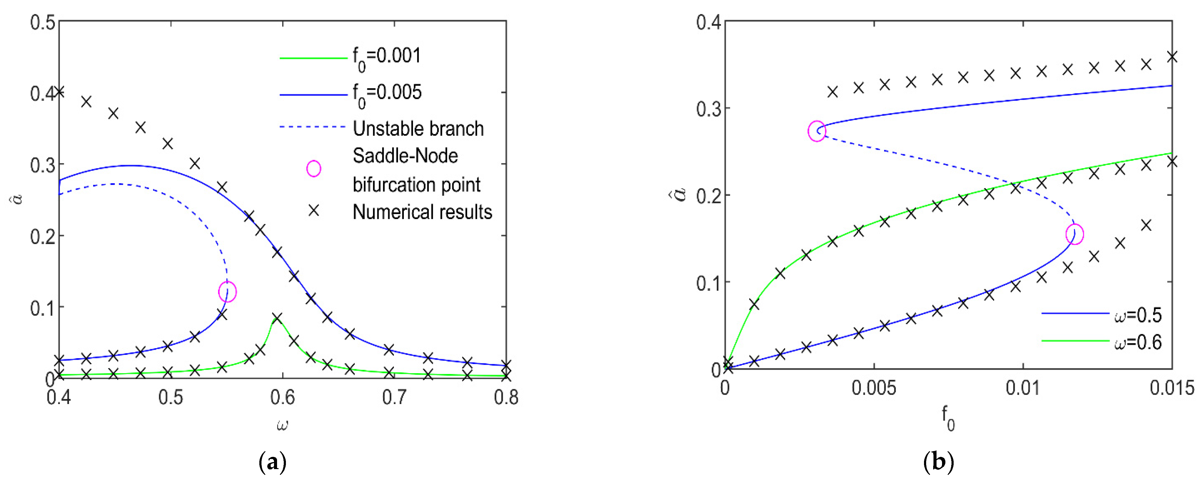
Figure 7c), these intra-well attractors still coexist, and their amplitudes are enlarged. Additionally, two new intra-well attractors with higher amplitudes appear, which can be ascribed to the saddle-node bifurcation depicted in
Figure 4a. As shown in
Figure 4d, even though the BA boundaries of the two lower-amplitude periodic attractors are fractal, these attractors are still locally stable. In contrast, the BA of the two higher-amplitude attractors, which are marked in yellow and blue, respectively, are too fractal and discrete to be detected, showing that their occurrence probability is pretty low. Thus, they are the so-called rare attractors [
26]. Since their BA are not in the vicinity of
, they can also be named as the hidden attractors [
27,
28].
As
is further increased (see
Figure 7e–h), the four intra-well attractors still coexist, but their amplitudes are changed: the amplitudes of the smaller intra-well ones become enlarged, while the amplitudes of the bigger ones become smaller. Meanwhile, the BA of the two smaller attractors are eroded by the BA of the bigger ones steadily, as depicted in
Figure 7f–h, illustrating an increase in the occurrence probability of the two bigger attractors. During this period, jumps among the four attractors can be triggered easily by a small change in the initial condition.
When the value of
reaches 0.60 (see
Figure 7i,j), the two lower-amplitude attractors vanish, and the higher-amplitude ones are no longer rare or hidden attractors.
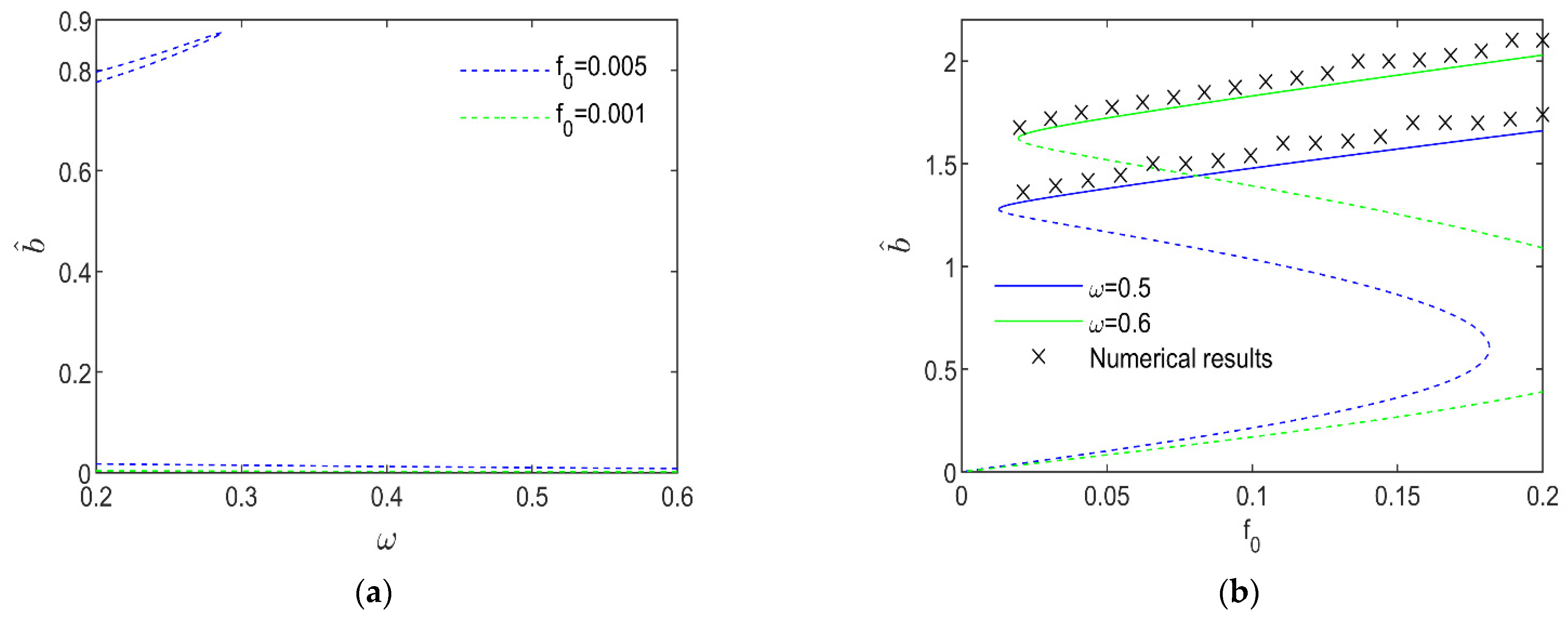
Figure 6 suggests that with an increase in
, the higher-amplitude intra-well attractors may replace the lower-amplitudes ones steadily, thus verifying the validity of the analytical results in the last section.
For
ω = 0.50, the sequences of the coexisting attractors and the extent of their BA with an increase in the dimensionless excitation amplitude
f0 can be observed in
Figure 8, which is more complicated than the evolution in
Figure 7.
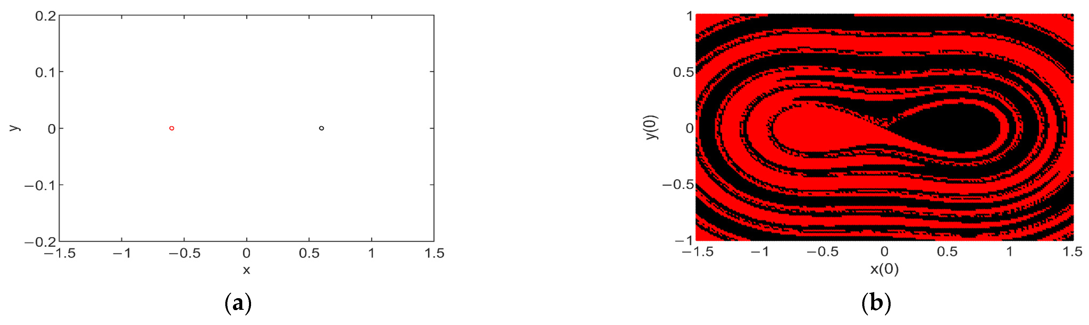
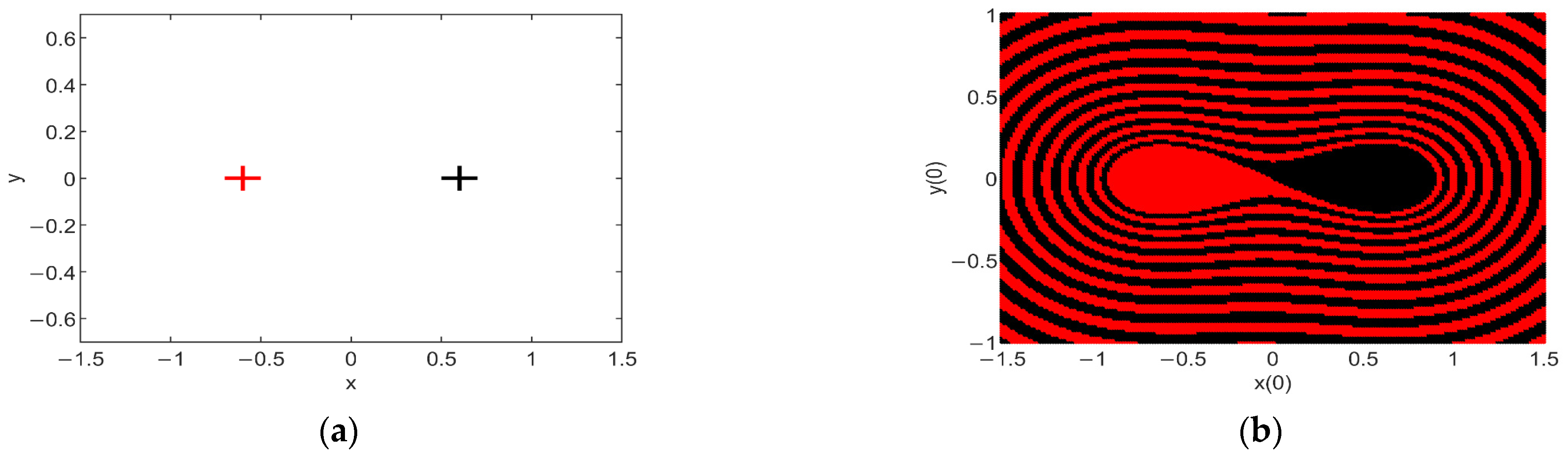
To begin with, for
, there is no excitation in the system (3) and the nontrivial equilibria
are stable (see
Figure 8a). The boundary separating their BA is smooth, as shown in
Figure 8b. An initial condition point chosen in the vicinity of
or
will surely lead to the corresponding nontrivial equilibrium. Comparatively, a small disturbance of the initial condition in the vicinity of
O(0,0) may lead to a jump from one equilibrium attractor to the other.
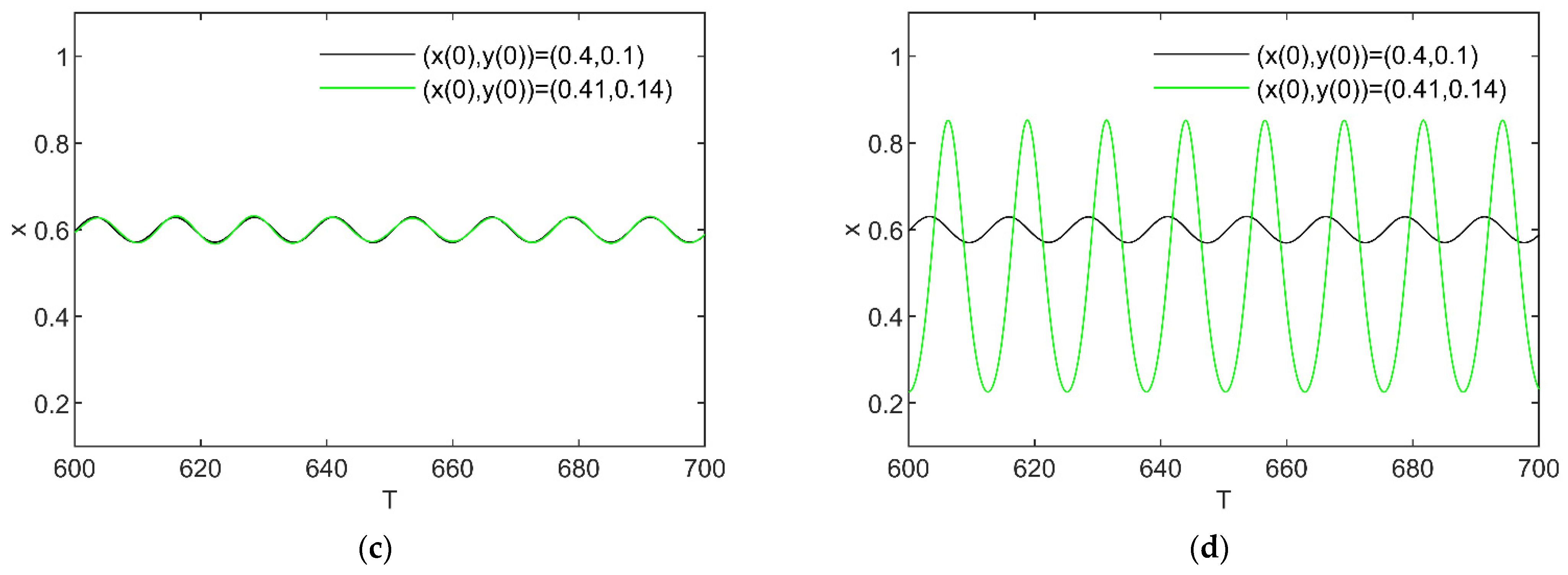
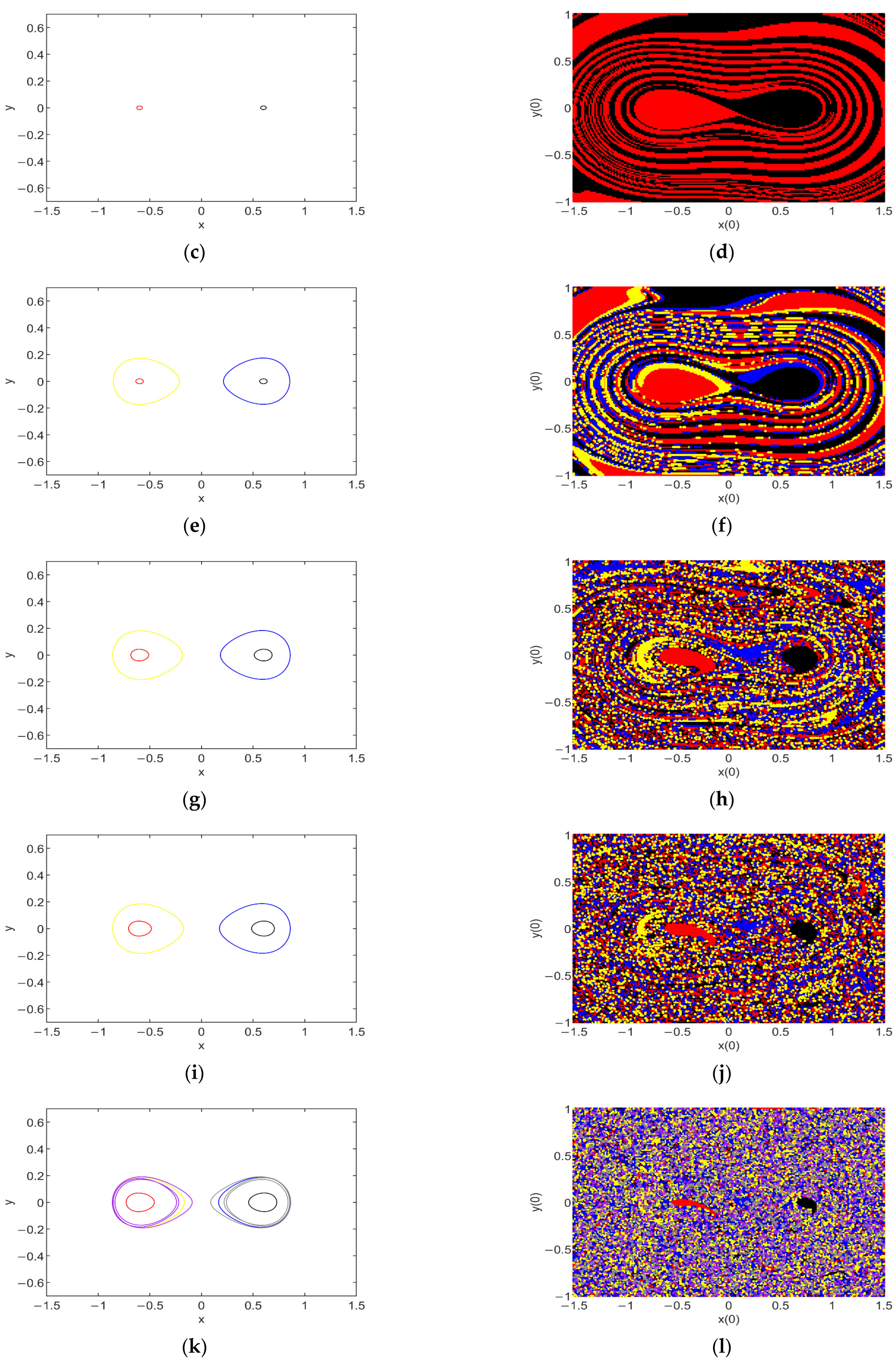
As
increases, the two nontrivial equilibria lose their stability; instead, there are two intra-well periodic attractors around the two equilibria. For instance, for
and
, the BA for the bistable attractors are similar, while those of the corresponding attractors are totally different (see
Figure 8a–d).
For
= 0.004, two new intra-well periodic attractors appear which amplitudes are higher than the former ones (see the yellow attractor and the blue one in
Figure 8e). It follows from
Figure 8f that the new attractors are rare and hidden attractors. As
further increases from 0.004 to 0.011 (see
Figure 8e–j), the BA of these four intra-well attractors are broken into discrete pieces and points.
For
, in addition to these four intra-well periodic attractors, two symmetric intra-well period-3 attractors surrounding
appear (see the purple and grey phases in
Figure 8k). Simultaneously, the BA of the six intra-well attractors are severely fractal (see
Figure 8l), demonstrating the high initial-condition sensitivity of the final behavior of the system (3).
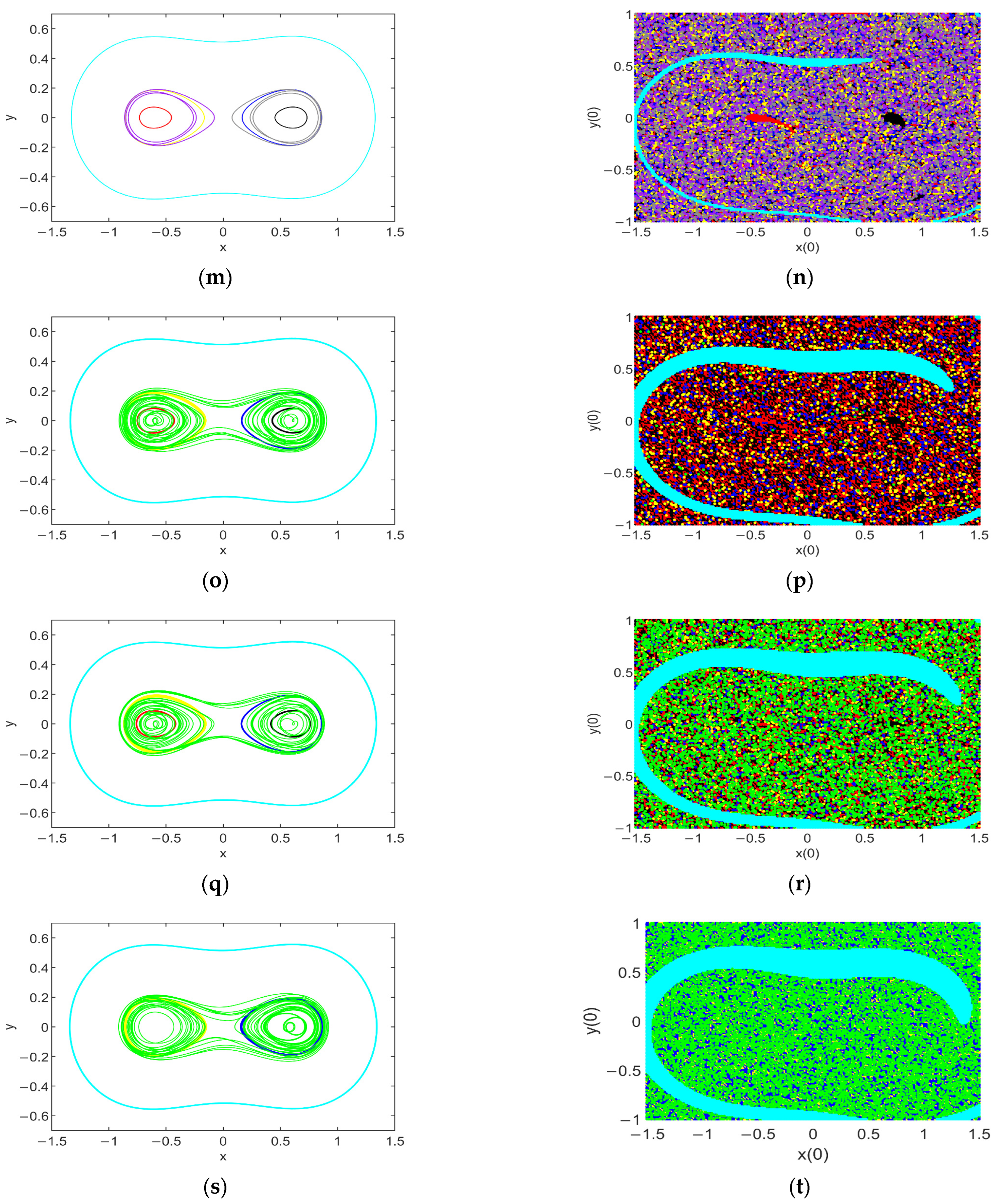
As
increases to 0.013, besides the six attractors, an inter-well periodic attractor near
O(0, 0) appears, as displayed in the light blue phase and the BA in
Figure 8m,n, respectively. This agrees perfectly with the prediction in
Figure 6b. Since its BA is small and beyond the vicinity of
O(0,0), it is also a rare and hidden attractor. It is worth mentioning that the BA of this inter-well attractor has a smooth boundary.
For
= 0.014 (see
Figure 8o), the period-3 attractors vanish; instead, an inter-well complex attractor traveling around the two nontrivial equilibria appears. Moreover, based on the nature of the BA in
Figure 8r, this attractor and the four intra-well attractors are all hidden attractors. As
further increases, the BA of the inter-well periodic attractor and the complicated one expands. Since the BA of the latter is discrete and mixed with the BA of the intra-well attractors, a jump among these attractors is easily incurred by a small disturbance of the initial condition. For
= 0.15, two intra-well attractors vanish (see
Figure 8s), which is in agreement with the prediction in
Section 3. In this case, only the BA of the inter-well periodic attractor is continuous with a smooth boundary, showing a higher occurring probability of this attractor.
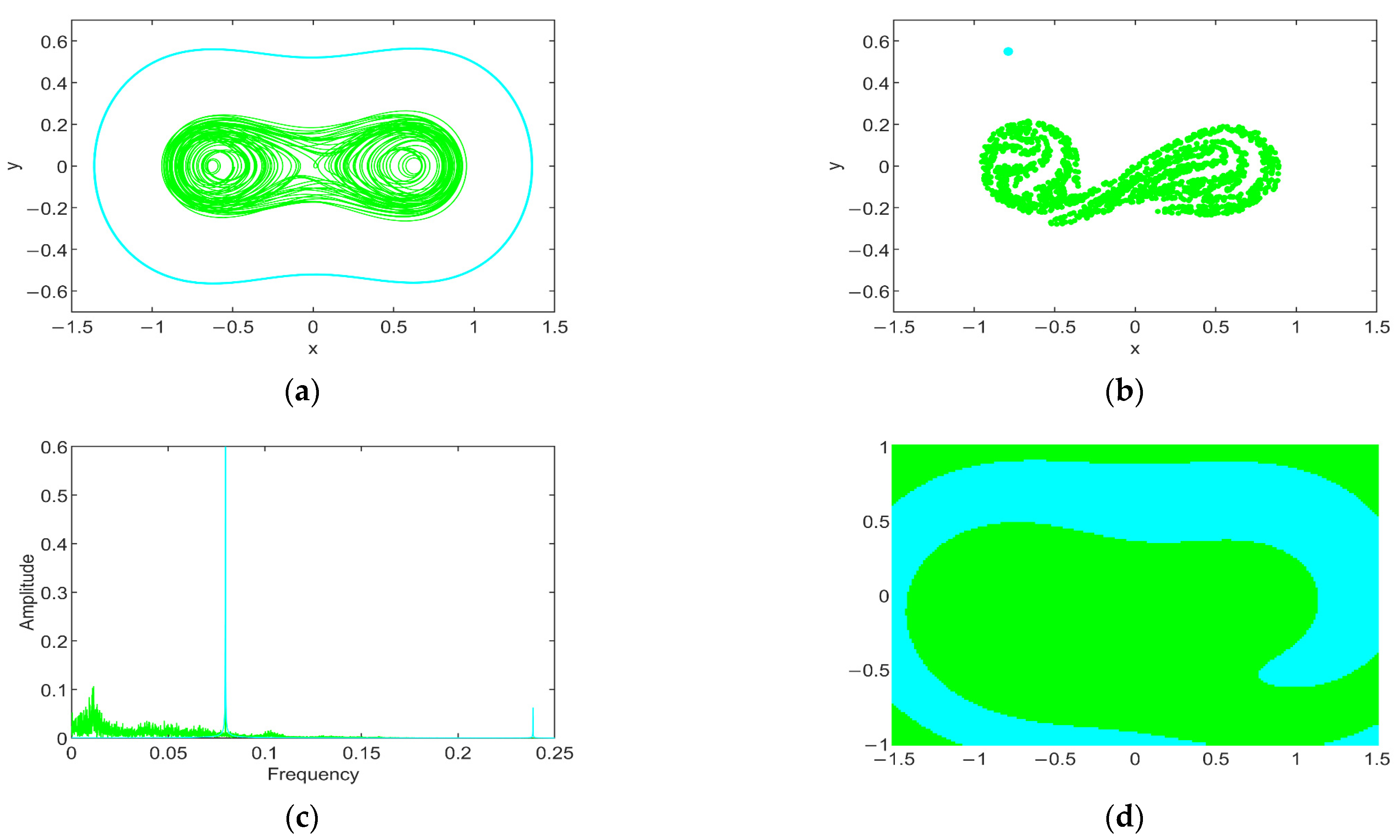
Finally, when
reaches 0.02, the intra-well attractors vanish, and only two inter-well attractors coexist in the system (3), i.e., a large-amplitude periodic attractor and a chaotic one, as depicted by the phase map, Poincare map, and frequency spectrum in
Figure 9a–c, respectively. Note that the boundary that separates the BA of the chaotic attractor and the large-amplitude periodic attractor is smooth (see
Figure 9d).
5. Conclusions and Discussion
In this paper, the multistability and the consequent jump of the harmonically excited SD oscillator were investigated. For the case wherein the nonlinearity of the oscillatory system is continuous, the intra-well periodic responses perturbed from the non-trivial equilibria and the inter-well responses near the trivial equilibrium were predicted, which results are in great agreement with the numerical results.
Given the value of the dimensionless smoothness parameter within the range (0, 1), there are double potential wells in the SD oscillatory system, thus exhibiting multistability. On this basis, we employed two analytical methods, namely, the method of multiple scales and the average method, to present the forms of the intra-well periodic solutions and the inter-well ones, respectively. It was found that, owing to the saddle-node bifurcation of the intra-well periodic solution, jumps between stable intra-well solution branches can be triggered by the excitation-frequency sweep or the increase in the excitation amplitude, leading to bistability in the vicinity of each non-trivial equilibrium. Moreover, the inter-well response can also be induced by increasing the excitation amplitude due to the saddle-node bifurcation of the inter-well solution.
The difference between the two theoretical methods is worth noting. When applying the method of multiple scales, it is not difficult to observe the decay between the analytical results of the intra-well responses and the numerical simulations under a higher excitation amplitude or a much lower excitation frequency. This can be ascribed to the limitation of this method, i.e., the prediction of this method can be quantitatively accurate if the excitation frequency is within a small vicinity of natural frequency and the excitation amplitude is low. Yet, this method is useful, considering its valid qualitative analysis and the convenience of presenting the analytical form of the periodic solutions through it. Comparatively, when utilizing the average method, we can predict more accurate periodic solutions. However, there are complete elliptic integrals in the form of inter-well periodic solutions, implying that the results are semi-analytical.
When increasing the excitation amplitude, we can also observe complex attractors, such as period-3 ones and chaotic ones, coexisting with the periodic attractors. According to the sequences of basins of attraction, with an increase in the excitation parameters, jumps among multiple attractors can be easily incurred by a tiny disturbance of the initial condition. An increase in the excitation frequency or amplitude may break the basins of attraction into discrete pieces and points, thus leading to hidden attractors.
Moreover, for a higher excitation amplitude, bistable inter-well attractors, namely, a chaotic attractor and a large-amplitude periodic attractor, can also be found in the SD oscillatory system. It is worth mentioning that the boundary separating their BA is not fractal but smooth.
Since jumps among multiple attractors could be catastrophic or desirable in practice, the results obtained in this study may provide potential values in the design and applications of oscillatory systems with strong geometric nonlinearities.


