Article

Cascade Control for Two-Axis Position Mechatronic Systems

Department of Automation, Technical University of Cluj-Napoca, Str. G. Bariţiu nr. 26-28, 400027 Cluj-Napoca, Romania
*
Author to whom correspondence should be addressed.
These authors contributed equally to this work.
Fractal Fract. 2023, 7(2), 122; https://doi.org/10.3390/fractalfract7020122
Submission received: 28 December 2022 / Revised: 23 January 2023 / Accepted: 25 January 2023 / Published: 28 January 2023
(This article belongs to the Special Issue Applications of Fractional-Order Calculus in Robotics)

Abstract

:
The current paper proposes an extension for two controller design procedures for a two-axis positioning mechatronic system, followed by a comparison between them. As such, the first method consists in formulating an optimization problem in terms of linear matrix inequalities (LMIs) in order to impose the location of the closed-loop poles, considering an uncertain model of such a system. The uncertain model is treated using various forms of linear differential inclusions (LDIs), namely, polytopic LDI (PLDI) and diagonal norm-bound LDI (DNLDI). Additionally, the problem regarding the command signal constraints is characterized in terms of LMIs. The imposed structure of the controller is a cascade one, with a PI controller for the position loop and a P controller for the velocity loop, having an additional feedforward term. On the other hand, the second method consists in designing a cascade controller with an inner P controller, as in the previous method, the outer controller being a fractional-order I λ I D λ D ( F O I D ) controller. In terms of degrees of freedom, both methods present four degrees of freedom for each axis. The presented controller design procedures will be applied for a numerical example of such a positioning system, and a comparison of the obtained performance metrics will be performed.

1. Introduction

1.1. Literature Review

Recent years have been marked by an increase in the popularity of position-based mechatronic systems, especially due to the technological level they have reached, in terms of speed, performance and versatility [1]. In order to have the resulting performance at the highest possible level, it is necessary for the control system to ensure a good reference tracking in a short time, without overshoot. Moreover, one of the main problems which a control system must deal with for such an equipment consists in parametric uncertainties. To take all these into consideration, rather than classical control techniques, other methods are proposed in recent studies, based on robust, fractional or adaptive control approaches.
Starting from the classical control methods based on the idea of pole placement, the authors of [2] present the principle according to which, to ensure a certain transient response, it is not necessary to place the poles in an exact location, but in a certain region in the complex plane. These regions are called D -regions, being convex and symmetrical to the real axis. Thus, by solving a set of linear matrix inequalities (LMIs), the state feedback matrix which ensures D -stability (i.e., all poles of the resulting closed-loop system are placed into a certain D -region) is obtained. The possibility to include and overimpose many design requirements, like transient response performances, command signal saturation constraints and model uncertainties, illustrates the great advantage of LMIs [3].
Due to its powerful advantage, the LMI-based control approach was proposed for various processes and applications. In [4], the authors proposed an LMI approach to design a H fuzzy controller with pole location constraints. Moreover, Ref. [5] presents an LMI-based control design that deals with the stabilization of a bilinear system with a guaranteed stability region. Parametric uncertainties are included in the control design problem using LMIs for a wind turbine, in [6], proving that using this approach better performances are obtained compared with those obtained using a classical designed controller. The journal paper [7] proposes an LMI-based H output-feedback controller, taking into consideration the input and output delays from sensors and actuators for a vehicle roll stability problem. In the conference paper [8] regarding LMI-based controllers, the authors present an energy-based control strategy with nonlinear state feedback controller for a quadrotor used for transporting payload.
In the case of PWM-driven voltage converters, an LMI-based approach used for robust linear-quadratic-regulator (LQR) design is presented in the paper [9], alongside the work of [10] in which a similar approach is considered for robust structured controller design. An LMI use case is also compared to a linear-quadratic-Gaussian (LQR) control in the paper [11], which proved that the proposed approach presented clear improvements for a MIMO helicopter process modelled at variable operating points. In the case of a pressure control process on wet clutches, as studied in the work [12], favorable results have been obtained regarding both robustness to sensor noise and modeling errors, alongside performance indices in the transient response of the closed-loop system.
Fractional-order PID controllers generalize classical PID controllers by adding extra degrees of freedom which proved to be more robust for many benchmark problems. In [13], the authors proposed a fractional-order PID (FO-PID) controller designed in order to meet both robustness and performance specifications for a DC motor used in a mechatronic system. Better performance indices have also been found in DC motor control with uncertainties and nonlinear dynamics using FO-PI regulators in [14]. Improved performances by also obtaining a reduced-order regulator through intelligent H techniques have been reported in [15], while a general-purpose quasi-experimental method which generalizes the well-established Kessler’s symmetrical optimum principle was proposed and implemented in [16]. Moreover, a simple tuning method based in the limit cycle oscillations is proposed in [17], with application on a DC servo motor. Such a FO-PID regulator for a two-axis CNC machine is proposed in [18], designed using μ -synthesis and the minimization problem is solved using a metaheuristic Artificial Bee Colony (ABC) algorithm. In a similar manner, a different application for a highly-nonlinear twin rotor aerodynamic system with its inherent difficulties, has been studied in [19]. The integration of the fractional-order design into the robust control framework gathers the advantages of both control domains, as presented in [20]. Extensions of FO regulators directly designed for fractional-order plants have been proposed in [21,22], where the first paper presents a comprehensive theorem and corresponding algorithm for the robust stabilization problem, while the latter proposes and discusses a novel graphical tuning method for such control systems.
Position-based mechatronic systems are widely used in industry and mainly in production lines and manufacturing. Because of this, it is necessary for the control system to ensure high precision and response speed. In the last years, many studies have been made in order to find the best option when it comes to the design procedures and controller types for these classes of positioning systems. Although classical controllers are mainly used [23], such as P, PI or PID controllers, in cascade configuration or not, more advanced design techniques are proposed. In [24], an optimal ABC-based LQR is proposed, and in another paper [25], we propose a cascade control configuration obtained based on the state feedback gains designed by solving LMIs.

1.2. Contributions

The current paper proposes two control structures for an uncertain two-axis mechatronic positional system: one using the state-feedback approach, by extending our previous paper’s results [25], and one based on the behavior of bringing the system to a limit cycle, which extends the ideas presented in [17]. Based on the literature review performed in the previous subsection and their limitations, the main contributions of the current paper are:
(i)
To include the parametric uncertainties of a two-axis mechatronic positional system into the LMI-based control problem in order to impose a D -region where the poles are real and under a prescribed value, by converting the linear differential inclusion (LDI) into a polytopic LDI (PLDI), against the initial method proposed in [25], where the problem has been formulated for the nominal model of a single axis positional system;
(ii)
To reduce the size of the resulting LMI-based control problem by converting the PLDI into a diagonal norm-bound LDI (DNLDI), and to include the constraints given by the saturation phenomenon which appears on the command signal, which has not been considered in the previous paper even for the case of nominal system;
(iii)
To impose a specific structure on the LMI variables such that the resulting state-feedback can be converted into a cascade control structure for both axes, using a similar idea as in [25] for a single axis;
(iv)
To present an autotuning-type design procedure for a fractional-order integral-derivative controller by considering a relay-type nonlinearity to force a limit cycle to obtain the value of the gain-crossover frequency, and then to impose the desired phase margin, by extending the idea from [17];
(v)
To perform a set of numerical simulations to compare the performance obtained with the proposed methods in terms of quantifiable metrics, such as settling time, rise time and overshoot, robustness and implementability.

1.3. Paper Structure

The rest of the paper is organized as follows. Described in Section 2 is the LMI-based problem formulation to impose the D -stability through a full state-feedback. Section 3 presents the two-axis positional mechatronic system, along with the possibility to convert the full state-feedback controller into a cascade control structure. The second controller design procedure is described in Section 4, while Section 5 presents the obtained results. A thorough discussion and a set of further research directions are given in Section 6, and the paper closes with some conclusions in Section 7.

2. State Feedback Controller

The purpose of the current section is to briefly describe the LMI approach to design a state feedback controller for a system described using a polytopic linear differential inclusion (PLDI). To impose a performance set, the D regions will be used. Consider a continuous-time PLDI described by:
Σ δ : x ˙ ( t ) = A ( δ ) x ( t ) + B ( δ ) u ( t ) ,
where x R n x , u R n u , δ U δ R n δ is the uncertainty from the state and input matrices, and U δ closed and bounded. The PLDI should be characterized by the following L-vertex convex hull:
( A ( δ ) , B ( δ ) ) | δ U δ Ω Conv ( A i , B i ) , i = 1 , L ¯ .
Assumption 1. 
Each pair ( A ( δ ) , B ( δ ) ) with δ U δ is detectable.
Considering a full state feedback matrix K R n u × n x which gives the control law u = K x , the following PLDI closed-loop system results:
x ˙ ( t ) = A ( δ ) + B ( δ ) K A o ( δ ) x ( t ) .
To ensure the asymptotic stability of the closed-loop autonomous system from (3), a quadratic Lyapunov function V : R n x R + having the structure V ( x ) = x P x should be constructed. To construct such a quadratic function, the following linear matrix inequalities should have a common solution P S n x + :
A o ( δ ) P + P A o ( δ ) < 0 , δ U δ ,
which is an uncountable set of LMIs. However, using the convex hull Ω from (2), the feasibility problem which guarantees the asymptotic stability of the closed-loop system is:
P S n x + and ( A i + B i K ) P + P ( A i + B i K ) < 0 , i = 1 , L ¯ .
However, the problem is to design a state feedback, so the set of LMIs from (4) are bilinear matrix inequalities (BMIs), which are not convex by nature. However, using the substitution Z = K P R n u × n x , the resulting problem can be described using LMIs:
Find P S n x + and Z R n u × n x such that A i P + P A i + B i Z + Z B i < 0 , i = 1 , L ¯ .
A feasible point from the convex cone of the solution of the problem (5) leads to a stabilizable feedback K = Z P 1 for the PLDI. If an additional set of requirements should be imposed, the closed-loop eigenvalues must be placed into a specific region of the complex plane. Each convex region symmetrical to the real axis can be expressed using a combination of transformations given by two matrices L , M R m × m , L = L :
D ( L , M ) = λ C : L + λ M + λ * M < 0 .
Definition 1 
([26]). A matrix A R n x × n x is D -stable if all its eigenvalues lie in a convex region D ( L , M ) defined in (6). This D -stability is characterized using the LMI approach as follows:
M D ( A , P ) = L P + M ( A P ) + M ( P A ) < 0 ,
where ⊗ is the symbol for the Kronecker product.
For the purpose of this paper we consider only two regions: the vertical strip and the conic sector. The vertical strip is used to impose the condition of having real part less than a prescribed value α < 0 , which imposes one important closed-loop performance regarding the settling time: t s 4 | α | . On the other hand, the conic sector is used to impose:
λ + λ ¯ | λ λ ¯ | π tan θ ,
which leads to having a damping factor ζ cos ( θ ) , thus, implying a limitation for the overshoot of the closed-loop system. For the vertical strip the D -region is characterized using L = 2 α and M = 1 , while for the conic region L = 0 and M = R θ are used, where R θ is the 2 × 2 matrix corresponding to the rotation with angle θ . We further call this region as a D ( α , θ ) -region. A set of necessary and sufficient conditions to ensure D ( α , θ ) -regional stability for a PLDI system ( Σ δ ) is presented in the following theorem.
Theorem 1 
( D -stability controller [3]). All eigenvalues of the closed-loop system A c l ( δ ) A ( δ ) + B ( δ ) K could be set in a specific D ( α , θ ) -region if and only if all pairs ( A ( δ ) , B ( δ ) ) , δ U δ , are controllable and there are two matrices P S n x + and Z R n u × n x such that:
A i P + B i Z + ( A i P + B i Z ) 2 α P < 0 , i = 1 , L ¯ ,
A i P + B i Z + ( A i P + B i Z ) 1 tan θ ( A i P + B i Z ( A i P + B i Z ) ) 1 tan θ ( A i P + B i Z ( A i P + B i Z ) ) A i P + B i Z + ( A i P + B i Z ) < 0 , i = 1 , L ¯ .
Then the full state feedback gain is given by K = Z P 1 .

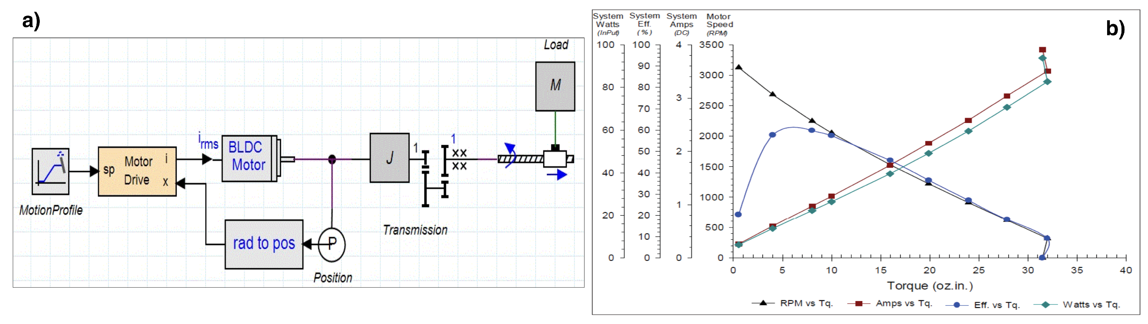
3. Position-Based Mechatronic System

3.1. Plant Model

The described plant is a general purpose two-axis positional system, each axis being operated individually by a servo motor. In this paper, a translational two-axis Computer Numerical Control machine (CNC), also used in our previous works [25,27], will be considered. The mathematical model of the system can be written as follows:
G δ ( s ) : ω ˙ x ( t ) θ ˙ x ( t ) ω ˙ y ( t ) θ ˙ y ( t ) θ x ( t ) θ y ( t ) = 1 T M x 0 0 0 K M x T M x K x y 1 0 0 0 0 0 0 0 1 T M y 0 K y x K M y T M y 0 0 1 0 0 0 0 1 0 0 0 0 0 0 0 1 0 0 ω x ( t ) θ x ( t ) ω y ( t ) θ y ( t ) u x ( t ) u y ( t ) ,
where ω x , ω y , θ x and θ y are the angular speeds and the positions of the X axis and Y axis, respectively, while u x , u y 1 , 1 are the duty cycles, scaled to relative values, of the PWM command signals for each axis. The mathematical model has been obtained based on a priori knowledge of the physical process and then fine-tuned using system identification techniques. The electrical part presents a time constant which can be neglected against the time constant of the mechanical part, resulting in a first order model for the system from input command to angular speed. Moreover, the mechanical part presents a set of nonlinearities mainly as a result of Coulombian friction, leading to slightly different values of the model’s parameters. As such, these parameters present uncertainties which encompass differences appearing in various equilibrium points. Such differences lead to the system G δ , possible to be described using a PLDI.
The first method proposed in this paper implies an extension of finding a cascade structure from [25], comprised of a P I controller for the outer position loop and a P-type controller for the inner velocity loop. In our previous work, the controller gains have been computed using an optimal full state feedback gain matrix which is a solution for the nominal case of the LMI problem described in Section 2. The main improvement of this particular method considered in this paper consists in finding the optimal state-feedback which satisfies the constraints imposed through regional LMIs for both the nominal and uncertain plants, as in Theorem 1. As such, the initial plant model must be augmented with two additional states z x and z y having the state equations z ˙ x = θ x and z ˙ y = θ y . This augmentation leads to an extended uncertain state-space model:
G ¯ δ ( s ) : ω ˙ x ( t ) θ ˙ x ( t ) z ˙ x ( t ) ω ˙ y ( t ) θ ˙ y ( t ) z ˙ y ( t ) θ x ( t ) θ y ( t ) = 1 T M x 0 0 0 0 0 K M x T M x K x y 1 0 0 0 0 0 0 0 0 1 0 0 0 0 0 0 0 0 0 1 T M y 0 0 K y x K M y T M y 0 0 0 1 0 0 0 0 0 0 0 0 1 0 0 0 0 1 0 0 0 0 0 0 0 0 0 0 1 0 0 0 ω x ( t ) θ x ( t ) z x ( t ) ω y ( t ) θ y ( t ) z y ( t ) u x ( t ) u y ( t ) .
To model an uncertain parameter c [ c ̲ , c ¯ ] , the following transformation can be used:
c = c ( n ) + r c δ c , with r c = c ¯ c ̲ ,
where c ( n ) is the nominal value of the parameter and | δ c | 1 is a normalized uncertainty element. Using this transformation, the extended PLDI system can be converted into a diagonal norm-bound LDI (DNLDI) system, having the following state-space representation:
x ˙ ( t ) y ( t ) v ( t ) = A w i d t h B u w i d t h B d C y w i d t h D y u w i d t h D y d C v w i d t h D v u w i d t h D v d x ( t ) u ( t ) d ( t )
where x = ω x θ x z x ω y θ y z y R n x is the state vector, u = u x u y R 2 is the command input vector, d = d T M x d T M y d K M x d K M y d K x y d K y x R 6 is the disturbance input vector, y = θ x θ y R 2 is the output vector, and v = v T M x v T M y v K M x v K M y v K x y v K y x R 6 is the disturbance output vector. The matrices involved in the state-space realization are:
A = 1 T M x ( n ) 0 0 0 0 0 1 0 0 0 0 0 0 1 0 0 0 0 0 0 0 1 T M y ( n ) 0 0 0 0 0 1 0 0 0 0 0 0 1 0 B u = K M x ( n ) T M x ( n ) K x y ( n ) 0 0 0 0 K y x ( n ) K M y ( n ) T M y ( n ) 0 0 0 0 B d = 1 T M x ( n ) 0 1 T M x ( n ) 0 1 T M x ( n ) 0 0 0 0 0 0 0 0 0 0 0 0 0 0 1 T M y ( n ) 0 1 T M y ( n ) 0 1 T M y ( n ) 0 0 0 0 0 0 0 0 0 0 0 0
C v = 0 0 0 0 0 0 0 0 0 0 0 0 0 0 0 0 0 0 0 0 0 0 0 0 r T M x T M x ( n ) 0 0 0 0 0 0 0 0 r T M y T M y ( n ) 0 0 D v u = r K M x 0 0 r K M y r K x y 0 0 r K y x r T M x K M x ( n ) T M x ( n ) r T M x K x y ( n ) r T M y K y x ( n ) r T M y K M y ( n ) T M y ( n ) D v d = 0 0 0 0 0 0 0 0 0 0 0 0 0 0 0 0 0 0 0 0 0 0 0 0 r T M x T M x ( n ) 0 r T M x T M x ( n ) 0 r T M x T M x ( n ) 0 0 r T M y T M y ( n ) 0 r T M y T M y ( n ) 0 r T M y T M y ( n )
C y = 0 1 0 0 0 0 0 0 0 0 1 0 D y u = 0 0 0 0 D y d = 0 0 0 0 0 0 0 0 0 0 0 0 .
The conversion of a PLDI into DNLDI offers the possibility to avoid using L LMIs to impose the vertical strip region, leading to the following LMI problem: find P S n x + , T S n d + , and Z R n u × n x such that:
A P + P A + B u Z + Z B u 2 α P T B d + C v P + D y u Z T D v d + D v d T 2 T < 0 .
Additionally, to impose the allowed maximum command input in a symmetrical manner u [ u ̲ = u ¯ , u ¯ ] for an initial value of the state vector lying in the ellipsoid:
E Q = { x R n x | x Q x 1 } ,
with Q S n x + , the following LMI can be used:
diag ( u ¯ ) 2 Z Z Q 0 ,
where diag ( u ¯ ) is the diagonal matrix formed using the vector u ¯ .

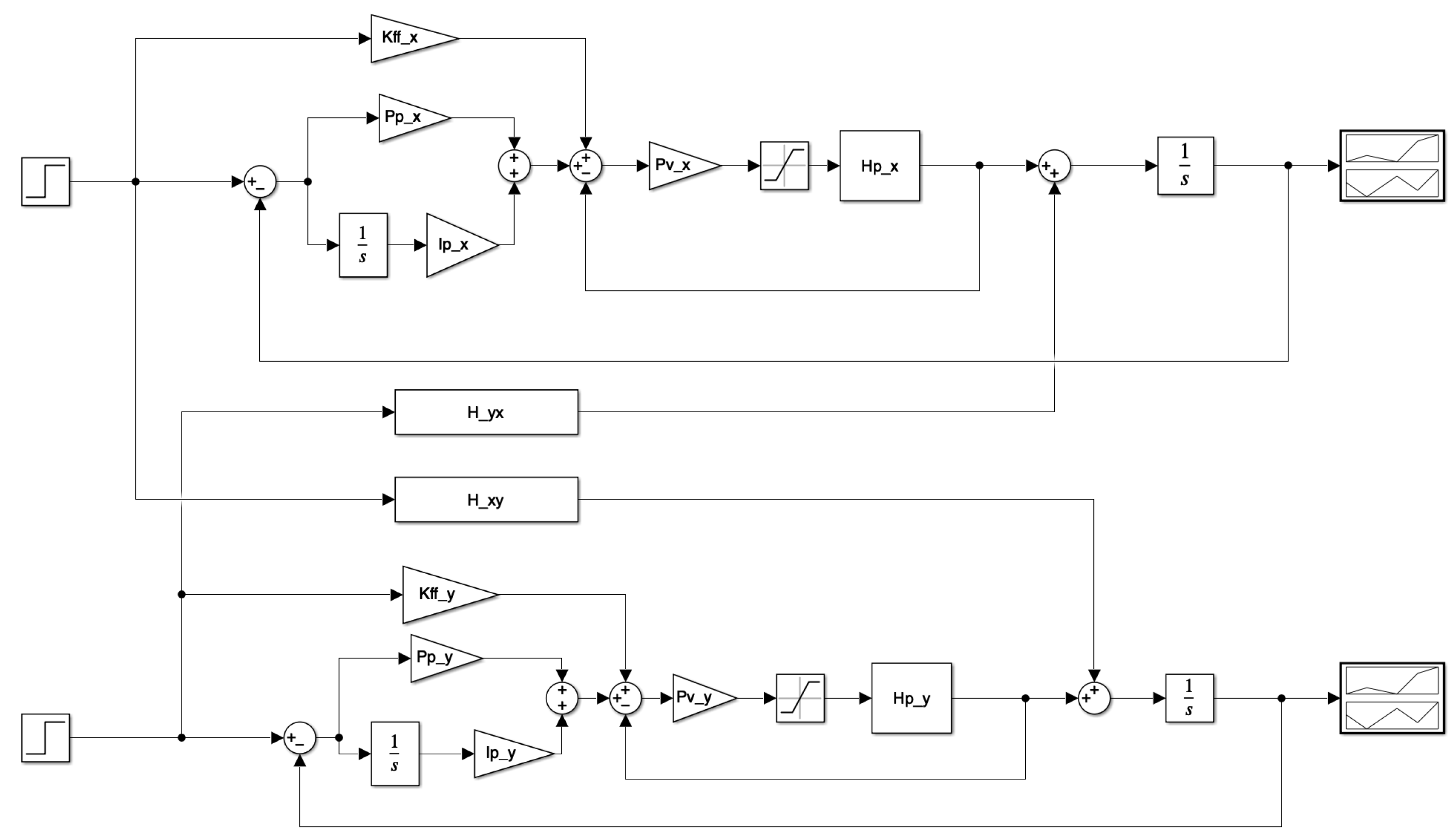
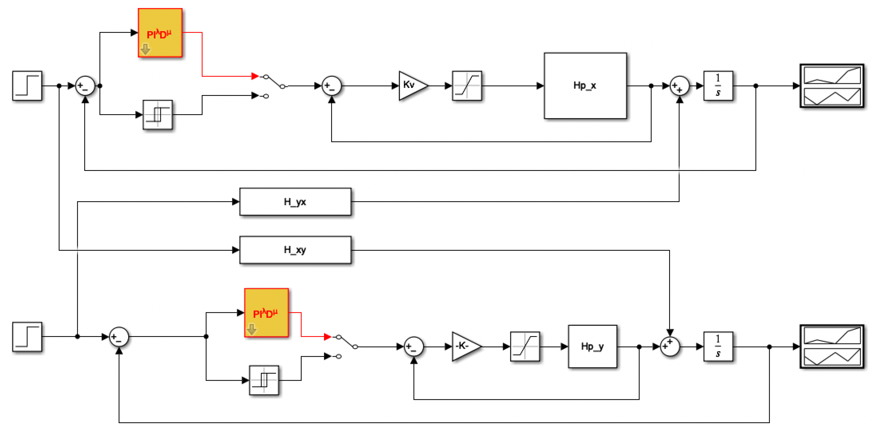
3.2. From State Feedback to Cascade Control

To convert the state-feedback control structure to a cascade control structure in the case of a two-axis mechatronic system, the following forms of the matrices P and Z will be considered:
P = P 1 O O P 2 S 6 + and Z = Z 1 O O Z 2 R 2 × 6 ,
with P 1 , P 2 S 3 + and Z 1 , Z 2 R 1 × 3 . The resulting form of the static state-feedback gain matrix K is:
K = k 1 k 2 k 3 0 0 0 0 0 0 k 4 k 5 k 6 .
For brevity, we consider the behavior on a single axis K 1 = k 1 k 2 k 3 0 0 0 , and we analyze the equivalence between the the control law given by the state-feedback and the control law given by the cascade structure. As such, on X-axis we have the following command signal given by the state-feedback approach:
u x , K ( t ) = θ x ( t ) + K 1 x ( t ) = θ x ( t ) + k 1 ω x ( t ) + k 2 θ x ( t ) + k 3 θ x ( t ) d t ,
with θ being the outer position loop reference signal. On the other hand, for a cascade control scheme having a P controller on the inner loop, along with a PI controller on the outer loop, the control law resulted in this case can be rearranged as:
u x , P I P ( t ) = P v ( x ) ω x ( t ) P p ( x ) θ x ( t ) I p ( x ) θ x ( t ) d t + P p θ x ( t ) + I p ( x ) θ x ( t ) d t ,
with inner loop proportional gain P v , and the pair P p and I p as the outer loop proportional and integral regulator gains, respectively. In the exact same manner, the signals u y , K and u y , P I P can be expressed. Therefore, using the relations exposed in Equations (19) and (20), the following equivalence between the aforementioned gains from the cascade control structure and those obtained using the state feedback controller can be performed:
P v ( x ) = k 1 , P p ( x ) = k 2 k 1 , I p ( x ) = k 3 k 1 ,
P v ( y ) = k 4 , P p ( y ) = k 5 k 4 , I p ( y ) = k 6 k 4 .

3.3. Feedforward Component

As noticed in Equations (19) and (20), an extra integral term in θ x appears in the cascade control structure case. As such, an extra analysis should be performed to emphasize this difference. For state-feedback control, the obtained transfer function from θ x to θ x is:
H o , K ( s ) = C y , 1 s I n A + B u , 1 K 1 1 B u , 1 = K M x T M x s ( s λ i ) ,
where λ i are the closed-loop state matrix A + B u , 1 K 1 eigenvalues, while the index 1 is used to mark the first row or column of the matrices which describes the augmented plant. Similarly, in the case of using the PI–P cascade control strategy, the resulting closed-loop transfer function from θ x to θ x becomes:
H o , P I P ( s ) = P v ( x ) K M x ( P p ( x ) s + I p ( x ) ) ( s λ i ) .
Therefore, in both cases, transmission zeros appear in closed-loop, causing changes in terms of the performance indices initially imposed through the position of the closed-loop system’s poles. For the state-feedback strategy for the augmented model, a transmission zero in the origin s ˚ = 0 is obtained. On the other hand, the cascade controller brings a transmission zero in the value s ˚ = I p ( x ) P p ( x ) .
To cancel the effect of the resulting transmission zero, the feedforward gain will be used as an additional degree of freedom. To cancel the closed-loop zero for the cascade control structure, the feedforward gains must be:
K f f ( x ) = P p ( x ) and K f f ( y ) = P p ( y ) .
Moreover, using this feedforward term, the integral action present on the reference manages to cancel the transmission zero s ˚ = 0 which shows in the state-feedback case. Therefore, the additional feedforward gains K f f ( x ) and K f f ( y ) lead to obtaining two closed-loop systems without transmission zeros, so the performances imposed through D -region are kept unchanged.

4. 4DOF Fractional-Order Controller

The previous section described a 4DOF controller for each axis organized in a cascade-type structure, having an outer loop PI controller and an inner loop P controller, along with a feedforward gain. It must be pointed out that this structure is imposed by the physical stand, as mentioned in [25]. In the current section we propose an alternative control structure having four degrees-of-freedom as well. As such, for each axis:
  • For the inner loop, a simple P controller is used;
  • For the outer loop, a particular structure of fractional-order PID controller is proposed:
    K F O I D ( s ) = K i · T i s + 1 s λ .
The differential equations which describe the dynamics of the velocities ω x and ω y in terms of command inputs u x and u y are:
ω ˙ x = 1 T M x ω x + K M x T M x u x + K x y u y ;
ω ˙ y = 1 T M y ω x + K y x u x + K M y T M y u y .
The inner P controllers K ω x and K ω y should be designed to impose the desired speed profile. The dynamics of the resulting inner closed-loop systems are given by:
H i n , X ( s ) = K ω x s + 1 T M x 1 + K ω x K M x and H i n , Y ( s ) = K ω y s + 1 T M y 1 + K ω y K M y .
For designing the F O I D controller we impose a limit cycle oscillation. Let us consider a symmetrical bipositional relay having a hysteresis width of ε and an amplitude h, denoted by R ( ε , h ) , having the inverse describing function:
N i ( R ( ε , h ) ) = π ε 4 h A ε 2 1 + j , A > ε ,
where A is the amplitude of the input sinusoidal signal. If such a nonlinearity is inserted into a negative feedback system next to a linear system, a stable limit cycle appears. The parameters of the resulting limit cycle can be determined using the intersection between the negative inverse description locus and the Nyquist diagram of the linear system. The limit cycle is characterized by a frequency ω osc and an amplitude A osc . Moreover, using the Fourier decomposition of N i R ( ε , h ) , the equivalent gain of the relay nonlinearity is:
K e q = 4 h π A osc .
The outer open-loop systems have the following dynamics:
H o l , o u t , i ( s ) = K ω i s s + 1 T M i 1 + K ω i K M i , i { X , Y } .
The time constant of the F O I D controller is set to be in both cases:
T 1 ( x ) = T M x 1 + K ω x K M x and T 1 ( y ) = T M y 1 + K ω y K M y ,
and we want to impose in each case the frequency ω osc of the resulting limit cycle as the gain-crossover frequency ω g c , while the fractional order of the integral effect is designed such that a prescribed value of the phase margin γ k is met. The resulting equation is:
γ k = arg ( N i ( R ( ε , h ) ) ) + arctan T 1 ( i ) ω osc λ ( i ) π 2 ,
which implies:
λ ( i ) = 2 π arg ( N i ( R ( ε , h ) ) ) + arctan T 1 ( i ) ω osc γ k .
Additionally, to ensure ω g c = ω osc , the gain of the F O I D controller should be:
K i = 4 h π A o s c ω osc λ 1 + T 1 ω osc 2 = K e q · ω osc λ 1 + T 1 ω osc 2 .

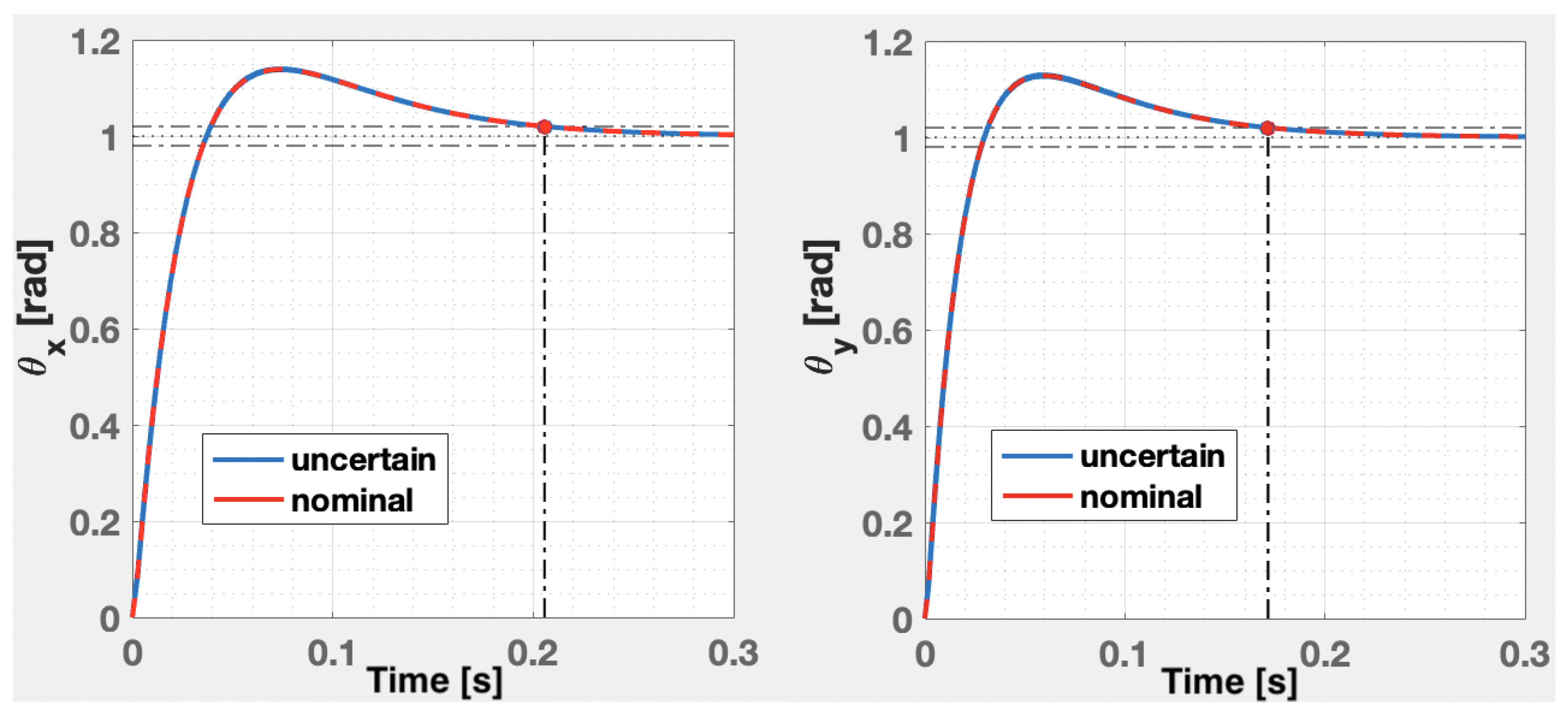
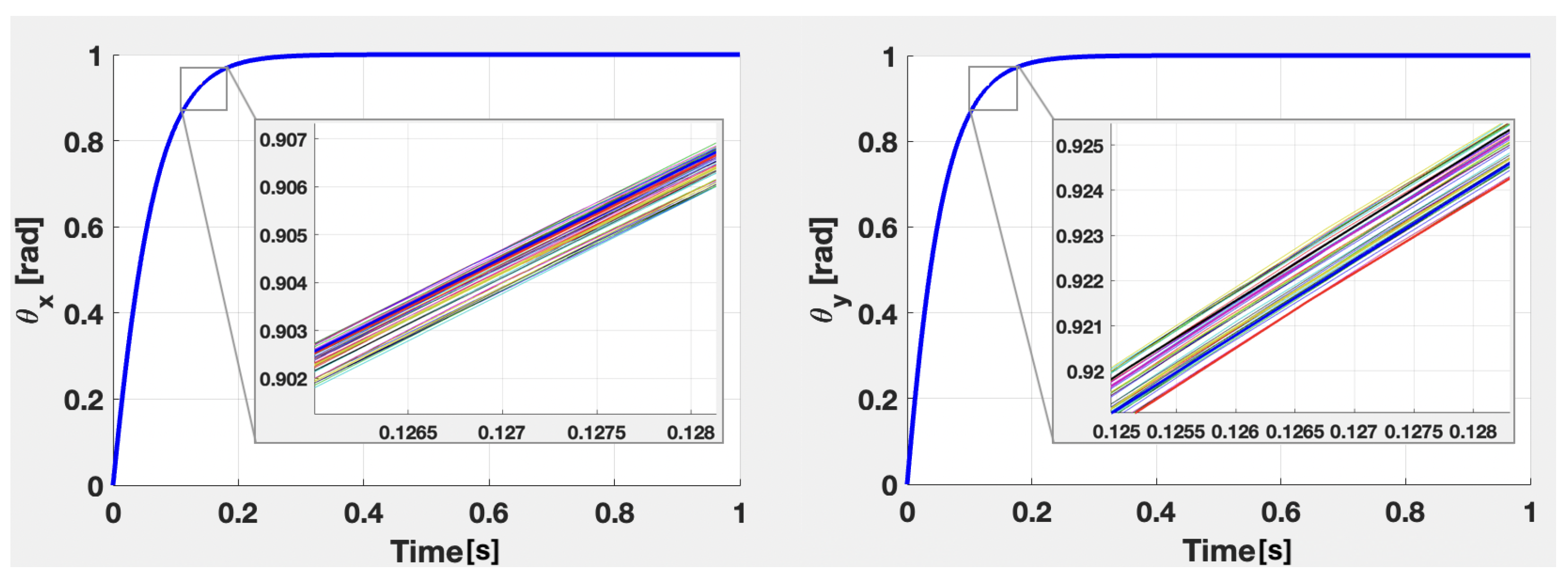
5. Numerical Results

The purpose of this section is to illustrate the numerical results obtained by implementing the proposed controllers for the plant described in Section 3.1. The mathematical model for the MIMO system was obtained based on the measured data in various operating points for the described two axes of the mechatronic system. The mechanical system inherent to each CNC axis is presented in Figure 1a), showing its components and interconnections, alongside the brushless DC (BLDC) motor characteristics involved in the system dynamics in Figure 1b). The actuation, measurements and control laws are managed through a Siemens CNC Sinumerik and MC206X Motion Coordinator devices. As such, considering various persistent inputs around a value u 0 , i.e., by considering an additional pseudo-random binary signal over the constant component, a set of numerical values have been identified using an auto-regressive with exogenous inputs method in MATLAB. The resulting parameters for the state-space model (10) are described in Table 1, with their nominal values and the uncertainty ranges based on the previously mentioned identification steps.

Cascade Control from State-Feedback Structure
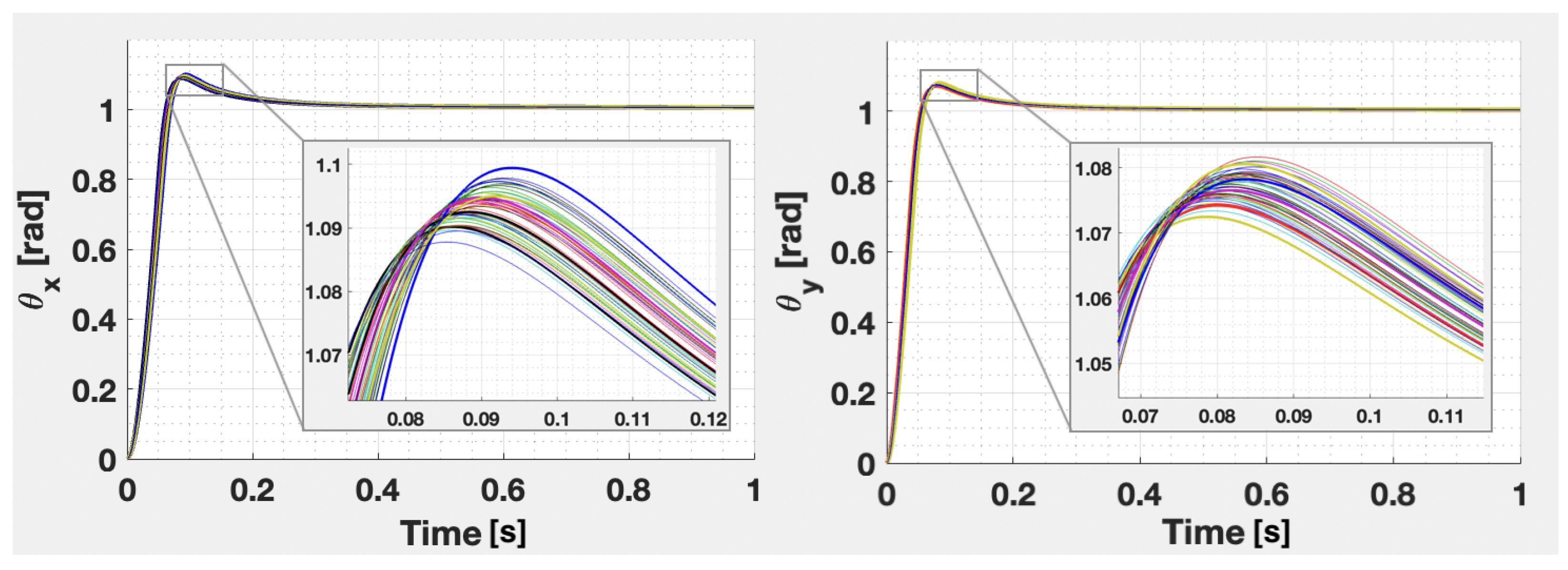
As mentioned in the theoretical part, in order to formulate the control problem of finding the PI-P cascade structure for each axis subsystem, it is necessary to augment the plant model with two extra states. The extended state-space model used is:
G ¯ δ ( s ) : ω ˙ x ( t ) θ ˙ x ( t ) z ˙ x ( t ) ω ˙ y ( t ) θ ˙ y ( t ) z ˙ y ( t ) θ x ( t ) θ y ( t ) = 40.85 0 0 0 0 0 1054 26.65 1 0 0 0 0 0 0 0 0 1 0 0 0 0 0 0 0 0 0 87.81 0 0 24.46 2188 0 0 0 1 0 0 0 0 0 0 0 0 1 0 0 0 0 1 0 0 0 0 0 0 0 0 0 0 1 0 0 0 ω x ( t ) θ x ( t ) z x ( t ) ω y ( t ) θ y ( t ) z y ( t ) u x ( t ) u y ( t ) .
Moreover, for the matrices corresponding to the DNLDI system in (14), A, B u , B d , C v , D v u , D v d , C y , D y u and D y d , the nominal values from Table 1 are used, along with the following terms for the uncertainties:
r T M x = 0.0024 ; r T M y = 0.0011 ; r K M x = 2.5802 ; r K M y = 2.4917 ; r K x y = 2.6650 ; r K y x = 2.4460 .
The performances for the closed loop system imposed through the D ( α , θ ) -region are:
  • A settling time t s 0.2 [ s e c ] , imposed using the corresponding vertical strip parameter α = 20 .
  • A very small overshoot, tending to zero, imposed by the conic region corresponding parameter θ = 0.01 .
  • The command signal allowed values u x , u y 1 , 1 , imposed by the corresponding LMI, having the initial conditions in the ellipsoid described using Q = I 6 .
As such, one LMI using the DNLDI form of the system is necessary for the settling time constraints, while for imposing the maximum overshoot, 32 LMIs are necessary. Considering the input saturation, the final problem involves finding a common solution to the 35 LMIs. Using the LMI Solver from MATLAB’s Robust Control Toolbox [28], a feasible solution has been successfully found:
P = 10 3 × 2.4209 0.0835 0.0031 0 0 0 0.0835 0.0031 0.0001 0 0 0 0.0031 0.0001 0.00004 0 0 0 0 0 0 1.1275 0.0249 0.0007 0 0 0 0.0249 0.0007 0.00002 0 0 0 0.0007 0.00002 0.00007 ,
Z = 0.0453 0.9385 0.0395 0 0 0 0 0 0 0.1431 0.4835 0.0149 ,
which leads to the following state-feedback matrix:
K = 0.8719 47.9103 616.4164 0 0 0 0 0 0 0.4557 33.7512 497.9665 .
Using the equivalence between the gains obtained for the state-feedback controller and the gains needed for the PI-P cascade control structure, we have:
P v ( x ) = 0.8719 , P p ( x ) = 54.9470 I p ( x ) = 706.9512 , P v ( y ) = 0.4557 , P p ( y ) = 74.0668 , I p ( y ) = 1092.8 .
Figure 2 shows the step responses obtained for the nominal models of each axis, along with 50 uncertain samples obtained with Monte Carlo simulations. As noticed, the imposed settling time for both axes is fulfilled, along with a zero steady-state error. The overshoot appears due to the transmission zero, as proved in Section 3.2. As such, a feedforward component is necessary to mitigate the transmission zero causing the overshoot and so that the performances imposed through the D ( α , θ ) -region are fully met. The values of the feedforward gains are:
K f f ( x ) = 54.947 and K f f ( y ) = 74.0668 .
The final configuration of the cascade control and feedforward component, together with the mutual effect between the axes and integrating the uncertainties, is depicted in Figure 3. The two resulting closed-loop systems have no transmission zeros and the eigenvalues obtained for the nominal state-space representation become:
Λ H 0 ( x ) = 904.85 , 33.72 , 21.29 ;
Λ H 0 ( y ) = 1013 , 50.6 , 21.3 .
The step responses for both nominal and uncertain systems of each axis obtained using the final control structure from Figure 3 are presented in Figure 4. As noticed, the settling time is robustly kept at t s 0.2 [s], with no detectable overshoot or steady-state error.
Next, we consider several numerical simulations obtained with the second proposed control structure, described in Figure 5. The inner P controller used for the speed loop should be designed considering the desired speed profile. For the purpose of this paper, we considered the same values K v ( x ) = 0.8719 and K v ( y ) = 0.4557 as in the previous structure in order to have a fair comparison.
For both axes we considered a bipositional relay with a hysteresis h = ± 0.5 and with the switching points at ± 0.05 . The resulting limit cycle for the X axis has the frequency ω o s c = 71.23 [rad/s] and the amplitude A o s c = 0.01 , while the resulting Y axis limit cycle has the frequency ω o s c = 69.38 [rad/s] and the amplitude A o s c = 0.01 . Because the amplitudes of both limit cycles are the same, the equivalent gains will be equal for both axes:
K e q ( x ) = K e q ( y ) = 63.662 .
The resulting time constants of the outer fractional-order integral-derivative controllers presented in (31) are T 1 ( x ) = 0.01 [s] and T 1 ( y ) = 9.21 × 10 4 [s]. By imposing the phase margin γ = 13 π 30 , the resulting fractional orders of both controllers are λ I ( x ) = λ I ( y ) = 0.133 . Moreover, to ensure ω g c = ω o s c , the controllers’ gains are K I ( x ) = 112.1283 and K I ( y ) = 111.8148 . As such, the outer controllers are:
H F O I D ( x ) ( s ) = 112.1283 0.01 s + 1 s 0.133 and H F O I D ( y ) ( s ) = 111.8148 9.21 · 10 4 s + 1 s 0.133 .
For the numerical results, the F O I D controllers has been simulated using MATLAB’s FOMCON toolbox [29]. The approximation order of the fractional-order elements has been set to 5, while the frequency range is [ 0.1 , 10 4 ] [rad/s]. The performance of the closed-loop systems is illustrated in Figure 6. As noticed, the value of the settling time is t s 0.2 [s], comparable to the value obtained using the previous structure, and there is no steady-state error. However, due to the lack of coupling consideration between the axes, a small overshoot σ 5 % appears, being the main limitation of the proposed method.
Moreover, the fractional-order ID controller requires an approximation for the numerical implementation, which cannot be considered on the equipment described in [27] and whose model has been considered in the current paper.

6. Discussions

The comparison between the two proposed methods should be on even grounds, as both ensure zero steady-state error and comprise of four degrees of freedom. Regarding the time-domain performances, the settling time values are similar, with an average value of 0.22 [s] for both axes with the first method, having the values between 0.215 [s] and 0.225 [s], while with the second method, the settling time has an average value of 0.185 [s], varying between 0.17 [s] and 0.2 [s]. Moreover, the second method presents a smaller rise time of ≈0.07 [s] against to the first method where the rise time is ≈0.12 [s]. The overshoot has been imposed to be 0 in the first method, while using the second method the resulting overshoot is ≈9.5 [%] for the X axis and ≈7.5 [%] for the Y axis, varying between 8.5 [ % ] and 10 [ % ] for the X axis and between 7 [ % ] and 8 [ % ] for the Y axis. Regarding the implementability, the first structure manages to deal with the limitations imposed by the control structure given by the MC206X Motion Coordinator, which provides five servo gains for control that allow the design of a P I D controller for the outer position loop, a P controller for the inner angular speed loop and a feedforward angular speed gain [27]. As such, regarding the implementability of the proposed control laws, the F O I D regulator cannot be implemented on a generic industrial controller where the structure could be fixed, as in our case.
Comparing the proposed methods with the available results in the literature, the first method presents a set of improvements against the similar method proposed in [25], where the uncertainties and the command signal limitations have not been considered, while the coupling between axes has been studied as a disturbance and only the capacity of globally rejecting such disturbances has been analyzed. Moreover, against the second paper which has been extended here, the problem of designing a F O I D controller for each axis considering the positional systems has been treated in the current paper, compared to [17], where only a single axis angular velocity control system has been treated. The overshoot presented using the second controller can be justified by the lack of consideration of the interconnections between the axes, but the approximation of the fractional-order element could also represent a problem. As noticed in other available research papers, the problem of a small overshoot appears even in the case of a single axis position system, as in [14,15,16]. However, the great advantage of the second method consists in being an autotuning method which manages to fulfill the vast majority of constraints imposed by such a problem: fast response with zero steady-state error.
As future work, we propose to investigate the possibility to mitigate the small overshoot presented in the case of using the F O I D controller by adding an extra degree of freedom such that the coupling between axes can also be removed. Moreover, a possible extension will be to add both control structures in the μ -synthesis control framework by considering the possibility to integrate the fractional-order element into the Robust Control Framework, starting from the ideas underlined in [19,20]. Additionally, another research direction will be the possibility to develop a graphical tuning method for such a system having a fractional-order model instead of an integer-order one, as in [21,22].

7. Conclusions

The current paper presents two design techniques for a two-axis positional-based mechatronic system. The first technique converts the well-known full state-feedback control structure into a cascade structure having a P controller on the inner loop and a PI controller on the outer loop. The state-feedback matrix has been computed based on the solution of an LMI-based problem in which a set of performances have been imposed by describing a D -region where the closed-loop poles will be placed, along with an extra condition to overcome the saturation effect which appears on both command signals. The results show that the settling time requirements are fulfilled, having an average value of 0.22 [s] for X axis and 0.175 [s] for Y axis, with no steady state-error, but with a small overshoot caused by a transmission zero. This transmission zero effect has also been canceled using a feedforward gain for each axis, leading to an average value of the settling time of ≈0.2 [s] for each axis, as imposed. Moreover, a great advantage of this method compared to the classical LQR scheme, as part of an extended range of optimal-control based control laws, is the ability to impose the regional location of the closed-loop system poles in order to obtain specific time-domain performances and counteract uncertainties.
The second technique presents a methodology to design a similar control structure, with two modifications: the feedforward gain has been removed, and the outer PI controller has been replaced with a F O I D controller designed by bringing the system to the limit cycle using a relay-type nonlinearity. However, the numerical results reveal one issue with this approach: the overshoot appears due to the design procedure of the outer controller which does not consider the coupling between the axes. The settling time has similar values in both control structures, with no steady-state error, but the first control structure presents no overshoot, while the second structure induces a small overshoot. As such, based on our findings, the LMI-based controller is suitable for this particular problem. Regarding the robustness, as illustrated in the previous section, the uncertainties do not significantly affect the imposed performances in both cases. Moreover, the method presents the advantage of being an autotuning one.

Author Contributions

Conceptualization, D.M. and V.M.; methodology, V.M.; software, V.M. and D.M.; validation, M.Ş. and P.D.; formal analysis, D.M. and P.D.; investigation, V.M.; resources, D.M.; data curation, M.Ş. and D.M.; writing—original draft preparation, D.M., V.M. and M.Ş.; writing—review and editing, M.Ş., D.M. and P.D.; visualization, P.D.; supervision, P.D.; project administration, D.M.; funding acquisition, P.D. All authors have read and agreed to the published version of the manuscript.

Funding

This paper was financially supported by the Project “Entrepreneurial competences and excellence research in doctoral and postdoctoral programs—ANTREDOC”, co-funded by the European Social Fund financing agreement no. 56437/24.07.2019.

Conflicts of Interest

The authors declare no conflict of interest.

Abbreviations

The following abbreviations are used in this manuscript:
ABCArtificial Bee Colony
CNCComputer Numerical Control
DNLDIDiagonal Norm-Bound Linear Differential Inclusion
FO-IDFractional-Order Integral-Derivative
FO-PIDFractional-Order Proportional-Integral-Derivative
LDILinear Differential Inclusion
LMILinear Matrix Inequality
LQGLinear-Quadratic-Gaussian
LQRLinear-Quadratic-Regulator
MIMOMultiple-Inputs and Multiple-Outputs
PIDProportional Integral Derivative
PLDIPolytopic Linear Differential Inclusion
PWMPulse Width Modulation
List of Symbols
S n + The set of symmetric and positive definite matrices of order n
ω x , ω y Angular speed for X and Y axes, respectively
θ x , θ y Angular position for X and Y axes, respectively
u x , u y Command signal for X and Y axes, respectively
θ x , θ y Angular position’s reference for X and Y axes, respectively
u x , u y Command signal for X and Y axes, respectively
z x , z y Additional states resulting after augmentation
T M x , T M y Time constant of the subsystem u ω for X and Y axes, respectively
K M x , K M y Gain factor of the subsystem u ω for X and Y axes, respectively
K x y , K y x Gain factor representing the interconnection between X and Y axes
c ( n ) The nominal value of an uncertain parameter c
d c The disturbance input corresponding to an uncertain parameter c
v c The disturbance output corresponding to an uncertain parameter c
c ̲ , c ¯ Lower and upper bound of an uncertain parameter c
P v ( x ) , P v ( y ) The resulting inner loop controllers’ parameters for both X and Y axes, respectively
P p ( x ) , I p ( x ) , P p ( y ) , I p ( y ) The resulting outer loop controllers’ parameters for both X and Y axes, respectively
K f f ( x ) , K f f ( y ) The feedforward gains for both X and Y axes, respectively
T 1 ( x ) , T 1 ( y ) Time constant of the outer F O I D controller for both X and Y axes, respectively
λ I ( x ) , λ I ( y ) Fractional order of the outer F O I D controller for both X and Y axes, respectively
K I ( x ) , K I ( y ) The gain of the outer F O I D controller for both X and Y axes, respectively

References

  1. Lee, T.H.; Liang, W.; de Silva, C.W.; Tan, K.K. Force and Position Control of Mechatronic Systems—Design and Applications in Medical Devices; Springer Nature: Cham, Switzerland, 2021. [Google Scholar]
  2. Chilali, M.; Gahinet, P. H Design with Pole Placement Constraints: An LMI Appproach. IEEE Trans. Autom. Control 1996, 41, 358–367. [Google Scholar] [CrossRef]
  3. Boyd, S.; El Ghaoui, L.; Feron, E.; Balakrishnan, V. Linear Matrix Inequalities in System and Control Theory; SIAM Studies in Applied Mathematics: Philadelphia, PA, USA, 1994. [Google Scholar]
  4. Assawinchaichote, V.; Nguang, S.K. H Fuzzy Control Design For Nonlinear Singularly Perturbed Systems with Pole Placement Constraints: An LMI Approach. IEEE Trans. Syst. Man Cybern. Part B (Cybern.) 2004, 34, 579–588. [Google Scholar] [CrossRef] [PubMed]
  5. Tarbouriech, S.; Queinnec, I.; Calliero, T.R.; Peres, P.L.D. Control design for bilinear systems with a guaranteed region of stability: An LMI-based approach. In Proceedings of the 17th Mediterranean Conference on Control and Automation, Thessaloniki, Greece, 24–26 June 2009; pp. 809–814. [Google Scholar]
  6. Sloth, C.; Esbensen, T.; Niss, M.O.K.; Stoustrup, J.; Odgaard, P.F. Robust LMI-based control of wind turbines with parametric uncertainties. In Proceedings of the 2009 IEEE Control Applications (CCA) & Intelligent Control (ISIC), St. Petersburg, Russia, 8–10 July 2009; pp. 776–781. [Google Scholar]
  7. Redondo, J.P.; Boada, B.L.; Díaz, V. LMI-Based H Controller of Vehicle Roll Stability Control Systems with Input and Output Delays. Sensors 2021, 21, 7850. [Google Scholar] [CrossRef] [PubMed]
  8. Guerrero-Sánchez, M.-E.; Hernández-González, O.; Lozano, R.; García-Beltrán, C.-D.; Valencia-Palomo, G.; López-Estrada, F.-R. Energy-Based Control and LMI-Based Control for a Quadrotor Transporting a Payload. Mathematics 2019, 7, 1090. [Google Scholar] [CrossRef] [Green Version]
  9. Olalla, C.; Leyva, R.; El Aroudi, A.; Queinnec, I. Robust LQR control for PWM converters: An LMI approach. IEEE Trans. Ind. Electron. 2009, 56, 2548–2558. [Google Scholar] [CrossRef]
  10. Daher, F.A.; Stoustrup, J. Robust structured control design via LMI optimization. IFAC Proc. 2011, 44, 7933–7938. [Google Scholar]
  11. Da Silva, L.R.T.; de Campos, L.A.H.; Potts, A.S. Robust Control for Helicopters Performance Improvement: An LMI Approach. J. Aerosp. Technol. Manag. 2020, 12, e3620. [Google Scholar] [CrossRef]
  12. Cocetti, M.; Donnarumma, S.; De Pascali, L.; Ragni, M.; Biral, F.; Panizzolo, F.; Rinaldi, P.P.; Sassaro, A.; Zaccarian, L. Hybrid nonovershooting set-point pressure regulation for a wet clutch. IEEE/ASME Trans. Mechatron. 2020, 25, 1276–1287. [Google Scholar] [CrossRef]
  13. Lino, P.; Maione, G. Fractional-order controllers for mechatronics and automotive applications. In Handbook of Fractional Calculus with Applications—Volume 6: Applications in Control; De Gruyter: Berlin, Germany, 2019; pp. 267–292. [Google Scholar]
  14. Dulf, E.-H.; Șușcă, M.; Kovács, L. Novel Optimum Magnitude Based Fractional Order Controller Design Method. IFAC-PapersOnLine 2018, 51, 912–917. [Google Scholar] [CrossRef]
  15. Rahman, M.Z.U.; Leiva, V.; Martin-Barreiro, C.; Mahmood, I.; Usman, M.; Rizwan, M. Fractional Transformation-Based Intelligent H-Infinity Controller of a Direct Current Servo Motor. Fractal Fract. 2023, 7, 29. [Google Scholar] [CrossRef]
  16. Dulf, E.-H. Simplified Fractional Order Controller Design Algorithm. Mathematics 2019, 7, 1166. [Google Scholar] [CrossRef]
  17. Duma, R.; Dobra, P.; Trusca, M. Embedded application of fractional order control. Electron. Lett. 2012, 48, 1526–1528. [Google Scholar] [CrossRef]
  18. Mihaly, V.; Şuşcă, M.; Morar, D.; Stănese, M.; Dobra, P. μ-Synthesis for Fractional-Order Robust Controllers. Mathematics 2021, 9, 911. [Google Scholar] [CrossRef]
  19. Mihaly, V.; Şuşcă, M.; Dulf, E.H. μ-Synthesis FO-PID for Twin Rotor Aerodynamic System. Mathematics 2021, 9, 2504. [Google Scholar] [CrossRef]
  20. Mihaly, V.; Şuşcă, M.; Dulf, E.H.; Dobra, P. Approximating the Fractional-Order Element for the Robust Control Framework. In Proceedings of the 2022 American Control Conference, Atlanta, GA, USA, 8–10 June 2022; pp. 1151–1157. [Google Scholar]
  21. Ghorbani, M.; Tepljakov, A.; Petlenkov, E. Stabilizing region of fractional-order proportional integral derivative controllers for interval fractional-order plants. Trans. Inst. Meas. Control 2022, 45, 546–556. [Google Scholar] [CrossRef]
  22. Zheng, S.; Tang, X.; Song, B. A graphical tuning method of fractional order proportional integral derivative controllers for interval fractional order plant. J. Process. Control 2014, 24, 1691–1709. [Google Scholar] [CrossRef]
  23. Sławomir, M. Comparison of automatically tuned cascade control systems of servo-drives for numerically controlled machine tools. Elektron. Elektrotechnika 2014, 20, 16–23. [Google Scholar]
  24. Morar, D.; Dobra, P. Optimal LQR weight matrices selection for a CNC machine controller. In Proceedings of the 2021 23rd International Conference on Control Systems and Computer Science (CSCS), Bucharest, Romania, 26–28 May 2021. [Google Scholar]
  25. Morar, D.; Mihaly, V.; Şuşcă, M.; Dobra, M. LMI Conditions for CNC Cascade Controller Design - A State Feedback Approach. In Proceedings of the 2022 IEEE International Conference on Automation, Quality and Testing, Robotics (AQTR), Cluj-Napoca, Romania, 19–21 May 2022; pp. 1–6. [Google Scholar]
  26. Shaul, G.; Jury, E. A general theory for matrix root-clustering in subregions of the complex plane. IEEE Trans. Autom. Control 1981, 26, 853–863. [Google Scholar]
  27. Morar, D. Advanced Control Techniques for CNC Machines. Ph.D. Thesis, Technical University of Cluj-Napoca, Cluj-Napoca, Romania, 2022. [Google Scholar]
  28. Balas, G.; Chiang, R.; Packard, A.; Safonov, M. Robust Control Toolbox—User’s Guide; The MathWorks: Natick, MA, USA, 2020. [Google Scholar]
  29. Tepljakov, A. FOMCON Toolbox for MATLAB; GitHub: San Francisco, CA, USA, 2022; Available online: https://github.com/extall/fomcon-matlab/releases/tag/v1.50.4 (accessed on 3 December 2022).
Figure 1. Single-axis mechanical model for the case study in (a), with the brushless DC motor characteristics in (b), used for system identification and control.
Fractalfract 07 00122 g001
Figure 2. The step responses of the nominal (red) closed-loop system, along with 50 Monte Carlo simulations (blue) for X axis (left) and Y axis (right), without considering the feedforward component.
Fractalfract 07 00122 g002
Figure 3. Cascade and feedforward configuration for the MIMO system.
Fractalfract 07 00122 g003
Figure 4. The step responses of the nominal closed-loop system, along with 50 Monte Carlo simulations for X axis (left) and Y axis (right), obtained by adding the feedforward component.
Fractalfract 07 00122 g004
Figure 5. Closed-loop control structure for the two-axis positional mechatronic system having a P controller on the inner speed loop, and a F O I D controller on the outer position loop, the switching element being used to commute between the controller (working mode) and the relay (design mode).
Fractalfract 07 00122 g005
Figure 6. The step responses of the nominal closed-loop system, along with 50 Monte Carlo simulations for X axis (left) and Y axis (right).
Fractalfract 07 00122 g006
Table 1. Nominal values of the system’s parameters, along with their uncertainty ranges.
ParameterNominal ValuePercentageParameterNominal ValuePercentage
T M x 0.0245 ± 10 % K M x 25.8017 ± 10 %
T M y 0.0114 ± 10 % K M y 24.9174 ± 10 %
K x y 26.65 ± 10 % K y x 24.46 ± 10 %
Disclaimer/Publisher’s Note: The statements, opinions and data contained in all publications are solely those of the individual author(s) and contributor(s) and not of MDPI and/or the editor(s). MDPI and/or the editor(s) disclaim responsibility for any injury to people or property resulting from any ideas, methods, instructions or products referred to in the content.

