

Mandelbrot and Julia Sets of Transcendental Functions Using Picard–Thakur Iteration


Abstract
:1. Introduction
2. Preliminaries
3. Main Results
3.1. Escape Criterion for
3.2. Escape Criterion for
4. Algorithms
| Algorithm 1 The Mandelbrot set. |
| 1. Setup: Take a complex number Initialize the variables , , Set 2. Iterate: where or , , . 3. Stop: Escape radius 4. Count: The number of iterations undertaken to escape. 5. Color: Assign a color to each point based on the number of iterations needed to escape. |
| Algorithm 2 The Julia set. |
| 1. Setup: Take a complex number Initialize the variables , , Consider first iteration 2. Iterate: where or , , . 3. Stop: Escape radius 4. Count: Number of iterations undertaken to escape. 5. Color: Based on the number of iterations needed to escape. |
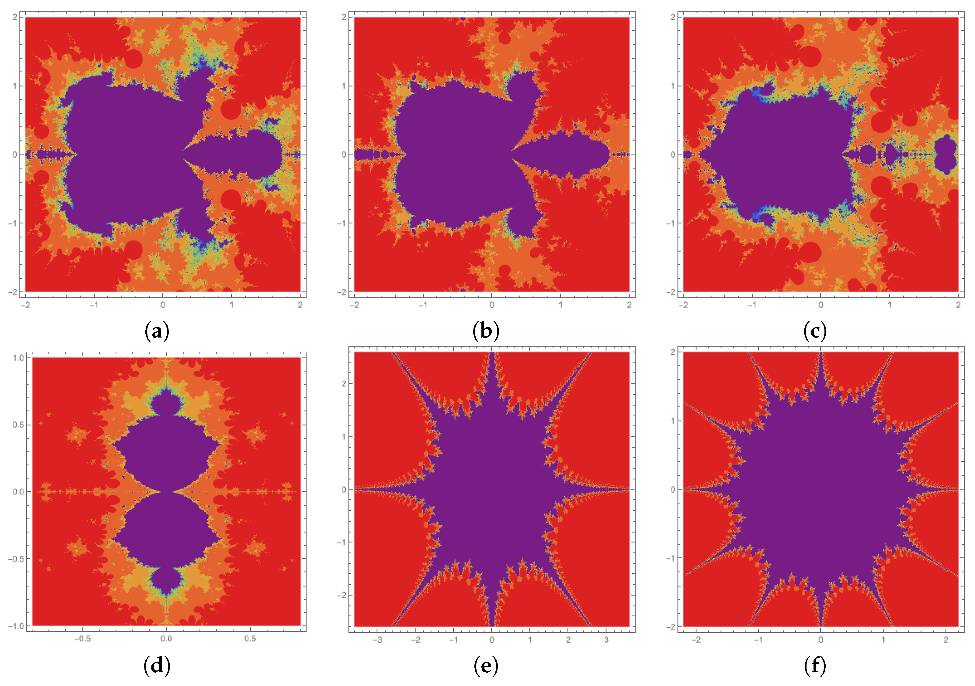
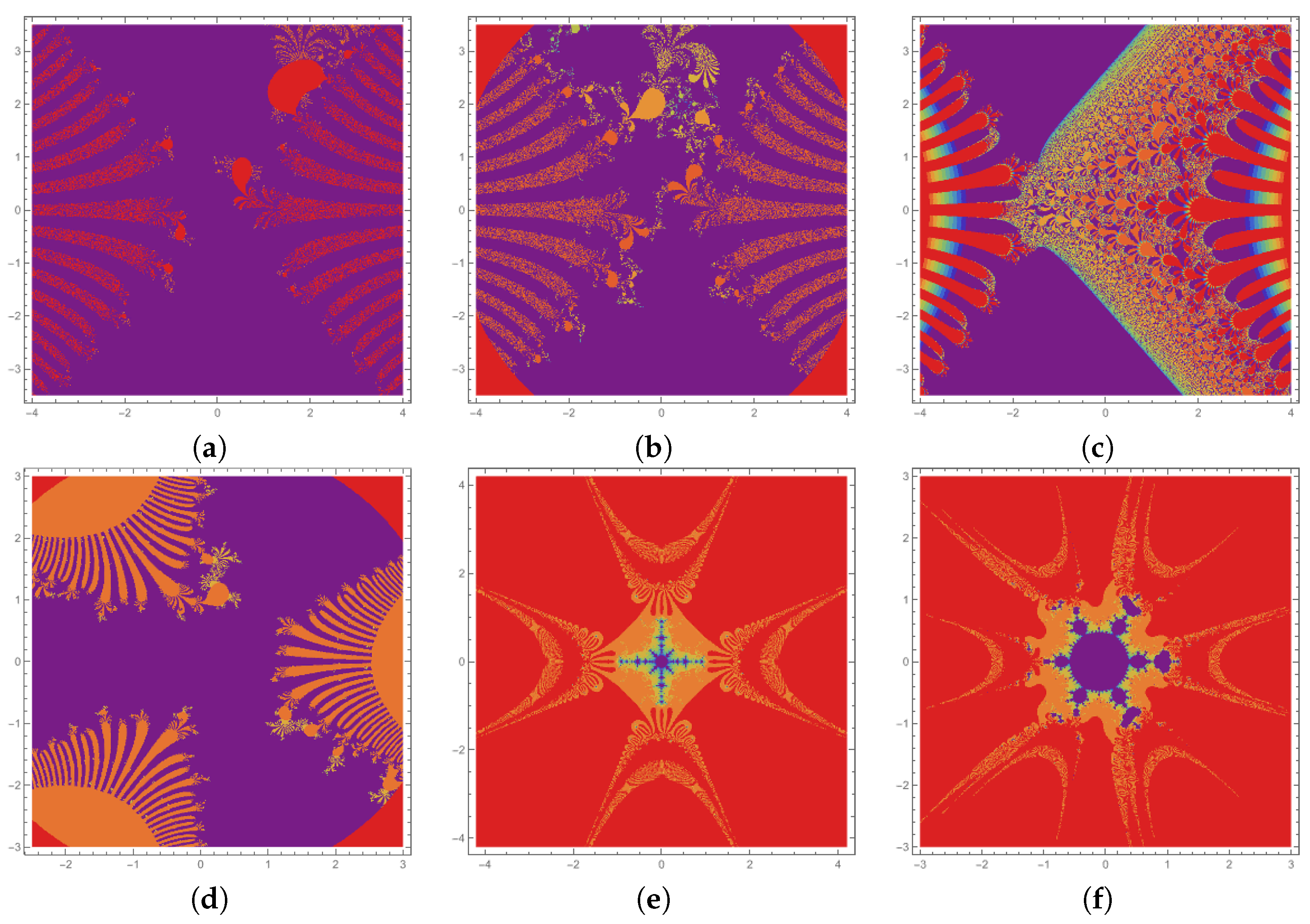
4.1. Mandelbrot Sets for
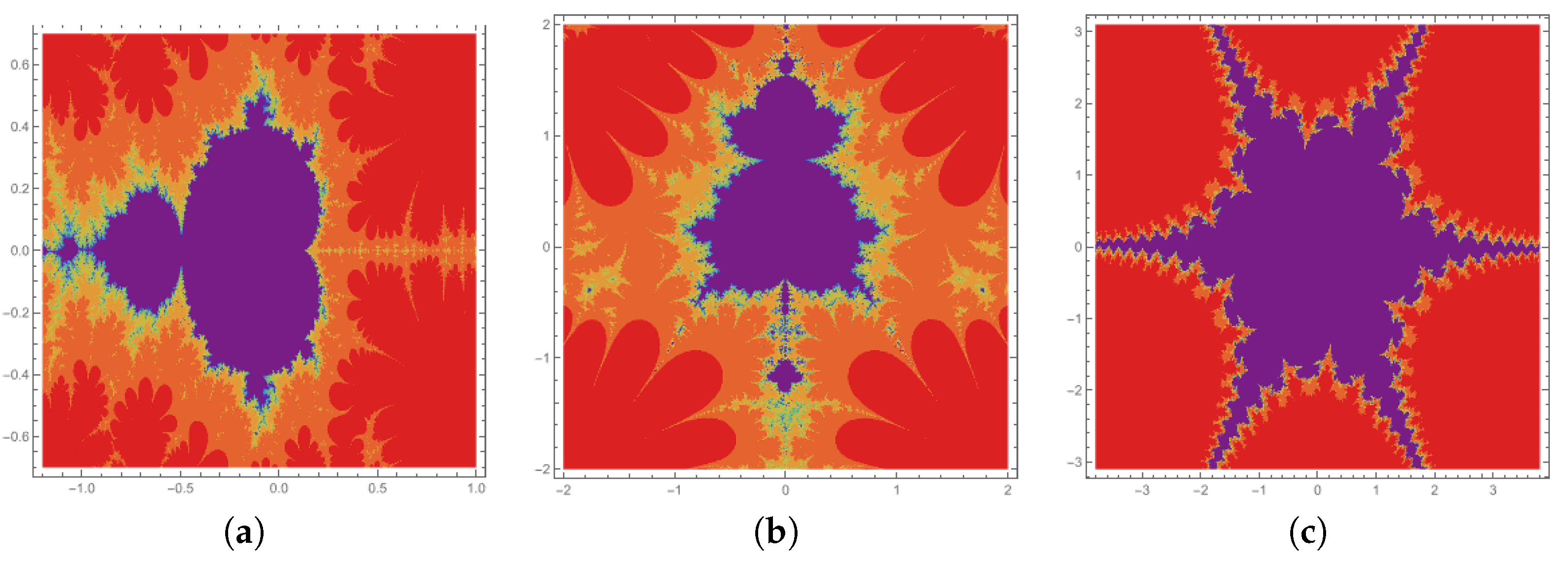
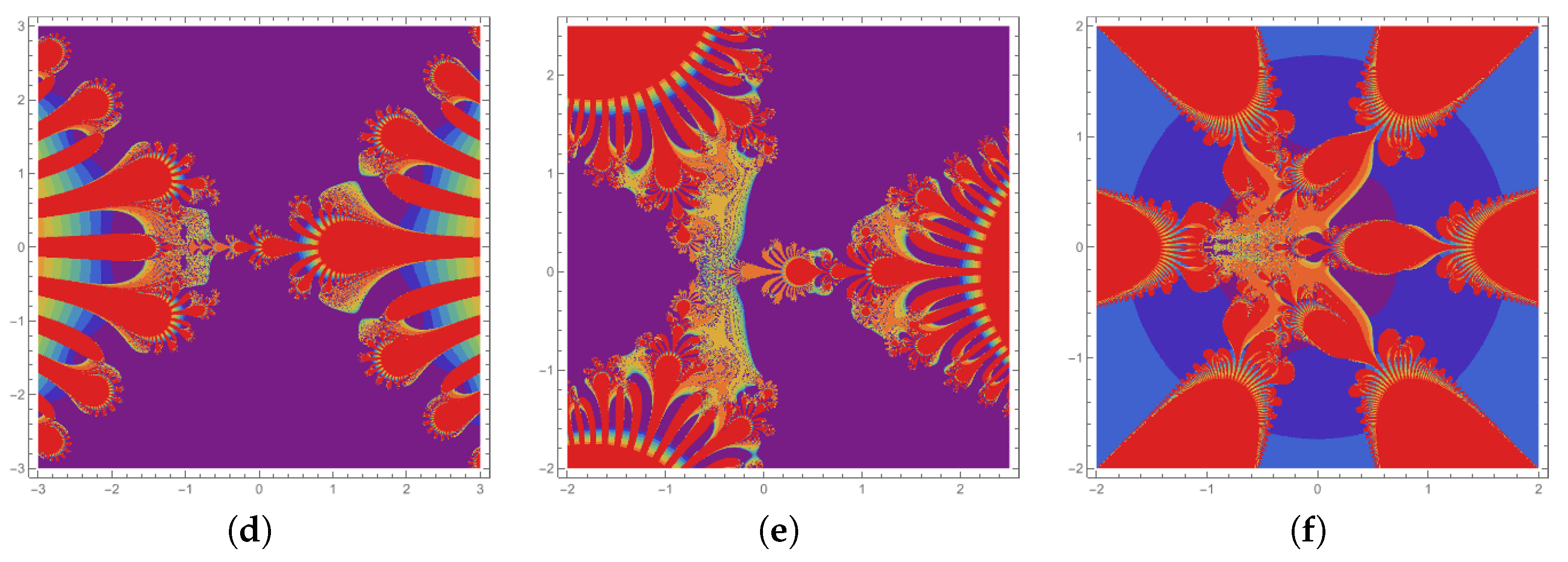
4.2. Mandelbrot Sets for
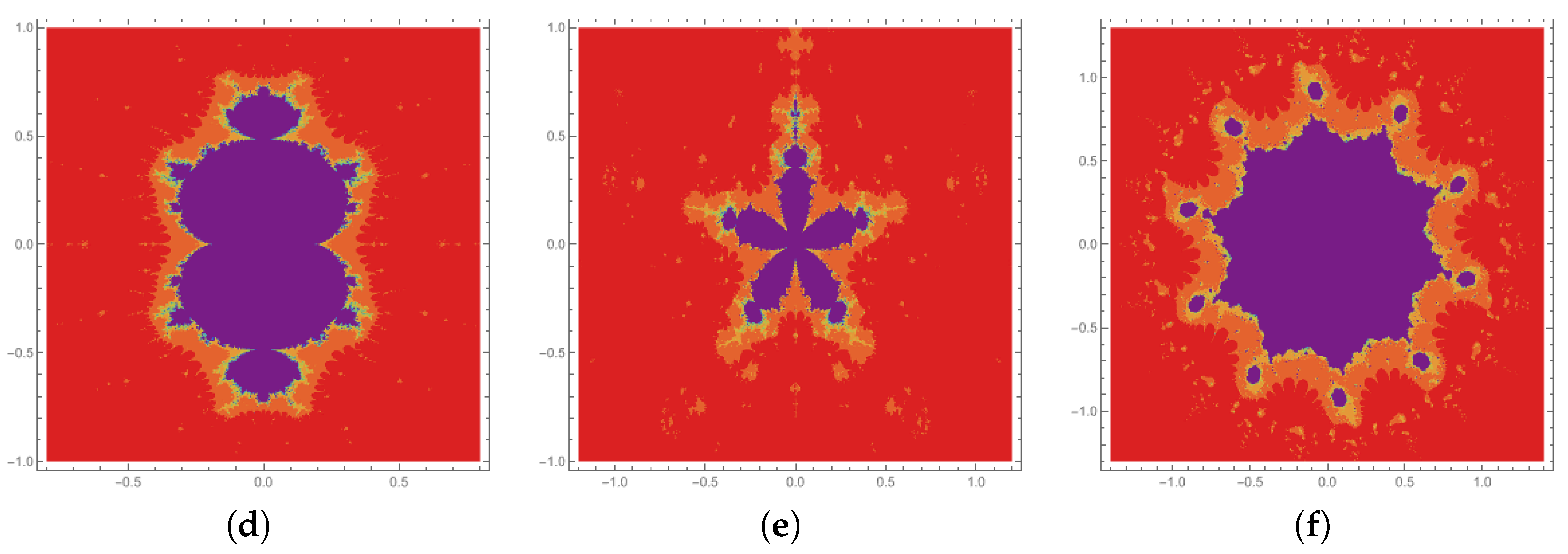
4.3. Julia Sets for
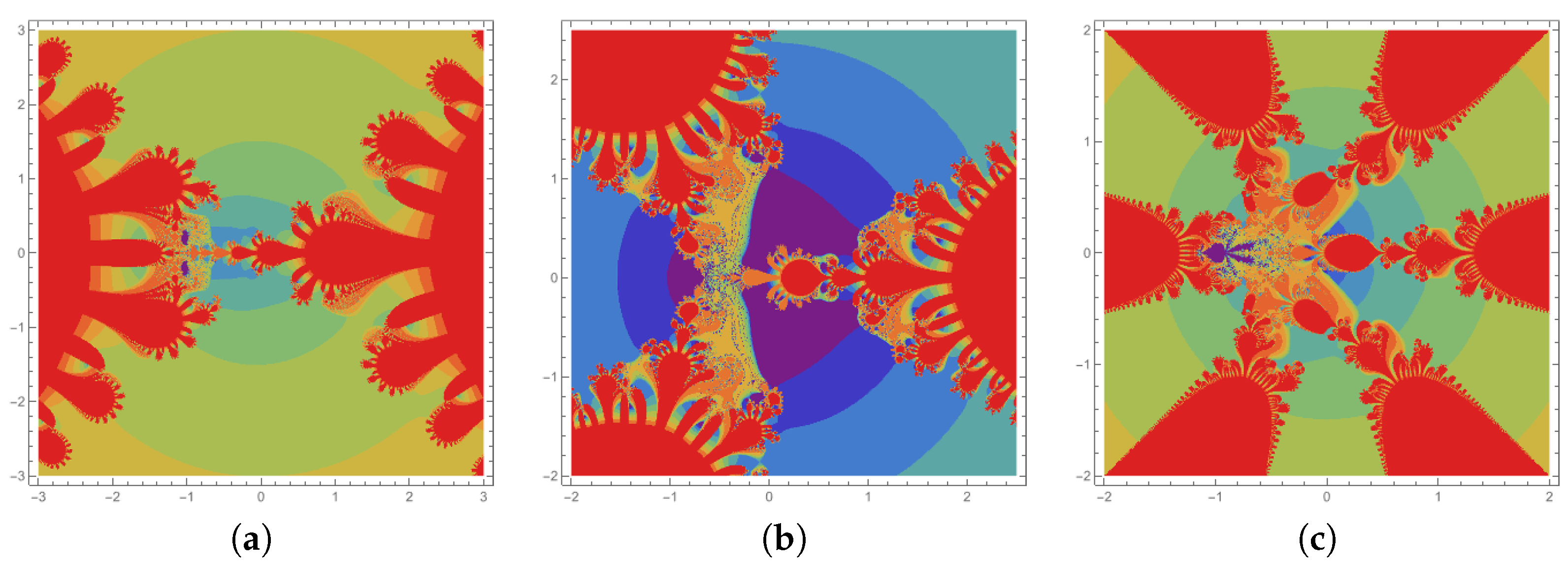
4.4. Julia Sets for
5. Conclusions
Author Contributions
Funding
Data Availability Statement
Conflicts of Interest
Appendix A
Appendix A.1. Source Program to Generate the Julia Sets
Appendix A.2. Source Program to Generate Mandelbrot Sets
References
- Mandelbrot, B.B. Les Objects Fractals: Forme, Hasard et Dimension; Flammarion: Paris, France, 1975; Volume 17. [Google Scholar]
- Julia, G. Sur l’iteration des functions rationnelles. J. Math. Pures Appl. 1918, 8, 737–747. [Google Scholar]
- Rani, M.; Kumar, V. Superior Julia set. Res. Math. Educ. 2004, 8, 261–277. [Google Scholar]
- Rani, M.; Kumar, V. Superior Mandelbrot set. Res. Math. Educ. 2004, 8, 279–291. [Google Scholar]
- Rani, M. Cubic superior Julia sets. In Proceedings of the European Computing Conference, Paris, France, 28–30 April 2011; pp. 80–84. [Google Scholar]
- Prasad, B.; Katiyar, K. Fractals via Ishikawa iteration. In Proceedings of the International Conference on Logic, Information, Control and Computation, Gandhigram, India, 25–27 February 2011; Springer: Berlin/Heidelberg, Germany, 2011; pp. 197–203. [Google Scholar]
- Ashish; Rani, M.; Chugh, R. Julia sets and Mandelbrot sets in Noor orbit. Appl. Math. Comput. 2014, 228, 615–631. [Google Scholar] [CrossRef]
- Abbas, M.; Iqbal, H.; De la Sen, M. Generation of Julia and Mandelbrot sets via fixed points. Symmetry 2020, 12, 86. [Google Scholar] [CrossRef]
- Tanveer, M.; Nazeer, W.; Gdawiec, K. New escape criteria for complex fractals generation in Jungck-CR orbit. Indian J. Pure Appl. Math. 2020, 51, 1285–1303. [Google Scholar] [CrossRef]
- Kang, S.M.; Nazeer, W.; Tanveer, M.; Shahid, A.A. New fixed point results for fractal generation in Jungck Noor orbit with s-convexity. J. Funct. Spaces 2015, 2015, 963016. [Google Scholar] [CrossRef]
- Goyal, K.; Prasad, B. Dynamics of iterative schemes for quadratic polynomial. AIP Conf. Proc. 2017, 1897, 020031. [Google Scholar]
- Nazeer, W.; Kang, S.M.; Tanveer, M.; Shahid, A.A. Fixed point results in the generation of Julia and Mandelbrot sets. J. Inequal. Appl. 2015, 2015, 298. [Google Scholar] [CrossRef]
- Kwun, Y.C.; Tanveer, M.; Nazeer, W.; Abbas, M.; Kang, S.M. Fractal generation in modified Jungck–S orbit. IEEE Access 2019, 7, 35060–35071. [Google Scholar] [CrossRef]
- Li, D.; Tanveer, M.; Nazeer, W.; Guo, X. Boundaries of filled julia sets in generalized Jungck Mann orbit. IEEE Access 2019, 7, 76859–76867. [Google Scholar] [CrossRef]
- Romera, M.; Pastor, G.; Alvarez, G.; Montoya, F. Growth in complex exponential dynamics. Comput. Graph. 2000, 24, 115–131. [Google Scholar] [CrossRef]
- Prasad, B.; Katiyar, K. Dynamics of Julia Sets for complex exponential functions. In Proceedings of the Mathematical Modelling and Scientific Computation: International Conference, ICMMSC 2012, Gandhigram, India, 16–18 March 2012; Springer: Berlin/Heidelberg, Germany, 2012; pp. 185–192. [Google Scholar]
- Prajapati, D.J.; Rawat, S.; Tomar, A.; Sajid, M.; Dimri, R.C. A brief study on Julia sets in the dynamics of entire transcendental function using Mann iterative scheme. Fractal Fract. 2022, 6, 397. [Google Scholar] [CrossRef]
- Qi, H.; Tanveer, M.; Nazeer, W.; Chu, Y. Fixed point results for fractal generation of complex polynomials involving sine function via non-standard iterations. IEEE Access 2020, 8, 154301–154317. [Google Scholar] [CrossRef]
- Hamada, N.; Kharbat, F. Mandelbrot and Julia Sets of complex polynomials involving sine and cosine functions via Picard–Mann Orbit. Complex Anal. Oper. Theory 2023, 17, 13. [Google Scholar] [CrossRef]
- Tomar, A.; Kumar, V.; Rana, U.S.; Sajid, M. Fractals as Julia and Mandelbrot Sets of complex cosine functions via fixed point iterations. Symmetry 2023, 15, 478. [Google Scholar] [CrossRef]
- Tassaddiq, A.; Tanveer, M.; Azhar, M.; Arshad, M.; Lakhani, F. Escape criteria for generating fractals of complex functions using DK-iterative scheme. Fractal Fract. 2023, 7, 76. [Google Scholar] [CrossRef]
- Tanveer, M.; Nazeer, W.; Gdawiec, K. On the Mandelbrot set of zp + log ct via the Mann and Picard–Mann iterations. Math. Comput. Simul. 2023, 209, 184–204. [Google Scholar] [CrossRef]
- Alonso-Sanz, R. A glimpse of complex maps with memory. Complex Syst. 2013, 21, 269–282. [Google Scholar] [CrossRef]
- Cohen, N. Fractal antenna applications in wireless telecommunications. In Proceedings of the Professional Program Proceedings, Electronic Industries Forum of New England, Boston, MA, USA, 6–8 May 1997; IEEE: Piscataway, NJ, USA, 1997; pp. 43–49. [Google Scholar]
- Fisher, Y. Fractal image compression. Fractals 1994, 2, 347–361. [Google Scholar] [CrossRef]
- Sun, Y.; Chen, L.; Xu, R.; Kong, R. An image encryption algorithm utilizing Julia sets and Hilbert curves. PLoS ONE 2014, 9, e84655. [Google Scholar] [CrossRef] [PubMed]
- Hsü, K.J.; Hsü, A.J. Fractal geometry of music. Proc. Natl. Acad. Sci. USA 1990, 87, 938–941. [Google Scholar] [CrossRef] [PubMed]
- Devaney, R.L. A First Course in Chaotic Dynamical Systems: Theory and Experiment; Addison-Wesley: Boston, MA, USA, 1992. [Google Scholar]
- Jia, J.; Shabbir, K.; Ahmad, K.; Shah, N.A.; Botmart, T. Strong convergence of a new hybrid iterative scheme for nonexpansive mappings and applications. J. Funct. Spaces 2022, 2022, 4855173. [Google Scholar]


| Figure | r | a | b | |||||||
|---|---|---|---|---|---|---|---|---|---|---|
| Figure 1a | 2 | 0.8 | 0.5 | 0.7 | 0.7 | 0.4 | 0.4 | 0.2 | 0.2 | 0.2 |
| Figure 1b | 2 | 0.08 | 0.05 | 0.07 | 0.07 | 0.4 | 0.4 | 0.8 | 0.8 | 0.8 |
| Figure 1c | 2 | 0.8 | 0.5 | 0.7 | 0.7 | 1 | 0 | 0.2 | 0.2 | 0.2 |
| Figure 1d | 3 | 0.08 | 0.05 | 0.07 | 0.07 | 1.14 | 0.9 | 0.9 | 0.9 | 0.9 |
| Figure 1e | 4 | 0.08 | 0.05 | 0.07 | 0.07 | 0.0014 | 0.0009 | 0.009 | 0.009 | 0.009 |
| Figure 1f | 6 | 0.08 | 0.05 | 0.07 | 0.07 | 0.0014 | 0.0009 | 0.009 | 0.009 | 0.009 |
| Figure | r | a | b | |||||||
|---|---|---|---|---|---|---|---|---|---|---|
| Figure 2a | 2 | 0.08 | 0.05 | 0.07 | 0.07 | 2.02 + 0.002i | 0.002i | 0.9 | 0.9 | 0.8 |
| Figure 2b | 2 | 0.8 | 0.5 | 0.7 | 0.7 | 1.0002i | 0.009i | 0.002 | 0.002 | 0.002 |
| Figure 2c | 3 | 0.08 | 0.05 | 0.07 | 0.07 | 0.014i | 0.009i | 0.09 | 0.09 | 0.09 |
| Figure 2d | 3 | 0.08 | 0.05 | 0.07 | 0.07 | 3.14 + 0.005i | 0.09 | 0.9 | 0.9 | 0.9 |
| Figure 2e | 6 | 0.08 | 0.05 | 0.07 | 0.07 | 1.14i | 0.9 | 0.9 | 0.9 | 0.9 |
| Figure 2f | 11 | 0.01 | 0.01 | 0.01 | 0.01 | −1.14i | −0.9i | 0.002 | 0.004 | 0.006 |
| Figure | r | a | b | |||||||
|---|---|---|---|---|---|---|---|---|---|---|
| Figure 3a | 2 | 0.08 | 0.05 | 0.07 | 0.07 | 1.02 | 1.2 | 0.9 | 0.9 | 0.8 |
| Figure 3b | 3 | 0.08 | 0.05 | 0.07 | 0.07 | 1.02 | 1.2 | 0.2 | 0.2 | 0.2 |
| Figure 3c | 6 | 0.08 | 0.05 | 0.07 | 0.07 | 1.02 | 1.2 | 0.2 | 0.2 | 0.2 |
| Figure 3d | 2 | 0.000812 | 0.000575 | 0.000786 | 0.000775 | 1.02 | 1.2 | 0.9 | 0.9 | 0.8 |
| Figure 3e | 3 | 0.000812 | 0.000575 | 0.000786 | 0.000775 | 1.02 | 1.2 | 0.2 | 0.2 | 0.2 |
| Figure 3f | 6 | 0.000812 | 0.000575 | 0.000786 | 0.000775 | 1.02 | 1.2 | 0.2 | 0.2 | 0.2 |
| Figure | r | a | b | |||||||
|---|---|---|---|---|---|---|---|---|---|---|
| Figure 4a | 2 | 0.000814 | 0.000545 | 0.000721 | 0.000748 | 0.004i | 1.3 + 0.004i | 0.09 | 0.08 | 0.06 |
| Figure 4b | 3 | 0.000814 | 0.000545 | 0.000721 | 0.000748 | 0.004i | 1.3 + 0.004i | 0.09 | 0.08 | 0.06 |
| Figure 4c | 4 | 0.000814 | 0.000545 | 0.000721 | 0.000748 | 0.004i | 1.3 + 0.004i | 0.09 | 0.08 | 0.06 |
| Figure | r | a | b | c | |||||||
|---|---|---|---|---|---|---|---|---|---|---|---|
| Figure 5a | 2 | 0.06 | 0.07 | 0.08 | 0.09 | 1 | 0 | −0.007i | 0.01 | 0.02 | 0.03 |
| Figure 5b | 2 | 0.06 | 0.07 | 0.08 | 0.09 | 1 | 0.5 | −0.007i | 0.01 | 0.02 | 0.03 |
| Figure 5c | 2 | 0.06 | 0.07 | 0.08 | 0.09 | 1.7 | 0 | −0.007i | 0.01 | 0.02 | 0.03 |
| Figure 5d | 3 | 0.6 | 0.7 | 0.8 | 0.9 | 0.8 | 0.02 | 0.0007 − 0.0007i | 0.03 | 0.03 | 0.03 |
| Figure 5e | 3 | 0.6 | 0.7 | 0.8 | 0.9 | 0.8 | 0.02 | 0.0007 − 0.0007i | 0.5 | 0.5 | 0.5 |
| Figure 5f | 3 | 0.6 | 0.7 | 0.8 | 0.9 | 0.8 | 0.02 | 0.0007 − 0.0007i | 0.9 | 0.9 | 0.9 |
| Figure 5g | 4 | 0.6 | 0.7 | 0.8 | 0.9 | 0.2 | 1.2 | 0.0008888 | 0.07 | 0.05 | 0.08 |
| Figure 5h | 4 | 0.6 | 0.7 | 0.8 | 0.9 | 2.2 | 1.2 | −0.00088 − 0.00088i | 0.07 | 0.05 | 0.08 |
| Figure 5i | 8 | 0.6 | 0.7 | 0.8 | 0.9 | 1.2 | 1.2 | −0.0008i | 0.07 | 0.05 | 0.08 |
| Figure | r | a | b | c | |||||||
|---|---|---|---|---|---|---|---|---|---|---|---|
| Figure 6a | 2 | 0.5 | 0.7 | 0.4 | 0.7 | 1 | 0 | −0.5i | 0.5 | 0.7 | 0.7 |
| Figure 6b | 2 | 0.5 | 0.7 | 0.4 | 0.7 | 1 | 0 | −0.5i | 0.9 | 0.9 | 0.9 |
| Figure 6c | 2 | 0.000580 | 0.000745 | 0.000456 | 0.000714 | 0.05 | 1.2 | 0.45 − 0.08i | 0.5 | 0.7 | 0.9 |
| Figure 6d | 3 | 0.7 | 0.9 | 0.3 | 0.5 | −1 | 0.001 | 0.4i | 0.4 | 0.4 | 0.4 |
| Figure 6e | 4 | 0.7 | 0.9 | 0.3 | 0.5 | −1 | 0.0001 | 2 | 0.0001 | 0.0001 | 0.0001 |
| Figure 6f | 6 | 0.07 | 0.09 | 0.03 | 0.05 | −1 | 0.0001 | 2 | 0.09 | 0.09 | 0.09 |
Disclaimer/Publisher’s Note: The statements, opinions and data contained in all publications are solely those of the individual author(s) and contributor(s) and not of MDPI and/or the editor(s). MDPI and/or the editor(s) disclaim responsibility for any injury to people or property resulting from any ideas, methods, instructions or products referred to in the content. |
© 2023 by the authors. Licensee MDPI, Basel, Switzerland. This article is an open access article distributed under the terms and conditions of the Creative Commons Attribution (CC BY) license (https://creativecommons.org/licenses/by/4.0/).
Share and Cite
Bhoria, A.; Panwar, A.; Sajid, M. Mandelbrot and Julia Sets of Transcendental Functions Using Picard–Thakur Iteration. Fractal Fract. 2023, 7, 768. https://doi.org/10.3390/fractalfract7100768
Bhoria A, Panwar A, Sajid M. Mandelbrot and Julia Sets of Transcendental Functions Using Picard–Thakur Iteration. Fractal and Fractional. 2023; 7(10):768. https://doi.org/10.3390/fractalfract7100768
Chicago/Turabian StyleBhoria, Ashish, Anju Panwar, and Mohammad Sajid. 2023. "Mandelbrot and Julia Sets of Transcendental Functions Using Picard–Thakur Iteration" Fractal and Fractional 7, no. 10: 768. https://doi.org/10.3390/fractalfract7100768