

Unraveling the Dynamics of Singular Stochastic Solitons in Stochastic Fractional Kuramoto–Sivashinsky Equation

 , and
, and 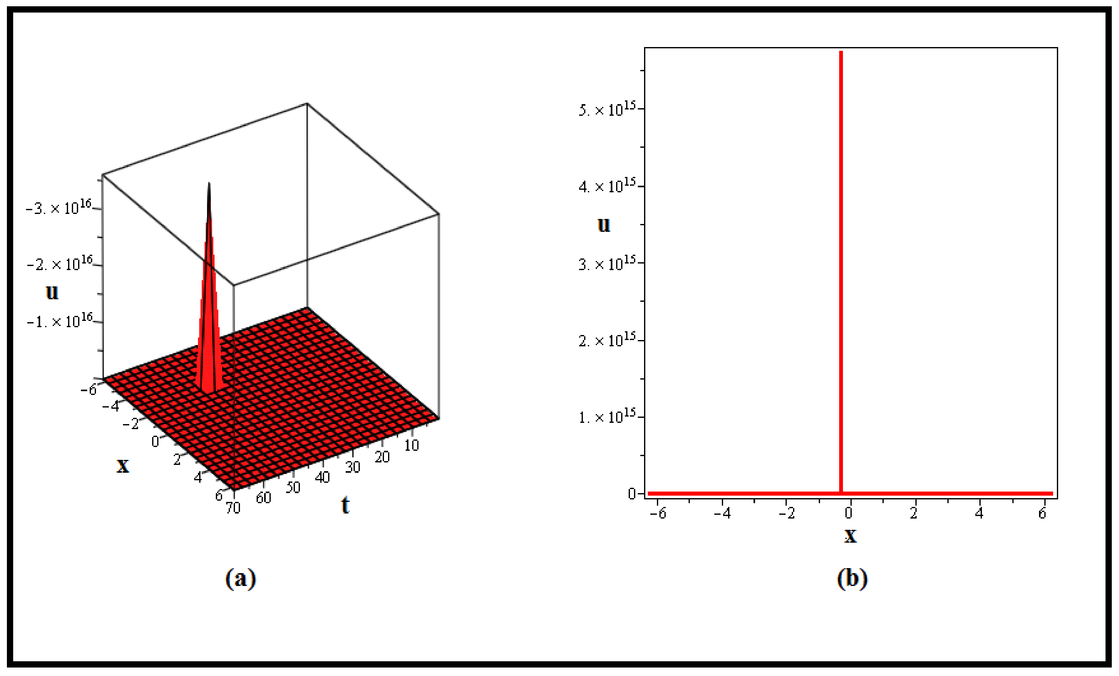
Abstract
:1. Introduction
2. Methodology and Resources
2.1. Brownian Motion
- ;
- is continuous function;
- is independent for ;
- has a Gaussian distribution with mean 0 and variance .
2.2. Conformable Fractional Derivative
2.3. The Working Mechanism of mEDAM
- First, , , ( can be written in many ways) is executed to turn (6) into a NODE of the form:where Y in (7) has derivatives with respect to . Equation (7) may occasionally be integrated once or more to obtain the integration’s constant.
- Then, we assume the following series form solution for (7):where are unknown constants to be found later, and is the general solution of the subsequent ODE.where and and c are invariables.
- The positive integer j present in (8) is called balance number, which is obtained by taking the homogeneous balance between the highest order derivative and the biggest nonlinear term in (7).
- Following that, we insert (8) into (7) or into the equation created by integrating (7), and we then compile all of the terms of that are in the same order and produce an expression in . A system of algebraic equations in and other parameters is produced by equating all the coefficients of the expression to zero using the concept of comparison of coefficients.
- To solve this set of algebraic equations, we use Maple-13 software.
- The soliton solutions to (6) are then explored by determining the unidentified coefficients and additional parameters and placing them in (8) together with the (general solution of (9)). The families of soliton solutions shown below may be produced using this generic solution of (9).
3. Wave Equation for SFKSE
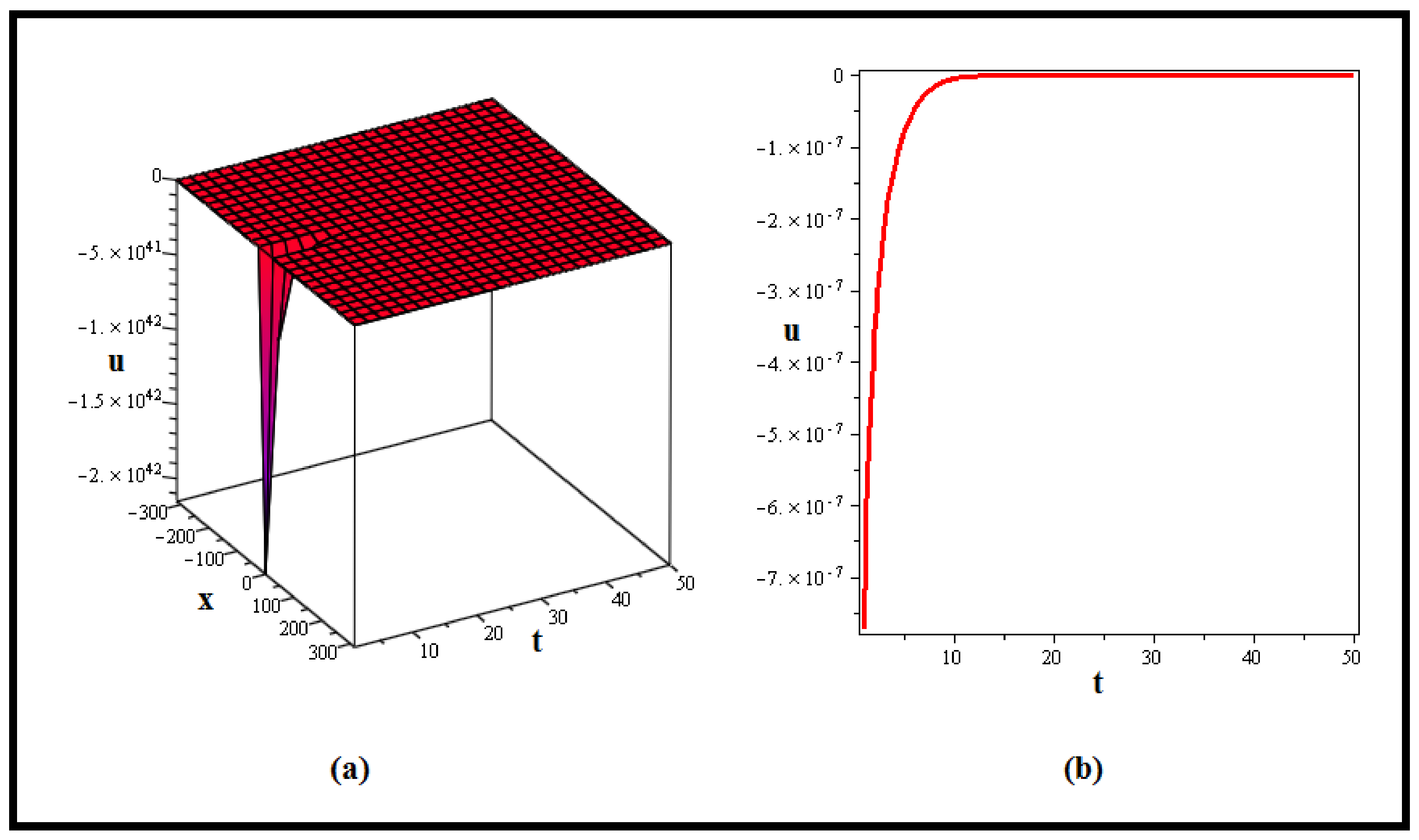
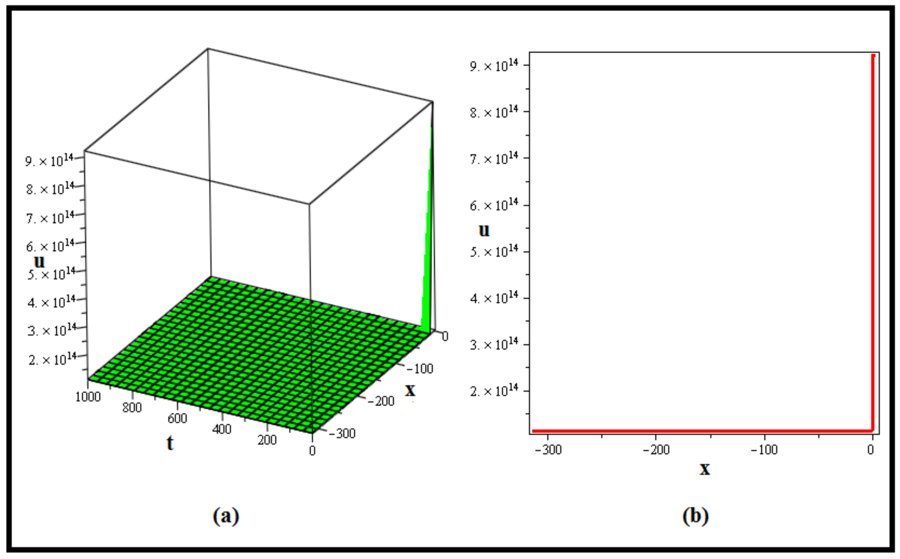
4. Stochastic Soliton Solutions
5. Discussion and Graphs
6. Conclusions
Author Contributions
Funding
Data Availability Statement
Acknowledgments
Conflicts of Interest
References
- Kamrani, M. Numerical solution of stochastic fractional differential equations. Numer. Algorithms 2015, 68, 81–93. [Google Scholar] [CrossRef]
- Mohammadi, F. Efficient Galerkin solution of stochastic fractional differential equations using second kind Chebyshev wavelets. Bol. Soc. Parana. Mat. 2017, 35, 195–215. [Google Scholar] [CrossRef]
- Abouagwa, M.; Li, J. Approximation properties for solutions to Itô–Doob stochastic fractional differential equations with non-Lipschitz coefficients. Stoch. Dyn. 2019, 19, 1950029. [Google Scholar] [CrossRef]
- Botmart, T.; Agarwal, R.P.; Naeem, M.; Khan, A. On the solution of fractional modified Boussinesq and approximate long wave equations with non-singular kernel operators. AIMS Math. 2022, 7, 12483–12513. [Google Scholar] [CrossRef]
- Mukhtar, S.; Noor, S. The numerical investigation of a fractional-order multi-dimensional Model of Navier-Stokes equation via novel techniques. Symmetry 2022, 14, 1102. [Google Scholar] [CrossRef]
- Alshehry, A.S.; Imran, M.; Weera, W. Fractional View Analysis of Kuramoto-Sivashinsky Equations with Non-Singular Kernel Operators. Symmetry 2022, 14, 1463. [Google Scholar] [CrossRef]
- Alderremy, A.A.; Iqbal, N.; Aly, S.; Nonlaopon, K. Fractional Series Solution Construction for Nonlinear Fractional Reaction-Diffusion Brusselator Model Utilizing Laplace Residual Power Series. Symmetry 2022, 14, 1944. [Google Scholar] [CrossRef]
- Alshehry, A.S.; Yasmin, H.; Ullah, R.; Khan, A. Numerical simulation and analysis of fractional-order Phi-Four equation. Aims Math. 2023, 8, 27175–27199. [Google Scholar] [CrossRef]
- Saha Ray, S.; Das, N. New optical soliton solutions of fractional perturbed nonlinear Schrödinger equation in nanofibers. Mod. Phys. Lett. B 2022, 36, 2150544. [Google Scholar] [CrossRef]
- Mirzazadeh, M. Topological and non-topological soliton solutions to some time-fractional differential equations. Pramana 2015, 85, 17–29. [Google Scholar] [CrossRef]
- Saha Ray, S.; Sagar, B. Numerical soliton solutions of fractional modified (2+1)-dimensional Konopelchenko–Dubrovsky equations in plasma physics. J. Comput. Nonlinear Dyn. 2022, 17, 011007. [Google Scholar] [CrossRef]
- Manafian, J.; Foroutan, M. Application of tan(ϕ(ξ)/2)tan(ϕ(ξ)/2)-expansion method for the time-fractional Kuramoto–Sivashinsky equation. Opt. Quantum Electron. 2017, 49, 272. [Google Scholar] [CrossRef]
- Zheng, B. Exp-function method for solving fractional partial differential equations. Sci. World J. 2013, 2013, 465723. [Google Scholar] [CrossRef]
- Zheng, B.; Wen, C. Exact solutions for fractional partial differential equations by a new fractional sub-equation method. Adv. Differ. Equ. 2013, 2013, 199. [Google Scholar] [CrossRef]
- Gaber, A.; Ahmad, H. Solitary wave solutions for space-time fractional coupled integrable dispersionless system via generalized kudryashov method. Facta Univ. Ser. Math. Inform. 2021, 35, 1439–1449. [Google Scholar] [CrossRef]
- Khan, H.; Baleanu, D.; Kumam, P.; Al-Zaidy, J.F. Families of travelling waves solutions for fractional-order extended shallow water wave equations, using an innovative analytical method. IEEE Access 2019, 7, 107523–107532. [Google Scholar] [CrossRef]
- Alsharidi, A.K.; Bekir, A. Discovery of New Exact Wave Solutions to the M-Fractional Complex Three Coupled Maccari’s System by Sardar Sub-Equation Scheme. Symmetry 2023, 15, 1567. [Google Scholar] [CrossRef]
- Bibi, S.; Mohyud-Din, S.T.; Khan, U.; Ahmed, N. Khater method for nonlinear Sharma Tasso-Olever (STO) equation of fractional order. Results Phys. 2017, 7, 4440–4450. [Google Scholar] [CrossRef]
- Rezazadeh, H.; Mirhosseini-Alizamini, S.M.; Neirameh, A.; Souleymanou, A.; Korkmaz, A.; Bekir, A. Fractional Sine–Gordon equation approach to the coupled higgs system defined in time-fractional form. Iran. J. Sci. Technol. Trans. A Sci. 2019, 43, 2965–2973. [Google Scholar] [CrossRef]
- Yasmin, H.; Aljahdaly, N.H.; Saeed, A.M.; Shah, R. Probing Families of Optical Soliton Solutions in Fractional Perturbed Radhakrishnan–Kundu–Lakshmanan Model with Improved Versions of Extended Direct Algebraic Method. Fractal Fract. 2023, 7, 512. [Google Scholar] [CrossRef]
- Yasmin, H.; Aljahdaly, N.H.; Saeed, A.M.; Shah, R. Investigating Families of Soliton Solutions for the Complex Structured Coupled Fractional Biswas–Arshed Model in Birefringent Fibers Using a Novel Analytical Technique. Fractal Fract. 2023, 7, 491. [Google Scholar] [CrossRef]
- Yasmin, H.; Aljahdaly, N.H.; Saeed, A.M.; Shah, R. Investigating Symmetric Soliton Solutions for the Fractional Coupled Konno–Onno System Using Improved Versions of a Novel Analytical Technique. Mathematics 2023, 11, 2686. [Google Scholar] [CrossRef]
- Mohammed, W.W.; Albalahi, A.M.; Albadrani, S.; Aly, E.S.; Sidaoui, R.; Matouk, A.E. The analytical solutions of the stochastic fractional Kuramoto–Sivashinsky equation by using the Riccati equation method. Math. Probl. Eng. 2022, 2022, 5083784. [Google Scholar] [CrossRef]
- Mohammed, W.W.; Alesemi, M.; Albosaily, S.; Iqbal, N.; El-Morshedy, M. The exact solutions of stochastic fractional-space Kuramoto-Sivashinsky equation by Using (G′ G)-expansion method. Mathematics 2021, 9, 2712. [Google Scholar] [CrossRef]
- Kudryashov, N.A. Solitary and periodic solutions of the generalized Kuramoto-Sivashinsky equation. arXiv 2011, arXiv:1112.5707. [Google Scholar] [CrossRef]
- Kudryashov, N.A.; Soukharev, M.B. Popular Ansatz methods and Solitary wave solutions of the Kuramoto-Sivashinsky equation. Regul. Chaotic Dyn. 2009, 14, 407–419. [Google Scholar] [CrossRef]
- Wazwaz, A.M. New solitary wave solutions to the Kuramoto-Sivashinsky and the Kawahara equations. Appl. Math. Comput. 2006, 182, 1642–1650. [Google Scholar] [CrossRef]
- Mohammed, W.W. Approximate solution of the Kuramoto-Shivashinsky equation on an unbounded domain. Chin. Ann. Math. Ser. B 2018, 39, 145–162. [Google Scholar] [CrossRef]
- Wazzan, L. A modified tanh–coth method for solving the general Burgers–Fisher and the Kuramoto–Sivashinsky equations. Commun. Nonlinear Sci. Numer. Simul. 2009, 14, 2642–2652. [Google Scholar] [CrossRef]
- Abbasbandy, S. Solitary wave solutions to the Kuramoto–Sivashinsky equation by means of the homotopy analysis method. Nonlinear Dyn. 2008, 52, 35–40. [Google Scholar] [CrossRef]
- Kudryashov, N.A. On types of nonlinear nonintegrable equations with exact solutions. Phys. Lett. A 1991, 155, 269–275. [Google Scholar] [CrossRef]
- Albosaily, S.; Mohammed, W.W.; Rezaiguia, A.; El-Morshedy, M.; Elsayed, E.M. The influence of the noise on the exact solutions of a Kuramoto-Sivashinsky equation. Open Math. 2022, 20, 108–116. [Google Scholar] [CrossRef]
- Bilal, M.; Iqbal, J.; Ali, R.; Awwad, F.A.; A. Ismail, E.A. Exploring Families of Solitary Wave Solutions for the Fractional Coupled Higgs System Using Modified Extended Direct Algebraic Method. Fractal Fract. 2023, 7, 653. [Google Scholar] [CrossRef]
- Liu, P.; Shi, J.; Wang, Z.-A. Pattern formation of the attraction-repulsion Keller-Segel system. Discret. Contin. Dyn. Syst. B 2013, 18, 2597–2625. [Google Scholar] [CrossRef]
- Li, H.; Peng, R.; Wang, Z. On a Diffusive Susceptible-Infected-Susceptible Epidemic Model with Mass Action Mechanism and Birth-Death Effect: Analysis, Simulations, and Comparison with Other Mechanisms. SIAM J. Appl. Math. 2018, 78, 2129–2153. [Google Scholar] [CrossRef]
- Bai, X.; He, Y.; Xu, M. Low-Thrust Reconfiguration Strategy and Optimization for Formation Flying Using Jordan Normal Form. IEEE Trans. Aerosp. Electron. Syst. 2021, 57, 3279–3295. [Google Scholar] [CrossRef]
- Jin, H.; Wang, Z. Boundedness, blowup and critical mass phenomenon in competing chemotaxis. J. Differ. Equ. 2016, 260, 162–196. [Google Scholar] [CrossRef]
- Guo, C.; Hu, J. Fixed-Time Stabilization of High-Order Uncertain Nonlinear Systems: Output Feedback Control Design and Settling Time Analysis. J. Syst. Sci. Complex. 2023, 36, 1351–1372. [Google Scholar] [CrossRef]
- Shi, Y.; Hu, J.; Wu, Y.; Ghosh, B.K. Intermittent output tracking control of heterogeneous multi-agent systems over wide-area clustered communication networks. Nonlinear Anal. Hybrid Syst. 2023, 50, 101387. [Google Scholar] [CrossRef]
- Sarikaya, M.Z.; Budak, H.; Usta, H. On generalized the conformable fractional calculus. Twms J. Appl. Eng. Math. 2019, 9, 792–799. [Google Scholar]


Disclaimer/Publisher’s Note: The statements, opinions and data contained in all publications are solely those of the individual author(s) and contributor(s) and not of MDPI and/or the editor(s). MDPI and/or the editor(s) disclaim responsibility for any injury to people or property resulting from any ideas, methods, instructions or products referred to in the content. |
© 2023 by the authors. Licensee MDPI, Basel, Switzerland. This article is an open access article distributed under the terms and conditions of the Creative Commons Attribution (CC BY) license (https://creativecommons.org/licenses/by/4.0/).
Share and Cite
Al-Sawalha, M.M.; Yasmin, H.; Shah, R.; Ganie, A.H.; Moaddy, K. Unraveling the Dynamics of Singular Stochastic Solitons in Stochastic Fractional Kuramoto–Sivashinsky Equation. Fractal Fract. 2023, 7, 753. https://doi.org/10.3390/fractalfract7100753
Al-Sawalha MM, Yasmin H, Shah R, Ganie AH, Moaddy K. Unraveling the Dynamics of Singular Stochastic Solitons in Stochastic Fractional Kuramoto–Sivashinsky Equation. Fractal and Fractional. 2023; 7(10):753. https://doi.org/10.3390/fractalfract7100753
Chicago/Turabian StyleAl-Sawalha, M. Mossa, Humaira Yasmin, Rasool Shah, Abdul Hamid Ganie, and Khaled Moaddy. 2023. "Unraveling the Dynamics of Singular Stochastic Solitons in Stochastic Fractional Kuramoto–Sivashinsky Equation" Fractal and Fractional 7, no. 10: 753. https://doi.org/10.3390/fractalfract7100753