Fractal Derivatives and Singularity Analysis of Frequency—Depth Clusters of Earthquakes along Converging Plate Boundaries

Abstract

Fractional calculus (FC) has recently received increasing attention due to its applications in many fields involving complex and nonlinear systems. However, one of the key challenges in using FC to deal with fractal or multifractal phenomena is how to relate functions to geometries with fractal dimensions. The current paper demonstrates how fractal calculus can be used to represent physical properties such as density defined on fractal geometries that no longer have the Lebesgue additive properties required for ordinary calculus. First, it introduces the recently proposed concept of fractal density, that is, densities defined on fractals and multifractals, and then shows how fractal calculus can be used to describe fractal densities. Finally, the singularity analysis based on fractal density calculation is used to analyze the depth clustering distribution of seismic frequencies around the Moho transition zone in the subduction zone of the Pacific plates and the Tethys collision zones. The results show that three solutions (linear, log-linear, and double log-linear) of a unified differential equation can describe the decay rate of the fractal density of depth clusters at the number (frequencies) of earthquakes. The spatial distribution of the three groups of earthquakes is further divided according to the three attenuation relationships. From north latitude to south latitude, from the North Pacific subduction zone to the Tethys collision zone, and then to the South Pacific subduction zone, the attenuation relationships of the earthquake depth distribution are generally from a linear, to log-linear, to double log-linear pattern. This provides insight into the nonlinearity of the depth distribution of earthquake swarms.

1. Introduction

The concepts and theories of plate tectonics are considered to have undergone the most significant advances in earth sciences in the 20th century and have become the dominant theory for explaining many geological processes and events such as geodynamics, the formation and distribution of resources and energy, and geological hazards such as volcanic eruptions and earthquakes [1]. Classical calculus, such as differential equations and physics of Newton’s theory, has been extensively applied to describe the motion of the plates including mantle convection, plate subduction, heat flow, and ocean floor morphology at the mid-ocean ridges, as well as basin formation during the whole Wilson circle of plate tectonics [2,3]. However, it has been pointed out that these types of models are less successful in fitting energy and mass distributions due to fractality and the singularity caused by extreme geological events (e.g., earthquakes, magmatic activities including volcanic eruptions, and mineralization) that occurred during the multiplicative cascade plate tectonics and in response to self-organized criticality (SOC) or phase transitions (PTs) [4].

Since the fractal geometries no longer hold the fundamental properties of the Lebesgue additive property required for ordinary calculus, new calculus has to be developed based on fractal geometries. In applied mathematics and mathematical analysis, a special type of derivatives and integrals, termed fractional calculus (FC), is used to calculate fractional order derivatives and integrals of a function. It has received increasing attention due to its potential applications in many fields involving complex and nonlinear systems [5,6]. For example, FC has been applied to modeling anomalous heat conduction and diffusion [7,8,9]. However, this branch of mathematics has not been extensively utilized in earth sciences. One of the challenges of applying FC to a practical problem is associating both the geometrical and physical properties of a system that corresponds to the fractional order of FC. Further research is needed to show how these operations can represent physical properties such as the density of fractal geometries. Therefore, the current research focuses on constructing fractal density with FC. It will first introduce the Hausdorff and Fractal calculus, developed in the context of FC, which can associate functions with geometries with fractal dimensions [6,10]. A case study will also show how to apply singularity analysis based on the fractal density concept and calculations to characterize seismic frequency–depth clusters at the convergent plate boundaries of the Tethys collision zone and the Pacific subduction zone [10,11].

2. Frequency–Depth Clusters of Earthquakes at the Converging Plate Boundaries

Earthquakes are typical extreme geological events, usually occurring on sudden shifts in the Earth’s crust or shifting plate boundaries. Earthquakes can release abnormal amounts of energy in a short period, which can cause severe damage. Therefore, earthquakes are a major topic in geological and geophysical research, attracting widespread attention from geoscientists in various fields. While many studies focus on actual detailed earthquake mechanics based on rock strike–slip friction laws [12,13], numerous studies have been devoted to linking the global and regional distribution of earthquakes in terms of space (including depth) and time to the tectonic setting and lithospheric rheology [14]. For example, it was reported that 76% of earthquakes dissipate about 60% of the total energy in the first ~50 km in depth [15]. Deeper earthquakes (>300 km) mostly occur in the western subduction zone of the Pacific plate, while deep earthquakes on the eastern boundary of the Pacific plate are rare [16]. Furthermore, the earthquakes in the Pacific plates’ southern and western subduction zones are deeper than those in the northeastern zones [17]. This may be because the subduction slabs along West Pacific plate boundaries are generally colder and older than those in the East Pacific plate boundaries [18,19,20]. Studies on the association of the distribution of dehydration events with earthquakes indicate a nonlinear correlation between the maximum depth of earthquakes and the slab’s temperature, with fewer deep earthquakes in young subduction zones [16]. The Gutenberg–Richter (GR) power law model has been widely used to analyze earthquake frequency–size distribution. Many authors have investigated the spatial and temporal variability of the b-value of the GR power law model. For example, Gibowicz [21] analyzed the frequency–magnitude, depth, and time relations for earthquakes in an island arc and found that the exponent b-value of the GR power law model (1956) increases linearly with depth from 1.0 for shallow earthquakes to 1.4 for those at a depth of 120 km and then decreases to 0.75 at 300–350 km. The analysis of the frequency–magnitude distributions of earthquakes of magnitudes (M ≥ 5) that occurred in different tectonic settings indicated that the exponent b-value of the GR power law model systematically increases from mid-ocean ridges through subduction to collision zones [22]. Compared with the study of earthquake frequency–magnitude using the GR power law model, relatively few studies focus on the statistical studies of the distribution of earthquake depth. In a recent study on earthquake depth, Hauksson and Meier [23] explored how earthquake depth histograms (EDHs) are related to crustal strength, lithology, and crust temperature. However, there is no physical proof of an association between the shape of the yield strength envelope (YSE) and EDHs. There has been a substantial interest in studying earthquakes’ distribution around Moho’s depth. For example, when compared with the locations of large earthquakes (M ≥ 9) with lengths of trenches of subduction zones and speed of subduction [24], “supraslab” earthquake clusters were seen at depths of 25 to 50 km, with most of these clusters occurring below the depth of the forearc Moho [14]. These clusters are interpreted to represent seismicity in seamounts detached from the Pacific plate during slab descent [14]. Studies also indicated that earthquakes with magnitudes greater than 5.0 worldwide recorded from January 1991 to 31 December 1996 are generally shallow, with depths less than 70 km [17]. The author’s earlier research on the distribution of earthquakes along the subduction zones of Pacific plates indicated that earthquakes are clustered around 34–44 km, and the depth distribution of earthquakes can be described by power law function with singularity [25]. There is a lack of systemic and comparative studies about the nonlinear decay of clusters of earthquakes around the Moho and their associations with global plate tectonics. The seismic depth distribution on the converging plate boundaries in the Pacific Rim and the Tethys Belt will be further discussed and compared.

3. Methodology

Integral and differentiation are two fundamental operations involved in modern calculus and analysis, which have been applied in many fields of science. Integration and differentiation are associated and linked as inverse operations in the fundamental theorem of calculus [11]. Both ordinary integral and differentiation are defined based on additive Lebesgue measures, although various generations have been developed with different forms and notations. When the measure is considered without additive property, the classical integral and differentiation operations will no longer exist. Fractals can be considered geometries with fractal dimensions (e.g., noninteger) that no longer possess the Lebesgue additive property [26]. Accordingly, the ordinary integral and derivative operations no longer apply to the fractal geometry with singularity [25]. Before introducing an extension of classical calculus to fractal calculus, there is a need to briefly introduce the common notions used for the representation of the Lebesgue integral and derivative operations and FC.

3.1. Lebesgue Calculus and Its Extensions

To introduce an extension of classical operations, here, we first introduce the common notions used for the representation of the Lebesgue integral and derivative operations,

$$f^{\prime }\left(x\right)=\frac{df\left(x\right)}{dx}=\underset{∆x\to 0}{\lim }\frac{\Delta f\left(x\right)}{\Delta x}$$

(1)

where Δf(x) represents the function f(x) increment over an x increment. The convergence of the limit of form in Equation (1) can be defined as the first-order derivative of function f(x). Similarly, the Lebesgue integration of function f(x) is defined as follows:

$$\int f\left(x\right)dx=\underset{∆x\to 0}{\lim }\sum f\left(x_i\right)∆x,$$

(2)

where the f(x_i) is the average height of function f(x) in the small range of [x_i, x_i + Δx]. If existing, the converge is termed the function f(x) integral. These two operations involve a measure of function based on a linear scale of Δx. In the differentiation operation, the limit is based on the ratio of the function increment over the linear increment of x. In contrast, the integral limit operation in (2) involves summating the product of function height and a uniform linear increment of x. Therefore, the integration represents the area enclosed by the curve of function in the unit of f (x) (height) times the unit of x (width). The differential operation expresses the slope of a function f(x) at a location x in a unit represented by the ratio of f(x) units to the units of x. The basic Lebesgue integral and differentiation operations can be extended to a more flexible form; for example, instead of variable x, a function of g(x) can be utilized in the integral and differentiation operations [11] as long as function g(x) is a differentiable concerning x.

3.2. Fractional Differentiation and Integral

Fractional calculus is called fractional order of differentiation and integral [9]. It was originally proposed by the famous mathematician Leibniz in 1695. Several types of fractional operators have been developed. More recently, fractional calculus (FC) has been applied in many fields of science [5]. A simple example of fractional derivative can be expressed as a linear operator H, or half-derivative, such that

$$H^2\left(f\left(x\right)\right)=D\left(f\left(x\right)\right)=f^{\prime }\left(x\right).$$

(3)

More generally for any α > 0, there exists an operator H such that

$$H^a\left(f\left(x\right)\right)=D\left(f\left(x\right)\right)=f^{\prime }\left(x\right).$$

(4)

Similarly, the fractional integral can be defined as

$$J^a\left(f\left(x\right)\right)=\frac{1}{\mathsf{\Gamma }\left(a\right)}{\int }_0^x{\left(x-t\right)}^{a-1}f\left(t\right)dt.$$

(5)

Several types of fractional differential and integral operations such as Riemann–Liouville, Caputo, and Hadamard have been developed and applied in biophysics, quantum mechanics, wave, etc. [5].

The fundamental requirement of these fractional operations is the existence of the ordinary integral and differential operations of function f(x) [5]. From this point of view, the above FC does not apply to fractal geometry, as explained below.

3.3. Hausdorff and Fractal Calculus

3.3.1. Hausdorff Derivatives

The fractal derivatives have been developed as nonstandard and localized derivatives defined in fractal geometry. One of these fractal derivatives is named the Hausdorff derivative, which is defined underlying the Hausdorff dimension of metric space/time. The concept was proposed by Chen [10], who introduced the systematic mathematical operation of the Hausdorff derivative operation. Chen [10] also applied the Hausdorff differentiation operations to derive a linear anomalous transport–diffusion equation underlying an anomalous diffusion process [11]. The Hausdorff derivative operation proposed by Chen [10] is expressed as follows:

$$\frac{\partial f\left(\widehat{x}\right)}{\partial \widehat{x}}=\underset{x\to x_0}{\lim }\frac{f\left(x\right)-f\left(x_0\right)}{x^{\alpha }-x_0^{\alpha }}.$$

(6)

This formalism was termed the Hausdorff derivative of a function f(x) concerning fractal measure x^α. The following discussions will show the property of the Hausdorff derivative and its difference from the ordinary derivatives.

According to Taylor’s expansion, it can be proved that ${∆x^{\alpha }=x}^{\alpha }-x_0^{\alpha }=\alpha x_0^{\alpha -1}∆x+o\left(∆x\right),$ so substitution into Equation (6) gives

$$\frac{\partial f\left(x\right)}{\partial \widehat{x}}=\underset{x\to x_0}{\lim }\frac{f\left(x\right)-f\left(x_0\right)}{x^{\alpha }-x_0^{\alpha }}=\frac{1}{{\alpha x}^{\alpha -1}}\frac{\partial f\left(x\right)}{\partial x}.$$

(7)

This implies that the Hausdorff f(x) derivative corresponds to the ordinary derivative except for the factor $\frac{1}{{\alpha x}^{\alpha -1}}$. An advantage of the Hausdorff derivative, as shown in Equations (6) and (7), is that the Hausdorff derivative can be conducted by using the formalism of the ordinary derivative with power law transformed variable $\widehat{x}=1/\left[\mathsf{\alpha }\right(2-\mathsf{\alpha }\left)\right]x^{2-\mathsf{\alpha }}$, which can be easily proved since $f^{\prime }\left(\widehat{x}\right)=\frac{df\left(x\right)}{d{x}^a}$.

3.3.2. Fractal Integral and Fractal Differentiation Operations

An alternative fractal integral and fractal differentiation operations were proposed by the current author [25], which can be expressed as follows:

$$f_{\alpha }^{\prime }\left(x\right)=\frac{\partial f\left(x\right)}{\partial x^{\alpha }}=\underset{∆x\to 0}{\lim }\frac{f\left(x\right)-f\left(x_0\right)}{{(x-x_0)}^{\alpha }}=\underset{∆x\to 0}{\lim }\frac{∆f\left(x\right)}{{(∆x)}^{\alpha }},$$

(8)

where Δf(x) represents the function f(x) increment over an x increment. The convergence of the limit of form in Equation (8) can be defined as the α-fractal derivative of function f(x) (α is a parameter with real value). Similarly, we can define the fractal integral of function f(x) as follows:

$$\int f\left(x\right)d{x}^{\alpha }={\lim }_{\Delta \to 0}\sum f\left(x_i\right)(\Delta x{)}^{\alpha },$$

(9)

If the summation in Equation (9) converges while Δx → 0, the converged limit can be termed the α-fractal integral of the function f(x). Remember that the fractal derivative operation defined in Equation (8) differs from the fractional derivative (fractional order) defined in Section 3.2 and the Hausdorff derivative in Section 3.3.1. The fractional derivative operations are defined in Equations (3)–(5) in Section 3.2 and Equation (6) in Section 3.3.1, with an assumption that the normal integer order derivative $f^{\prime }\left(x\right)$ exists. The fractal derivative operation defined in Equation (8) is based on the fractal dimension of the measure. In contrast, the fractional derivative operation is based on the fractional order of derivative operation defined on normal measure. The fractal derivation defined in Equation (8) is different from the Hausdorff derivative defined in Equation (6) considering that, in general, if x₀ ≠ 0, then

$$({∆x)}^{\alpha }{=(x-x_0)}^{\alpha }\ne {∆x^{\alpha }=x}^{\alpha }-x_0^{\alpha }.$$

(10)

This means the power law transformation of the increment as defined in Equation (8) is different from the increment of the power law transformed scale defined in Equation (6). The two sides in Equation (10) become equal only if x₀ = 0.

Here, we use a few simple examples to demonstrate the existence of fractal differentiation. More examples will be introduced in Section 3.4.

(1)

Assume a function f(x) = c, where c is a constant; then, $f_{\alpha }^{\prime }\left(x\right)=0$ for any value of α;

(2)

Assume a function f(x) = x; then, $f_{\alpha }^{\prime }\left(x\right)=1$, 0, or ∞, if α = 1, <1 or >1;

(3)

Assume a function f(x) = x²; then, $f_{\alpha }^{\prime }\left(x\right)=2$, 0, or ∞, if α = 1, <1 or >1;

(4)

Assume a function, f(x) = c(x − x₀)^b; then, $f_{\alpha }^{\prime }\left(x\right)=c{\left(x-x_0\right)}^{b-a}=$ c, 0, or ∞, if α = b, <b or >b; for the same function, the Hausdorff derivative of function $\frac{df\left(x\right)}{{d\widehat{x}}^a}=cb\frac{{\left({x-x}_0\right)}^{b-1}}{{ax}^{a-1}}=\frac{c}{a{x_0}^{a-1}},$ 0, or ∞ if b = 1, >1 or <1.

3.4. Fractal Integral and Fractal Differentiation of Functions Defined on Fractals and Multifractals

This section provides several examples based on Cantor sets and Binomial multifractals to demonstrate the existence of fractal differentiation and fractal integral as defined in Equations (8) and (9).

3.4.1. Cantor Set

To validate the concept and definition of fractal differentiation and fractal integral defined in Equations (8) and (9), a one-dimensional Cantor set generated by multiplicative cascade iteration is analyzed in this section. The iterative process starts with a bar of length L and a unit height. During each iteration, the parent bar segment is further divided into child segments whose length is one-third the length of its parent segment and whose height remains constant. The middle section of the three subsegments is further removed, and the remaining two subsections are reserved. The state of these segments can be represented by the defined generating function f(x), where f(x) = 1 represents the retained segment and f(x) = 0 represents the removed segment. At the nth iteration, the length of the segment becomes ε_n = L3⁻ⁿ, while the number of segments with f(x) = 1 equals N(ε_n) = 2⁻ⁿ. When n→∞ or ε_n→∞→0, the iterations converge to the limit of a Cantor set, which consists of clusters of points with dimension α = log(2)/log(3) ≈ 0.63. Since the dimension of the Cantor set is 0.63, a noninteger, the number of points of the Cantor set is infinity, and the length of the set is zero. The Cantor set’s “size” can be estimated using the formulation of the fractal integral.

(a)

The integral of f(x) and the Size of the Cantor Set

The ordinary integral of the function f(x) defined in forming the Cantor set can be formulated as

$$l={\int }_0^{L}f\left(x\right)dx=\underset{{\epsilon }_n\to 0}{\lim }N\left({\epsilon }_n\right){\epsilon }_n=\underset{{\epsilon }_n\to 0}{\lim }{\left(\frac{2}{3}\right)}^{n}L=0,$$

(11)

but the fractal integral of the Cantor set can be formulated as

$$l={\int }_0^{L}f\left(x\right){dx}^a=\underset{{\epsilon }_n\to 0}{\lim }N\left({\epsilon }_n\right){\left({\epsilon }_n\right)}^a=\underset{{\epsilon }_n\to 0}{\lim }{2}^n{\left(\frac{1}{3}\right)}^{na}{L}^a=L^a,$$

(12)

The L^α can be considered as the size of the Cantor set measured in α = 0.63 fractal dimensional space. The result indicates that the size of the Cantor set if measured as points (0-dimensional set) equals infinity and as a line (1-dimensional set) equals zero, but as a fractal set (0.63-dimensional set), it equals L^0.63. If the length of the initial bar has a unit of meter, then the length of the Cantor set is L^0.63 of the unit of m^0.63.

(b)

Derivative of f(x) and Mass Density defined on Cantor Set

To further illustrate the density of the Cantor set, the following modified iterative processes can be used: The iteration starts with a bar of length L (e.g., meter) and height m (e.g., m may stand for the total mass of metal in a unit of g). Similar to the previous processes, in each iteration, the length of each parent bar is further divided into three equal segments. Still, the total metal in the middle segment would be equally redistributed to the remaining two segments. Therefore, the amount of metal in the middle segment equals zero, while those in the two remaining segments equal $\mathsf{\mu }\left({\epsilon }_n\right)=\left(\frac{1}{2}\right)\mathrm{and}\mathsf{\mu }\left({\epsilon }_{n-1}\right)=m{\left(\frac{1}{2}\right)}^n$, respectively. The heights of bars can be expressed by the generating function f(x) = 0 indicating the middle segments in each iteration and $f\left(x\right)=\mathsf{\mu }\left({\epsilon }_n\right)$ representing the height of the remained bars at the nth iteration. Therefore, the ordinary density of the bars with a nonzero mass of metal can be expressed as

$$\mathsf{\rho }\left({\epsilon }_n\right)=\frac{\mathsf{\mu }\left({\epsilon }_n\right)}{{\epsilon }_n}=\frac{m{\left(\frac{1}{2}\right)}^n}{L{\left(\frac{1}{3}\right)}^n}\to \infty$$

(13)

which implies that, at the location where $f\left(x\right)>0$, the differentiation of the amount of metal over the size of the bar does not exist. However, for every such location with $f\left(x\right)>0$, fractal differentiation does exist, which can be derived as follows:

$${\mathsf{\rho }}_a=\underset{{\epsilon }_n\to 0}{\lim }\frac{\mu \left({\epsilon }_n\right)}{{\left({\epsilon }_n\right)}^a}=\underset{{\epsilon }_n\to 0}{\lim }\frac{m{\left(\frac{1}{2}\right)}^n}{L^a{\left(\frac{1}{3}\right)}^{na}}=\frac{m}{L^a}$$

(14)

where α = 0.63. This result indicates that a bar’s positive metal distribution density becomes a fractal density, $\frac{m}{L^a}$, with a unit of g/m^0.63.

3.4.2. Binomial Multifractals

Multiplicative cascade processes (MCPs) are iterative multiplicative processes across multiple scales, which involve positive or negative feedback to generate extreme values that follow multifractal power law distributions (power law distributions with multiple exponents) with self-similarities and singularities [27,28,29]. Examples of MCPs are common in the study of geocomplexity such as the formation of clouds, severe weather and storms [30,31,32,33], abnormal heat flow over mid-ocean ridges [4], and more. To illustrate the property of multifractals, a simple MCP will be introduced here, which involves partitioning each initial segment of length L into three subsegments of equal size (Figure 1). The processes are similar to those illustrated in Section 3.4.1 in forming Cantor sets, except that the amount of metals in each iteration is not equally redistributed to the two smaller segments; instead, one segment receives more proportion of the metal redistributed from the middle segment than the other segment. The measured value (m) of a quantity in the unit segment can then be written as d∙m for one segment and (1 − d)∙m for the other segment (0 < d < 1), with the middle segment receiving zero proportion of the amount of metal so that the total mass is preserved (Figure 1). The coefficient of dispersion (d) is independent of segment size. The general value of measure after n subdivisions can be represented as μ = d^k(1 − d)^n−km or μ = 0, where 0 ≤ k ≤ n. If d > ½, the maximum measured value (μ > 0) after n subdivisions is μ = dⁿm, and the minimum value is μ = (1 − d)ⁿm. The results of the first few iterations are shown in Figure 1. The number of segments with the value μ = d^k(1 − d)^n−km is $\mathrm{N}\left({\mathsf{\epsilon }}_n\right)=\left(\begin{array}{c}k\\ n\end{array}\right)$. It can be proved that the measure μ converges as n →∞ [25], and

$$\mathsf{\mu }\left(\mathsf{\xi }\right)=\underset{n\to \infty }{\lim }\raisebox{1ex}{$\mathrm{m}$}\!\left/ \!\raisebox{-1ex}{${\mathrm{L}}^{\mathsf{\alpha }}$}\right.{{\mathsf{\epsilon }}_{\mathrm{n}}}^{\mathsf{\alpha }\left(\mathsf{\xi }\right)}=0,\mathsf{\rho }(\mathsf{\xi })=\underset{n\to \infty }{\lim }\raisebox{1ex}{$\mathrm{m}$}\!\left/ \!\raisebox{-1ex}{${\mathrm{L}}^{\mathsf{\alpha }}$}\right.{{\mathsf{\epsilon }}_{\mathrm{n}}}^{\mathsf{\alpha }\left(\mathsf{\xi }\right)-1}$$

(15)

where ξ = k/n such that 0 ≤ ξ ≤ 1 and

$$\alpha (\mathsf{\xi })=-\frac{\xi \mathit{ln}\left(d\right)+\left(1-\xi \right)\mathit{ln}\left(1-d\right)}{\mathit{ln}3}$$

(16)

The number of bars with measure μ = d^k(1 − d)^n−km is

$$\mathrm{N}\left({\mathsf{\epsilon }}_{\mathrm{n}}\right)=\left(\begin{array}{c}k\\ n\end{array}\right)={{\mathsf{\epsilon }}_{\mathrm{n}}}^{f^{*}\left(\xi \right)},$$

(17)

where

$$f^{*}\left(\mathsf{\xi }\right)=-\frac{\xi \mathit{ln}\left(\mathsf{\xi }\right)+\left(1-\xi \right)\mathit{ln}\left(1-\xi \right)}{\mathit{ln}3}$$

(18)

The quantity $\alpha \left(\mathsf{\xi }\right)$ represents the singularity index, and f^*(ξ) stands for fractal spectrum in the context of multifractals (to avoid confusion, here, f* is used rather than the common notation f used in the literature for fractal spectrum) [34,35]. More information about the fractal spectrum and singularity can be found in the author’s other publication [36].

(a)

Integral of f(x)

The ordinary integral of the function f(ξ) defined in forming multifractal distribution can be formulated as

$$\begin{gathered} l={\int }_0^{L}f\left(x\right)dx=\underset{{\epsilon }_n\to 0}{\lim }\sum _{k=0}^{n}N\left({\epsilon }_n\right)\mu \left(\mathsf{\xi }\right){\epsilon }_n \\ =m\underset{{\epsilon }_n\to 0}{\lim }{\sum }_{k=0}^n\left(\begin{array}{c}k\\ n\end{array}\right)d^{\mathsf{\xi }}{(1-d)}^{1-\mathsf{\xi }}{\mathsf{\epsilon }}_n\underset{{\epsilon }_n\to 0}{=\mathrm{m\; lim}}{\epsilon }_n=0, \end{gathered}$$

(19)

but the fractal integral of the multifractal distribution can be formulated as

$$l={\int }_0^{L}f\left(x\right)d{x}^{\alpha +b}=\underset{{\epsilon }_n\to 0}{\lim }\sum _{k=0}^{n}N\left({\epsilon }_n\right)\mu \left(\mathsf{\xi }\right){{\epsilon }_n}^{\alpha \left(\xi \right)+b}=$$

$$\begin{gathered} \underset{{\epsilon }_n\to 0}{\lim }m\sum _{k=0}^n\left(\begin{array}{c}k\\ n\end{array}\right)d^{\mathsf{\xi }}{(1-d)}^{1-\mathsf{\xi }}{{\mathsf{\epsilon }}_n}^{\alpha \left(\xi \right)+b}=\underset{{\epsilon }_n\to 0}{\mathrm{m\; lim}}{\left[d^{2-\frac{\ln L}{nln3}}+{(1-d)}^{2-\frac{\ln L}{nln3}}\right]}^n{{\mathsf{\epsilon }}_n}^b \\ =\underset{{\epsilon }_n\to 0}{m \lim }{{\epsilon }_n}^{-\frac{\ln \left[d^2+{\left(1-d\right)}^2\right]}{ln3}+b}={mL}^b \end{gathered}$$

(20)

where b = $\frac{\ln \left[d^2+{\left(1-d\right)}^2\right]}{ln3}$ is a constant.

(b)

Differentiation and Mass Density of Multifractal Distributions

The ordinary density of bar segments defined in Equation (15), ρ(ξ), when the length ε_n→0 or n→∞, approaches infinity or zero unless α = 1. In the case in which α = 1, then d = 1 − d = 0.5 and ρ(ξ) = m/L, which becomes the ordinary density independent of the length of the bar segment. If d ≠ 0.5, then α ≠ 1, and the ordinary density approaches zero if α < 1 or it approaches infinity if α > 1. To demonstrate that the multifractal distributions f(ξ) = µ(ξ) > 0 are fractally differentiable, the increment of measure at a subsegment where µ > 0 from its neighborhood segment can be expressed as ∆f = µ(ε_n) = d^k(1 − d)^n−km, and the increment of the width of scale, ∆ε_n = ε_n; therefore, the density can be estimated using fractal differentiation applicable to the measure distribution,

$${\mathsf{\rho }}_{a\left(\xi \right)}=\frac{df}{d{\epsilon }^a}=\underset{{\epsilon }_n\to 0}{\lim }\frac{\mathsf{\mu }\left({\epsilon }_n\right)}{{{\epsilon }_n}^{a\left(\xi \right)}}=\underset{{\epsilon }_n\to 0}{\lim }{\frac{m}{L^{a\left(\xi \right)}}{\epsilon }_n}^{a\left(\xi \right)-a\left(\xi \right)}=\frac{m}{L^{a\left(\xi \right)}}.$$

(21)

In this case, fractal density ρ_α(ξ) = m/L^α becomes a function of location ξ, independent of scale ε. The dimension of fractal density varies from location to location along the bar L. This example demonstrates that simple binomial multiplicative cascade processes generate fractal density, which can be expressed as the fractal differentiation of measure with fractal dimension. The fractal dimension varies from location to location in the multifractal distribution, and so does the fractal density.

3.5. Property of Fractal Density and Local Singularity Transformation

3.5.1. Fractal Density

Since the Greek scientist Archimedes discovered the principle of density approximately 2000 years ago, density has become a fundamental property of mass or energy as a well-known physical concept with various applications. Density as a scale-independent property of material or energy has been treated as a fundamental physical parameter or variable of many physical models with applications in nearly all fields of study, ranging from physics to engineering, economics, and the social sciences. The density of a material is defined as its mass or energy per unit volume. Therefore, density is often characterized as a unit of mass over volume (e.g., g/cm³, kg/m³) or energy over volume (J/cm³, w/L³). For example, the continental crust, consisting mostly of granitic rock, has a mean density of about 2.7 g/cm³, and the oceanic crust, primarily composed of mafic rocks, has a mean density of about 3.0 g/cm³. Earth’s mantle, mainly consisting of ultramafic rock, has a mean density of about 3.3 g/cm³ [37]. The density of seawater varies with the temperature and salinity of the water. The density of air is a temperature- and pressure-dependent parameter. According to the concept of ordinary density, the mass density of an object (ρ) can be calculated using the following equation:

$$\rho =\frac{m\left(v\right)}{v}$$

(22)

where m(v) represents the mass contained in a volume and ρ is the average density of the object. If the object’s density is homogenous, the density calculated in Equation (22) becomes a value independent of volume. Therefore, the unit of the density is determined with the mass ratio over volume, for example, g/cm³. However, if the object has heterogeneous properties, the density may vary from place to place, and the average density in Equation (22) varies with different v sizes. In this case, a localized density must be calculated using the derivative of the mass over volume:

$$\rho =\frac{dm}{dv}=\underset{v\to 0}{\lim }\frac{\mathrm{m}\left(\mathrm{v}\right)}{v}$$

(23)

The preceding density exists only if the limit converges when the volume becomes infinitesimal. For fractal geometry, the fractal derivative as defined in Equation (8) can be used to represent the fractal density:

$${\rho }_a=\underset{v\to 0}{\lim }\frac{\mathrm{m}\left(\mathrm{v}\right)}{v^{a/3}}=\frac{dm}{d{v}^{a/3}}=\frac{dm}{d{\epsilon }^a}=m_a^{\prime }(\epsilon )$$

(24)

where the symbol ε represents the linear size of object v ($\mathsf{\epsilon }\propto \sqrt[3]{v}$). The expression in Equation (24) indicates that the fractal density of ${\rho }_{\alpha }$ can be estimated using the fractal derivative of mass m over a fractal with α dimension, v^α/3. It should be mentioned that the derivative (24) is equally valid for the Hausdorff derivative (6) since it can be considered as ε₀ = 0.

If the fractal density exists, the ordinary density becomes a value dependent on the size of the object following a power law relation as

$$\rho (\epsilon )={\rho }_{\alpha }{\epsilon }^{-[\mathrm{E}-\alpha ]}$$

(25)

where E stands for Euclidian dimension (three for volume, two for area, and one for line). This isotropic power law relation is determined with the fractal density ρ_α and power law exponent ∆α = E – α. The former represents the fractal density measured in α (fractal)-dimensional space. The latter (∆α) is termed the singularity index or co-dimension of fractal density, which measures the deviation of the fractal dimension (α) from the Euclidian dimension of ordinary density (E). The two parameters (ρ_α and ∆α) can be estimated from observed data by measuring the intercept and slope of a straight line on the log–log plot of either m or ρ against ε, for example, logρ = logρ_α − ∆α logε. If considering the anisotropic property of the materials, then a kernel or motif can be utilized to estimate the fractal density [7].

3.5.2. Fractal Density of Frequency–Depth Clusters of Earthquakes

To describe the frequency–depth cluster of earthquakes around a peak depth, the following measures of the local average density of the number of earthquakes with depths around a peak z₀ fall in an interval from z₀ to z₀ + ∆z can be calculated in the following forms:

$$\rho \left(\Delta z\right)=\frac{N[z_0,z_0+\Delta z]}{\Delta z}$$

(26a)

$$\underset{∆z\to 0}{\lim }\rho (∆z)=\frac{dN[z_0,z_0+z]}{dz}$$

(26b)

where N[,] represents the number of earthquakes with depth in a window [$z_0,z_0+\Delta z]$, where Δz is the size of the measuring window (for example 10 km, 20 km, …) from the peak z₀. Putting this in the context of fractal density (24), N[,] is treated as a measure of a cluster of earthquakes, and z as the scale, so that the relationship between the density of earthquakes frequency and measuring scale z can be validated by plotting the observed data against scale.

4. Datasets of Shallow Earthquakes

The earthquakes to be analyzed are those that occurred in the lower crust and upper mantle around the Moho and with moment magnitude (Mw) 3 or above at the boundary of the Pacific and Tethys convergent plates, as shown in Figure 2A–C. The data were downloaded from the USGS website under the section of the USGS Earthquake Hazards Program (https://earthquake.usgs.gov/earthquakes/map/ (accessed on 1 February 2019)). The datasets include the occurrence time, locations, depths, moment magnitudes (magnitude to be used in the rest of the paper), updated time, error of depths, error of magnitudes, nearest seismic recording station, and the distance to the nearest station. A total of 130 different sections were drawn, with lengths at about 300 km, perpendicular to plate boundaries within subduction or collision regions. The locations of the sections are indicated by the bars in Figure 3. A buffer zone with a width of 100 km on either side of these profiles was chosen to select a subset of earthquakes whose epicenters were located within each buffer zone around the 130 profiles. The lengths of the profiles were chosen after several trials to ensure most datasets contained adequate earthquakes (a few dozen to hundreds of earthquakes with magnitudes 3 or above) for statistical analysis. Since this study focuses on the frequency–depth distributions of sallow earthquakes in the low crust and upper mantle crossing the Moho transition zones, earthquakes with magnitudes 3 or above and located close to the subduction slabs at depths ranging from 30 km to 100 km were chosen. Profound peaks of frequency distributions are observed at 33 km in most datasets. Considering the depth of shallow earthquakes being set at a “normal” depth of 33 km, when available seismic data poorly constrained depths, only those earthquakes with depths ranging from 34 km to 94 km were analyzed. Further to reduce the potential effect of inaccuracy of earthquake depth data caused by the “false” depth assigned to 33 km without available seismic information, in the analysis, only those earthquakes that can be projected along the “slabs” sketched by the clusters of earthquakes were considered. A few earthquakes projected far apart from the slabs in each profile (examples seen in Figure 2C) were excluded manually from the analysis. In addition, the earthquakes were also filtered using a threshold of error of depth (<10 km). This threshold was chosen taking into account that the grouping depth for further analysis will be in units of 10 km depth.

To some extent, these treatments can eliminate the effect of earthquakes with arbitrary depths or large errors. Further error assessments were also conducted to show how the depth errors affect the results. Peaks starting from 34 km instead of 33 km can be considered a truncated treatment, which will be further discussed in the remaining section. The earthquakes were further grouped according to 10 km depth bins starting from 34 km downward. The interval with a depth greater than or equal to 34 km and less than 44 km can be regarded as the second bin, assuming the first bin is from 23 km to 34 km. The data of the first bin were not used given the issue mentioned earlier and were thus treated as “missing data” or “unknown data”. Therefore, the distance between the center of the second bin and the center of the first bin is 10 km. Subsequently, the distances between the centers of further bins are in multiple increments of 10 km. Several options can be randomly taken to partition the data with the first bin containing a depth of 33 km. The first bin can be excluded from further mathematical model calibration by treating it as “missing data” or “unknown data”. Several choices of origins of centers of the first bin and bin widths were experimented with. Given the fact that the obtained results by adding this randomness in choosing parameters are similar, only the results obtained by the 10 km bin with the first bin from 23 km to 34 km excluded will be presented. As far as partition parameters are concerned, in terms of consistency for all datasets, the results should be comparable.

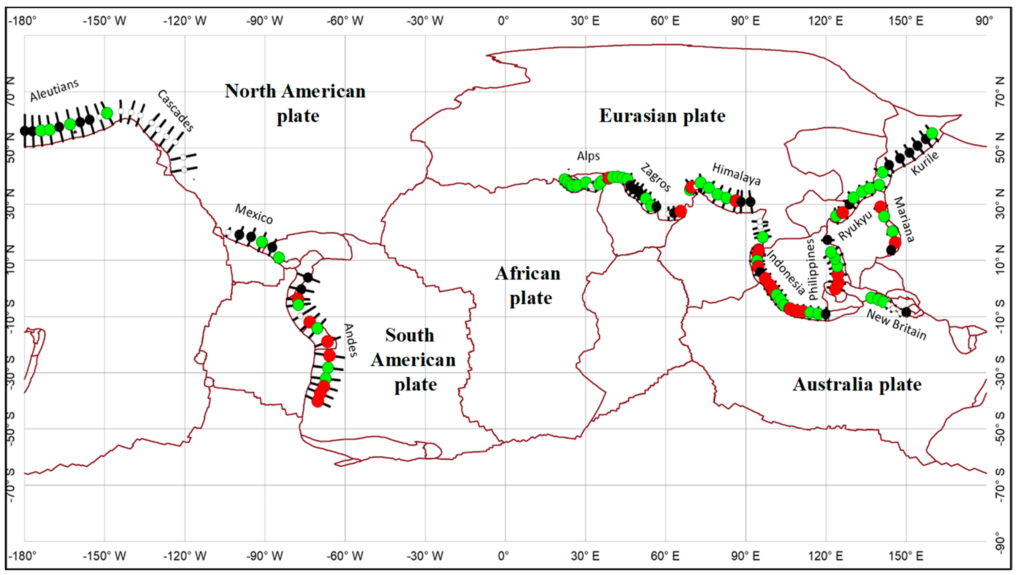
Figure 3. Characteristics of distributions of earthquakes in a buffer area of 100 km around profiles perpendicular to the trench: (A) average depth of earthquakes; (B) number of earthquakes; and (C) the average magnitude of earthquakes. Folded lines represent the boundaries of plates and the short dark blue colored lines for profiles drawn perpendicular to the trench. The dots in the middle of the profile show the average earthquakes with size proportional to average depth, the number of earthquakes, and average magnitudes, respectively.

Figure 3. Characteristics of distributions of earthquakes in a buffer area of 100 km around profiles perpendicular to the trench: (A) average depth of earthquakes; (B) number of earthquakes; and (C) the average magnitude of earthquakes. Folded lines represent the boundaries of plates and the short dark blue colored lines for profiles drawn perpendicular to the trench. The dots in the middle of the profile show the average earthquakes with size proportional to average depth, the number of earthquakes, and average magnitudes, respectively.

5. Results

The basic statistics of earthquakes, including the average depth of earthquakes, the number of earthquakes, and the average magnitudes of earthquakes, in all 130 datasets are given in Table S1 in Supplementary Materials and also shown in Figure 3A–C. The spatial distributions in Figure 3 show that, compared with the Pacific plate’s southeastern boundary, earthquakes on the Pacific plate’s northeastern boundary are generally smaller and shallower. Except for earthquakes near the junctions of plate boundaries, earthquakes on the western Tethys plate converging boundaries are generally smaller and shallower than those on the eastern Tethys plate boundaries. To test whether the earthquakes in each dataset follow the Gutenberg–Richter law, the frequency–magnitudes of earthquakes in several selected sections were calculated and plotted in Figure 4. It was found that some datasets include earthquakes of magnitudes 3 to 7 and others only magnitudes 3–6, without 7. The frequency–magnitudes of the datasets with magnitudes 4–7 can generally be fitted using a GR power law relationship. However, the fittings to datasets with only three magnitudes 4–6 may not have statistical significance.

Instead of frequency–magnitude relationships, the frequency–depth distribution of earthquakes is now explored. For example, the results of the average density of frequency–depth distributions for earthquakes with depths between 34 and 94 km are calculated according to Equation (26a). The results from several selected profiles are shown in Figure 5 (graphs of frequency–depth distributions for the complete list of datasets are given in Supplementary Materials Figures S1–S4). These graphs show profound truncated frequency peaks at 34–44 km. The frequency density decreases rapidly from the peak at 34–44 km downward over 60 km (from 34 to 94 km).

Figure 4. Distribution of frequency–magnitude of earthquakes with magnitudes equal to or greater than 3 from around the Moho with depths ranging from 34 km to 94 km. The GR power law functions (log(N) = a – bM) were fitted to the observed data using least squares. Labels on the graphs indicate the location of the datasets; for example, NA05 and NA07 are datasets 05 and 07 from the North American and Pacific subduction zone; SA indicates the South American and Pacific subduction zone; WP indicates the West Pacific subduction zones; and TB indicates the Tethys Belt.

Figure 4. Distribution of frequency–magnitude of earthquakes with magnitudes equal to or greater than 3 from around the Moho with depths ranging from 34 km to 94 km. The GR power law functions (log(N) = a – bM) were fitted to the observed data using least squares. Labels on the graphs indicate the location of the datasets; for example, NA05 and NA07 are datasets 05 and 07 from the North American and Pacific subduction zone; SA indicates the South American and Pacific subduction zone; WP indicates the West Pacific subduction zones; and TB indicates the Tethys Belt.

Figure 5. Distribution of frequency–depth density of earthquakes with magnitudes equal to or greater than 3 from around the Moho with depths ranging from 34 km to 94 km. The decay curves were calculated with earthquakes with about 5–15% of earthquakes excluded by the threshold of the error of depth <10 km. The frequency density of earthquakes was calculated using Equation (26a). Three types of functions (linear, log-linear, and log–log-linear functions) were fitted to the observed data using least squares. Labels on the graphs indicate the location of the datasets; for example, NA05 and NA07 are datasets 05 and 07 from the North American and Pacific subduction zone; SA indicates the South American and Pacific subduction zone; WP indicates the West Pacific subduction zones; and TB is the Tethys Belt.

Figure 5. Distribution of frequency–depth density of earthquakes with magnitudes equal to or greater than 3 from around the Moho with depths ranging from 34 km to 94 km. The decay curves were calculated with earthquakes with about 5–15% of earthquakes excluded by the threshold of the error of depth <10 km. The frequency density of earthquakes was calculated using Equation (26a). Three types of functions (linear, log-linear, and log–log-linear functions) were fitted to the observed data using least squares. Labels on the graphs indicate the location of the datasets; for example, NA05 and NA07 are datasets 05 and 07 from the North American and Pacific subduction zone; SA indicates the South American and Pacific subduction zone; WP indicates the West Pacific subduction zones; and TB is the Tethys Belt.

Most datasets show a general decay trend in mean earthquake number density as the depth increases from 34 km down to 94 km in 10 km bins. The LS method fitted three types of functions to these data trends. The results of parameters calculated from these LS-fitted functions for all datasets are given in Table S1 in Supplementary Materials. The decay curves in Figure 5 are LS fittings to the data with linear, log-linear (logarithmic), and double log-linear (power law) functions. The likelihoods of fittings are also calculated as coefficients of determination for the LS fittings, and the results are shown in Table S1 in Supplementary Materials. The maximum coefficients of determination were based on determining the function types for the LS fittings. Most of the LS fittings involved in the datasets are statistically significant with R² > 0.9, and the corresponding Student’s t-value > 6.3 (use of 6 points of value for fitting). This means that the datasets can be grouped into three classes according to the types of functions fitted to the data using the LS method. These three decay functions show variable degrees of nonlinearity (linear function, logarithmic function, and power law function) (Figure 6). Before these results are further discussed in the next section, an error assessment should be given to determine how depth errors may affect the results. In addition to the results in Figure 5 that show the decay curves calculated with earthquakes with about 5–15% of earthquakes excluded by the threshold of the error of depth < 10 km, the results are recalculated with all earthquakes from each dataset for comparison. The results for the six datasets used in Figure 5 without filtering of depth errors are given in Supplementary Materials Figure S5, and they indicate that the error filtering of the datasets may slightly affect the values of the estimates of the parameters involved in the LS fittings. Still, it does not change the types of decay functions. Figure S6 in Supplementary Materials shows the distributions of earthquake magnitudes vs. the depth calculated from the datasets as used in Figure 5. The results do not show correlations between magnitudes and depths of earthquakes.

6. Discussion

The spatial distributions of earthquakes classified by the three types of frequency–magnitude relationships (linear, log-linear, and double log-linear) show that the datasets can be roughly divided into two main groups based on their geographic locations separated by 10° N latitudes (Figure 7). The results from earthquakes north of 10° N generally correspond to a linear and log-linear relationship (black and green dots in Figure 7). In contrast, those south of 10° N correspond to a double log-linear relationship (red dots). In addition, linear attenuation relationships are observed from earthquakes in areas such as the Aleutian Islands, Mexico, and the Kuril Islands in the Pacific subduction zone beneath the North American continent. The logarithmic relationships are observed from earthquakes in the mid-low latitude (10° N–40° N) including the areas in Tethys collision zones (Alps, Himalaya) and West Pacific zone (northern Philippines and Ryukyu) underneath Eurasian continents, respectively. Power law relationships are mainly observed from earthquakes in areas in mid-low latitude (10° N–40° S) underneath the South American continents and Eurasian continents, for example, in mid-southeastern Tethys (Indonesia), Southeast Pacific zones (Andes) and Southwest Pacific subduction zones (southern Philippines), respectively. These three types of “linear” relations of the anomalous seismic frequency–depth distribution at depths of 34–44 km downward imply that, from north latitude to south latitude, from the North Pacific subduction zone to the Tethys collision zone, and to the South Pacific subduction zone, the attenuation of the seismic clusters is from linear, to log-linear, to double log-linear.

To further explore the property of the density (ρ), the following differential equation can be used to uniformly represent all three situations with a variable index:

$$\frac{d\rho }{dz}=-c{z}^{-∆\alpha }$$

(27)

The above relationship shows that the rate of density change depends on the depth z from the peak following a power law relation, which gives three special solutions with three values of exponent (Figure 6):

If Δα = 0, then $\frac{d\rho }{dz}=-c,or\rho =-c$z + c₀, where c and c₀ are constant values. This shows that the density decays linearly with the scale of measurement z;

If Δα = 1, then $\frac{d\rho }{dlnz}=-c,or\rho =-clnz+c_0$. This shows that the density scales log-linearly with the scale of measurement;

If Δα ≠ 0, 1, then $\frac{dln(\rho -c_0)}{dlnz}=1-\Delta \alpha ,\ln \left(\rho -c_0\right)=\left(1-\Delta \alpha \right)lnz+\ln \left(\frac{-c}{1-\Delta \mathsf{\alpha }}\right)$. This shows that the density scales double log-linearly with the scale of measurement.

The above three cases show that the nonlinearity of the density of the frequency–depth cluster of earthquakes described with the power law function (27) increases with the value of the power law exponent Δα (=0, 1, and others), from a linear relationship to a log-linear relationship to a double log-linear relationship. Recognizing these differences in decay rate may provide insight into the nonlinearity of the seismic system. Geometrically, the exponent value (Δα) indicates the ratio of the change in density against the change in scale or depth. In the first situation of the linear relationship between density and scale, the factor of c determines the density change rate with the scale change. In the second situation of the log-linear relationship between the density and scale, c determines the ratio of the change rate of the density over the log-transformed scale; and in the third situation of the double log-linear relationship between the density and scale, 1 − ∆α (or α) determines the change rate of log-transformed density over the log-transformed scale.

The above discussions also indicate that the frequency–depth cluster distributions of these three groups of earthquakes can be uniformly described with power law functions, which have different degrees of nonlinearity and are quantified by the index values ∆α (0, 1, and others). In addition to the findings reported in the literature indicating that the distributions of earthquake depths may be related to the physical properties of plates, such as temperature and age, this finding further shows that the attenuation of the peak of shallow seismic frequency–depth distribution around the cluster at about 34–44 km may be related to the aggregation of plates and the continental covers. These results, therefore, provide new insights into the characterization of earthquakes in Tethys and the Pacific converging boundaries. Of course, the specific correlation and mechanism corresponding to these three groups of earthquakes need further investigation, which is out of the scope of the current paper.

Variable frequency–depth distributions of crustal earthquakes and lithological compositions are often integrated to characterize crust deformation about variations in tectonic style [38,39]. For example, a linearly increasing number of earthquakes with depth, followed by a sharp, exponential decrease, has been reported for long, leading to the detection of similar shapes of curves for seismicity distribution and yielding rheological profiles (e.g., [40,41]). Albaric et al. [42] suggested that seismicity peaks and cut-off depths correlate, respectively, with the upper and lower bounds of the brittle–ductile transitions (semi-brittle fields) within the continental crust. The author’s earlier work [6] related the nonlinear distribution of frequency–depth earthquakes to the nonlinear property of rheology in phase transition zones. With the identification of the three linear (linear, log-linear, and double log-linear) decay trends of earthquake frequency–depth cluster at 34–44 km, further study is needed to investigate the impact of these nonlinear patterns with relation to lithosphere rheology around the Moho transition zones.

The mechanical behavior of the Moho as a transition zone with discontinuity of lithosphere separating the crust and the mantle is not only characterized by remarkable changes in seismic wave velocity and lithosphere density but also closely associated with the formation and distribution of earthquakes and other extreme events [43,44,45]. For example, Bird [46] noted that a thrust sheet might readily form through the delamination of the lithosphere at the Moho, as the strength of the upper mantle is far greater than that of the lower crust. Based on field observations of rock deformation, Andersen et al. [44] reported that large Alpine subduction earthquakes might have occurred along the subducting plate’s Moho. A recent study reported a triggering mechanism for earthquakes around the Moho in southern Tibet [47]. There are several factors that Moho transition zones could correspond to the aggregation of earthquakes. These factors include, but are not limited to, changes in density, temperature, pressure, and water fugacity. During the subduction and collision of plates, the solid phase lithosphere can be partially melted to facilitate magma formation and cause strain rate change in the lithosphere, promoting intermediate and deep earthquakes [48]. Both thermal weakening and fluid overpressure weakening can cause active deformation in crustal seismic belts [49,50]. The stress generated by volume change reactions may cause fracturing and potentially trigger earthquakes [50]. It has been substantially studied that an earthquake alters the shear and normal stress on surrounding faults, which causes aftershocks and clusters of earthquakes both spatially and temporally [51]. Phase transition, self-organized criticality, and multiplicative cascade processes are commonly considered to be mechanisms that generate power law distributions of mass or energy density [52]; the power law density differential equation observed from the earthquake data may imply that the Moho as a phase transition zone may be responsible for the clustering of earthquakes around 34–44 km. However, more studies are required to explain what causes the nonlinearity of the clustering distribution of earthquakes around the Moho.

7. Conclusions

According to the properties of the fractal density and the relevant fractal calculus operations defined by the author in this paper based on fractals/multifractals, these concepts can be regarded as extensions of the ordinary physical mass density and calculus defined on regular geometries. Fractal density refers to density defined on fractal geometries with fractal dimensions, so fractal derivatives with fractal dimensions must describe it. In this case, the ordinary density becomes a scale-dependent parameter following a power law relations of scale with two factors, namely fractal density and the exponent or singularity index (∆α), showing the difference between the fractal and the Euclidean dimension. The fractal density reduces to the ordinary density when the fractal dimension becomes the regular Euclidean dimension.

The three types of functions (linear, log-linear, and double log-linear) derived from the fractal density concept fit well the seismic frequency–depth cluster data from all 130 sections perpendicular to plate boundaries within subduction around Pacific plates or in Tethys plates collision zones. These three functions are unified as solutions of a power law differential equation with different exponents 0, 1, or otherwise, characterizing the density decay rate of the seismic frequency–depth cluster. This study attempts to study the frequency–depth cluster distribution of earthquakes from the perspective of fractal density. The nonlinear decay rates represented by these three functions may provide insight into characterizing the clustering of earthquakes in subduction or collision zones.

It should be noted that the precision of the seismic depth data used in this paper varies, so the interpretation of the results should be subject to some degree of uncertainty. More accurate data from earthquakes in the broader area and at other depths should be used in the future to validate the methods and results presented in the current study. One of the questions worthy of further research is the association between the rheological properties of the lithosphere around the Moho and the nonlinearity of the clustering of earthquakes.

References

1. Condie, K.C. Plate Tectonics and Crustal Evolution, 4th ed.; Butterworth-Heinemann: New York, NY, USA, 1997; p. 282. ISBN 978-0-7506-3386-4. [Google Scholar]
2. Schettino, A. Quantitative Plate Tectonics Physics of the Earth—Plate Kinematics—Geodynamics; Springer: New York, NY, USA, 2015; p. 403. [Google Scholar]
3. McKenzie, D.; Jackson, J.; Priestley, K. Thermal structure of oceanic and continental lithosphere. Earth. Planet. Sci. Lett. 2005, 233, 337–349. [Google Scholar] [CrossRef]
4. Cheng, Q. Quantitative simulation and prediction of extreme geological events. Sci. China Earth Sci. 2022, 65, 1012–1029. [Google Scholar] [CrossRef]
5. Atangana, A. Fractional Operators with Constant and Variable Order with Application to Geo-Hydrology; Academic Press: Cambridge, MA, USA, 2018; 390p. [Google Scholar]
6. Patnaik, S.; Hollkamp, J.P.; Semperlotti, F. Applications of variable-order fractional operators: A review. Proc. R. Soc. A. 2020, 476, 498. [Google Scholar] [CrossRef] [PubMed]
7. Li, S.N.; Cao, B.Y. A superstatistical model for anomalous heat conduction and diffusion. Appl. Math. Model. 2020, 79, 392–401. [Google Scholar] [CrossRef]
8. Chen, S.Z.; Liu, F.W.; Turner, I.; Hu, X.L. Numerical inversion of the fractional derivative index and surface thermal flux for an anomalous heat conduction model in a multi-layer medium. Appl. Math. Model. 2018, 59, 514–526. [Google Scholar] [CrossRef]
9. Hristov, J. Steady-state heat conduction in a medium with spatial non-singular fading memory: Derivation of Caputo-Fabrizio space-fractional derivative with Jeffrey’s kernel and analytical solutions. Therm. Sci. 2017, 21, 827–839. [Google Scholar] [CrossRef]
10. Chen, W. Time–space fabric underlying anomalous diffusion. Chaos Solitons Fractals 2006, 28, 923–929. [Google Scholar] [CrossRef]
11. Stewart, J. Fundamental Theorem of Calculus. In Calculus: Early Transcendentals; Thomson/Brooks/Cole: Belmont, CA, USA, 2003; 1308p. [Google Scholar]
12. Scholz, C.H. Earthquakes and friction laws. Nature 1998, 391, 37–42. [Google Scholar] [CrossRef]
13. Song, T.A.; Helmberger, D.V.; Brudzinski, M.R.; Clayton, R.W.; Davis, P.; Pérez-Campos, X.; Singh, S.K. Subducting slab ultra-slow velocity layer coincident with silent earthquakes in southern Mexico. Science 2009, 324, 502–506. [Google Scholar] [CrossRef]
14. Uchida, N.; Kirby, S.H.; Okada, T.; Hino, R.; Hasegawa, A. Supraslab earthquake clusters above the subduction plate boundary offshore Sanriku, northeastern Japan: Seismogenesis in a graveyard of detached seamounts? J. Geophys. Res. 2010, 115, B09308. [Google Scholar] [CrossRef]
15. Varga, P.; Krumm, F.; Riguzzi, F.; Doglioni, C.; Süle, B.; Wang, K.; Panza, G.F. Global pattern of earthquakes and seismic energy distributions: Insights for the mechanisms of plate tectonics. Tectonophysics 2012, 530–531, 80–86. [Google Scholar] [CrossRef]
16. Omori, S.; Komabayashi, T.; Maruyama, S. Dehydration and earthquakes in the subducting slab: Empirical link in intermediate and deep seismic zones. Phys. Earth Planet. Inter. 2004, 146, 297–311. [Google Scholar] [CrossRef]
17. Romanowicz, B. Using seismic waves to image Earth’s internal structure. Nature 2008, 451, 266–268. [Google Scholar] [CrossRef] [PubMed]
18. Kong, X.C.; Li, S.Z.; Suo, Y.H.; Guo, L.L.; Li, X.Y.; Liu, X.; Somerville, I.D.; Dai, L.M.; Zhao, S.J. Hot and cold subduction systems in the Western Pacific Ocean: Insights from heat flows. Geol. J. 2016, 51, 593–608. [Google Scholar] [CrossRef]
19. Okazakl, K.; Hirth, G. Dehydration of lawsonite could directly trigger earthquakes in subducting oceanic crust. Nature 2016, 530, 81–84. [Google Scholar] [CrossRef]
20. Wei, S.S.; Wiens, D.A.; van Keken, P.E.; Cai, C. Slab temperature controls on the Tonga double seismic zone and slab mantle dehydration. Sci. Adv. 2017, 3, e1601755. [Google Scholar] [CrossRef]
21. Gibowicz, S.J. Frequency-magnitude, depth, and time relations for earthquakes in an island arc: North Island, New Zealand. Tectonophysics 1974, 23, 283–297. [Google Scholar] [CrossRef]
22. Cheng, Q.; Sun, H. Variation of singularity of earthquake-size distribution with respect to tectonic regime. Geosci. Front. 2018, 9, 453–458. [Google Scholar] [CrossRef]
23. Hauksson, E.; Meier, M.A. Applying depth distribution of seismicity to determine thermo-mechanical properties of the seismogenic crust in southern California: Comparing lithotectonic blocks. Pure Appl. Geophys. 2019, 176, 1061–1081. [Google Scholar] [CrossRef]
24. McCaffrey, R. Global frequency of magnitude 9 earthquakes. Geology 2008, 36, 263–266. [Google Scholar] [CrossRef]
25. Cheng, Q. Mathematical Geosciences: Local Singularity Analysis of Nonlinear Earth Processes and Extreme Geological Events. In Handbook of Mathematical Geosciences: Fifty Years of IAMG; Daya Sagar, B.S., Cheng, Q., Agterberg, F., Eds.; Springer: Berlin/Heidelberg, Germany, 2018; pp. 179–208. [Google Scholar]
26. Mandelbrot, B.B. The Fractal Geometry of Nature; Freeman Press: New York, NY, USA, 1982; 460p. [Google Scholar]
27. Meakin, P. Fractal aggregates. Adv. Colloid Interface Sci. 1987, 28, 249–331. [Google Scholar] [CrossRef]
28. Schertzer, D.; Lovejoy, S. Physical modeling and analysis of rain and clouds by anisotropic scaling of multiplicative processes. J. Geophys. Res. 1987, 92, 9693–9714. [Google Scholar] [CrossRef]
29. Agterberg, F.P. Mixtures of multiplicative cascade models in geochemistry. Nonlinear Process. Geophys. 2007, 14, 201–209. [Google Scholar] [CrossRef]
30. Lovejoy, S.; Schertzer, D. Scaling and multifractal fields in the solid earth and topography. Nonlinear Process. Geophys. 2007, 14, 465–502. [Google Scholar] [CrossRef]
31. Malamud, B.D.; Turcotte, D.L.; Barton, C.C. The 1993 Mississippi river flood: A one hundred or a one thousand year event? Environ. Eng. Geosci. 1996, 2, 479–486. [Google Scholar] [CrossRef]
32. Turcotte, D.L. Fractals and Chaos in Geology and Geophysics, 2nd ed.; Cambridge University Press: Cambridge, UK, 1997; 398p. [Google Scholar]
33. Veneziano, D. Multifractality of rainfall and scaling of intensityduration-frequency curves. Water Resour. Res. 2002, 38, 42-1–42-12. [Google Scholar] [CrossRef]
34. Agterberg, F.P. Multifractal modeling of the sizes and grades of giant and supergiant deposits. Int. Geol. Rev. 1995, 37, 1–8. [Google Scholar] [CrossRef]
35. Agterberg, F.P. Multifractal simulation of geochemical map patterns. In Geologic Modeling and Simulation: Sedimentary Systems; Merriam, D.F., Davis, J.C., Eds.; Kluwer: New York, NY, USA, 2001; pp. 327–346. [Google Scholar]
36. Cheng, Q. Generalized binomial multiplicative cascade processes and asymmetrical multifractal distributions. Nonlinear Process. Geophys. 2014, 21, 477–487. [Google Scholar] [CrossRef]
37. Rogers, N.; Blake, S.; Burton, K. An Introduction to Our Dynamic Planet; Cambridge University Press: Cambridge, UK, 2008; p. 19. ISBN 978-0-521-49424-3. [Google Scholar]
38. Déverchère, J.; Petit, C.; Gileva, N.; Radziminovitch, N.; Melnikova, V.; San’kov, V. Depth distribution of earthquakes in the Baikal rift system and its implications for the rheology of the lithosphere. Geophys. J. Int. 2001, 146, 714–730. [Google Scholar] [CrossRef]
39. Mouthereau, F.; Petit, C. Rheology and strength of the Eurasian continental lithosphere in the foreland of the Taiwan collision belt: Constraints from seismicity, flexure, and structural styles. J. Geophys. Res. 2003, 108, 2512. [Google Scholar] [CrossRef]
40. Fadaie, K.; Ranalli, G. Rheology of the lithosphere in the East African Rift System. Geophys. J. Int. 1990, 102, 445–453. [Google Scholar] [CrossRef]
41. Lamontagne, M.; Ranalli, G. Thermal and rheological constraints on the earthquake depth distribution in the Charlevoix, Canada, intraplate seismic zone. Tectonophysics 1996, 257, 55–69. [Google Scholar] [CrossRef]
42. Albaric, J.; Déverchère, J.; Petit, C.; Perrot, J.; Le Gall, B. Crustal rheology and depth distribution of earthquakes: Insights from the central and southern East African Rift System. Tectonophysics 2009, 468, 28–41. [Google Scholar] [CrossRef]
43. Chen, W.; Yang, Z. Earthquakes beneath the Himalayas and Tibet: Evidence for strong lithospheric mantle. Science 2004, 304, 1949–1951. [Google Scholar] [CrossRef]
44. Andersen, T.B.; Austrheim, H.; Deseta, N.; Silkoset, P.; Ashwal, L.D. Large subduction earthquakes along the fossil Moho in Alpine Corsica. Geology 2014, 42, 395–398. [Google Scholar] [CrossRef]
45. Goswami, A.; Barbot, S. Slow-slip events in semi-brittle serpentinite fault zones. Sci. Rep. 2018, 8, 6181. [Google Scholar] [CrossRef] [PubMed]
46. Bird, P. Initiation of intracontinental subduction in the Himalaya. J. Geophys. Res. 1978, 83, 4975–4987. [Google Scholar] [CrossRef]
47. Shi, F.; Wang, Y.; Yu, T.; Zhu, L.; Zhang, J.; Wen, J.; Gasc, J.; Incel, S.; Schubnel, A.; Li, Z.; et al. Lower-crustal earthquakes in southern Tibet are linked to eclogitization of dry metastable granulite. Nat. Commun. 2018, 9, 3483. [Google Scholar] [CrossRef]
48. Dimanov, A.; Wirth, R.; Dresen, G. The effect of melt distribution on the rheology of plagioclase rocks. Tectonophysics 2000, 328, 307–327. [Google Scholar] [CrossRef]
49. Sibson, R.H.; Rowland, J.V. Stress, fluid pressure and structural permeability in seismogenic crust, North Island, New Zealand. Geophys. J. Int. 2003, 154, 584–594. [Google Scholar] [CrossRef]
50. Pontbriand, C.W.; Sohn, R.A. Microearthquake evidence for reaction-driven cracking within the Trans-Atlantic geotraverse active hydrothermal deposit. J. Geophys. Res. 2014, 119, 822–839. [Google Scholar] [CrossRef]
51. Stein, R.S. The role of stress transfer in earthquake occurrence. Nature 1999, 402, 605–609. [Google Scholar] [CrossRef]
52. Bak, P.; Tang, C.; Wiesenfeld, K. Self-organized criticality: An explanation of 1/f noise. Phys. Rev. Lett. 1987, 59, 381–384. [Google Scholar] [CrossRef] [PubMed]
Figure 1. Processes forming binomial multifractals distribution. The iteration starts as unit length L (unit of meter) and unit height m (e.g., m stands for the total metal mass in a unit of g). In each iteration, the parent length is further divided into three equal segments (εn = 1/3εn−1), and one segment receives more proportion of the metal redistributed from the middle segment than the other segments. So the metal in the middle segment equals zero, while those in the two remaining segments receive d · m and (1 − d) · m (0 < d < 1), respectively. The coefficient of dispersion (d) is independent of segment size.
Fractalfract 07 00721 g001
Figure 2. Study areas were chosen along the Tethys and Pacific converging plate boundaries: (A) Distribution of earthquakes of magnitudes 7 and above from the International Seismic Data Center (ISC). The background color image represents the digital elevation model (ETOPO1). (B) Schematic diagram showing the seismogenic zone in the context of plate tectonics. The red box indicates the selected region 300 km from the trench from where the earthquake data were extracted. Red stars stand for earthquakes. Dashed blue line indicates Moho of oceanic lithosphere. (C) Profile showing the distribution of earthquakes at the long section perpendicular to the trench. Three sections 100 km apart from South America along the subduction zone of the Pacific Ring. The green oval shapes indicate those few earthquakes located apart from the cluster of earthquakes sketching the shape of slabs were excluded from the analysis due to a potential problem either by inaccurate depth or different types of earthquakes. Data containing earthquakes with magnitudes M ≥ 3 and their depths were downloaded from the USGS website.
Fractalfract 07 00721 g002
Figure 6. Illustrative diagram showing the relationship between density r and depth z. Three lines show solutions from the differential equation as shown in the figure with three exponent values: ∆α= 0 or 1, and otherwise.
Fractalfract 07 00721 g006
Figure 7. Locations of three types of relations between the frequency and depth of earthquakes from Pacific and Tethys converging boundaries. The relations show the data fitted using a linear function (black dots), a log-linear function (green dots), and a log–log-linear function (red dots). Log-linear function (logarithmic function) (green dots) and double log-linear function (power law function) are also shown. Small circles represent the dataset without functions fitting either due to the insufficient number of earthquakes or no profound trend of distribution. Folded line segments represent the boundaries of tectonic plates.
Fractalfract 07 00721 g007
Disclaimer/Publisher’s Note: The statements, opinions and data contained in all publications are solely those of the individual author(s) and contributor(s) and not of MDPI and/or the editor(s). MDPI and/or the editor(s) disclaim responsibility for any injury to people or property resulting from any ideas, methods, instructions or products referred to in the content.