
Non-Linear Analysis of Novel Equivalent Circuits of Single-Diode Solar Cell Models with Voltage-Dependent Resistance
 , , ,
, , ,  ,
,  and
and 
(This article belongs to the Section Engineering)
Abstract
:1. Introduction
1.1. Background
1.2. Motivation
1.3. Methodology
1.4. Novelty and Contributions
- Three new variants of the single-diode model of solar cells are proposed.
- The voltage dependence of the series resistance, parallel resistance and both of them are considered.
- Analytical expressions for current-voltage dependences of the proposed solar cell models are derived using the Lambert W function.
- An improved snake optimization algorithm using chaotic sequences is presented in this work for estimating the parameters of the investigated solar cell and module.
- The results of comparing the proposed algorithm and numerous literature-known algorithms are presented.
- An experimental investigation was conducted into the applicability of the proposed models to a solar laboratory module, and the results obtained proved the relevance and effectiveness of the proposed models.
1.5. Organization
2. Single-Diode Solar Cell Model and Discussion of the Related Literature
2.1. Basic Information about the Standard Single-Diode Solar Cell Model
2.2. Discussion of the Related Literature Review
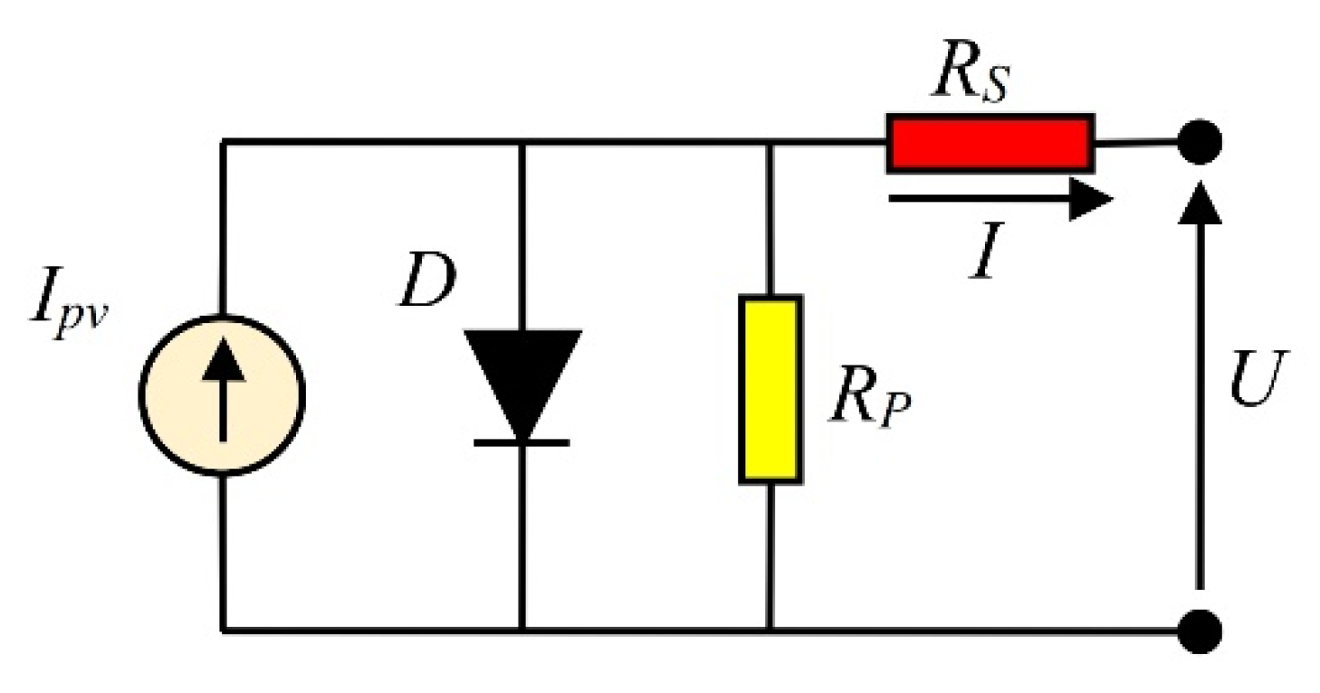
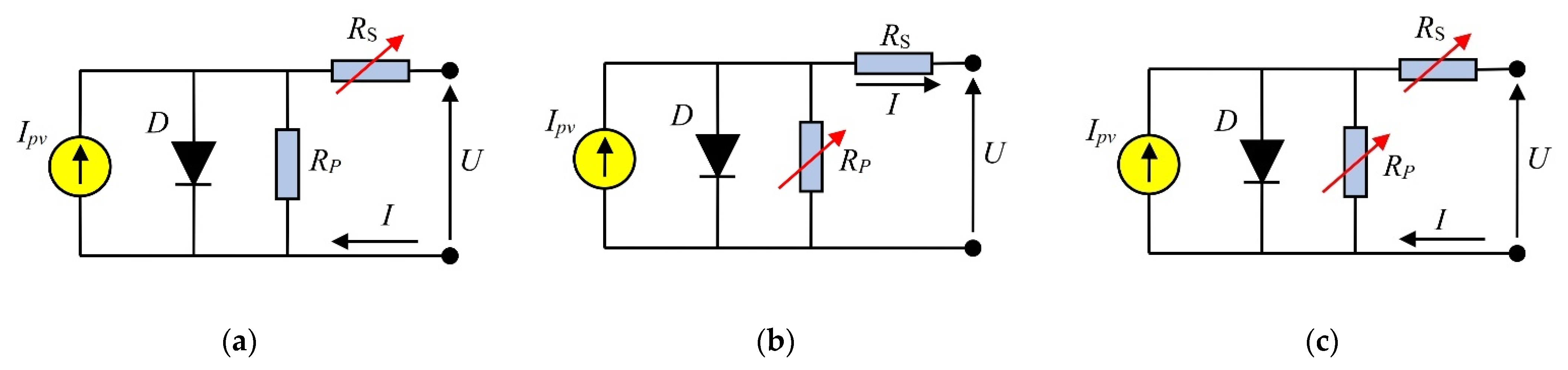
3. Equivalent Circuits Proposed
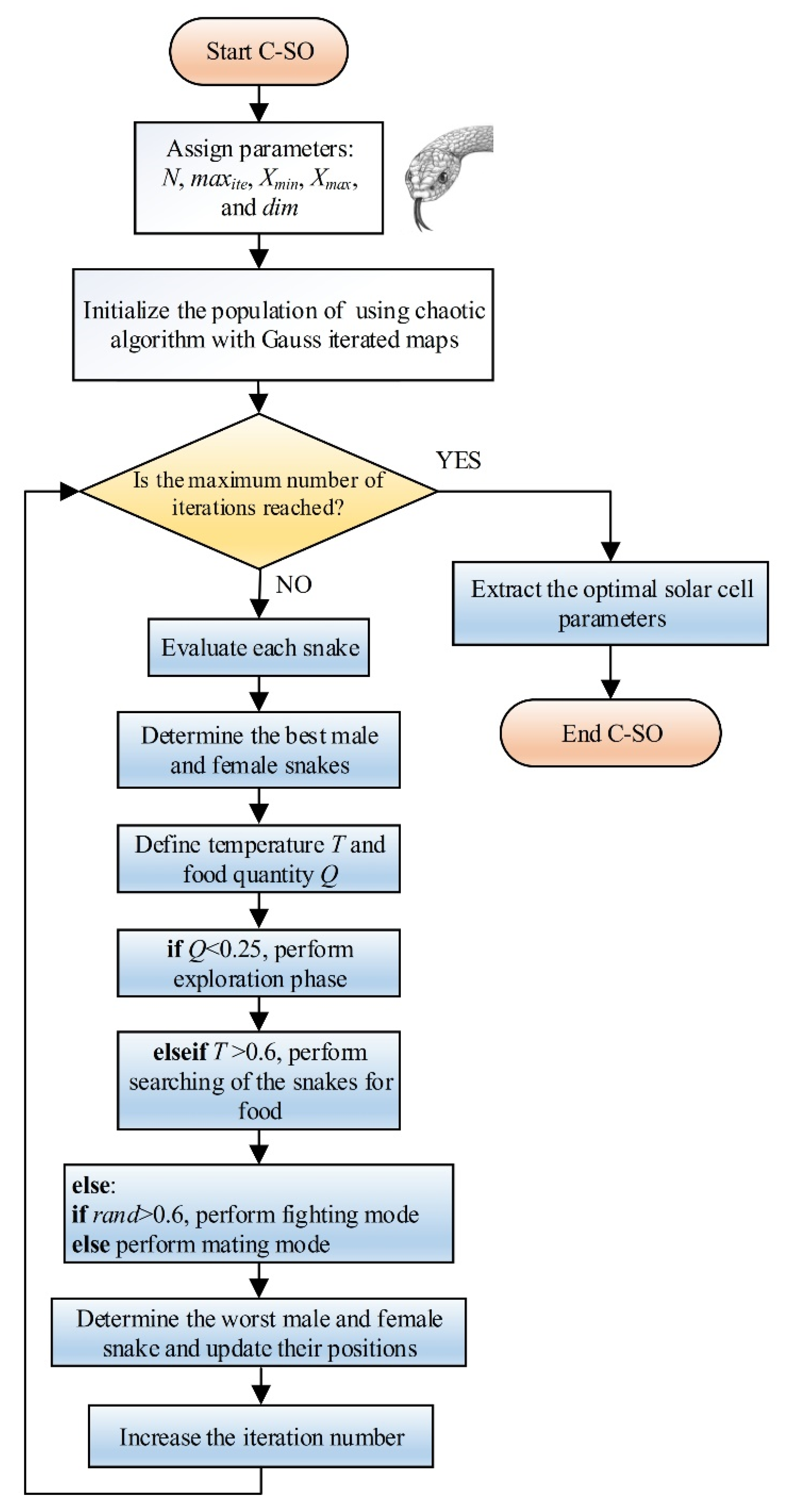
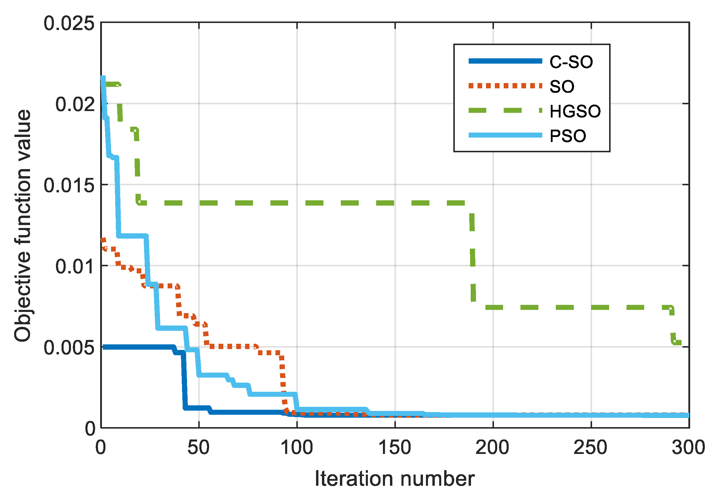
4. Chaotic SO Algorithm Proposed
| Algorithm 1 Procedure of the Proposed C-SO Algorithm |
|
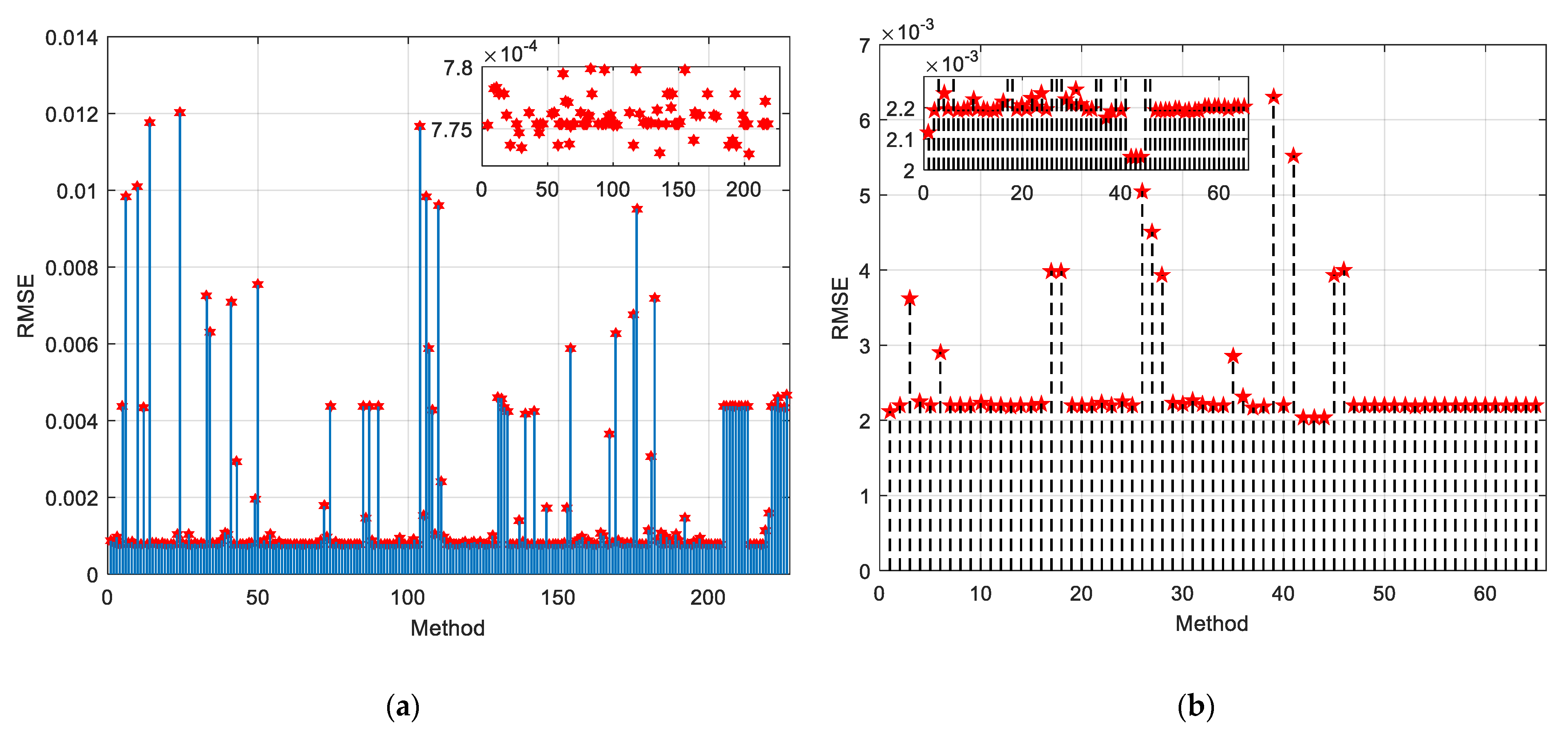
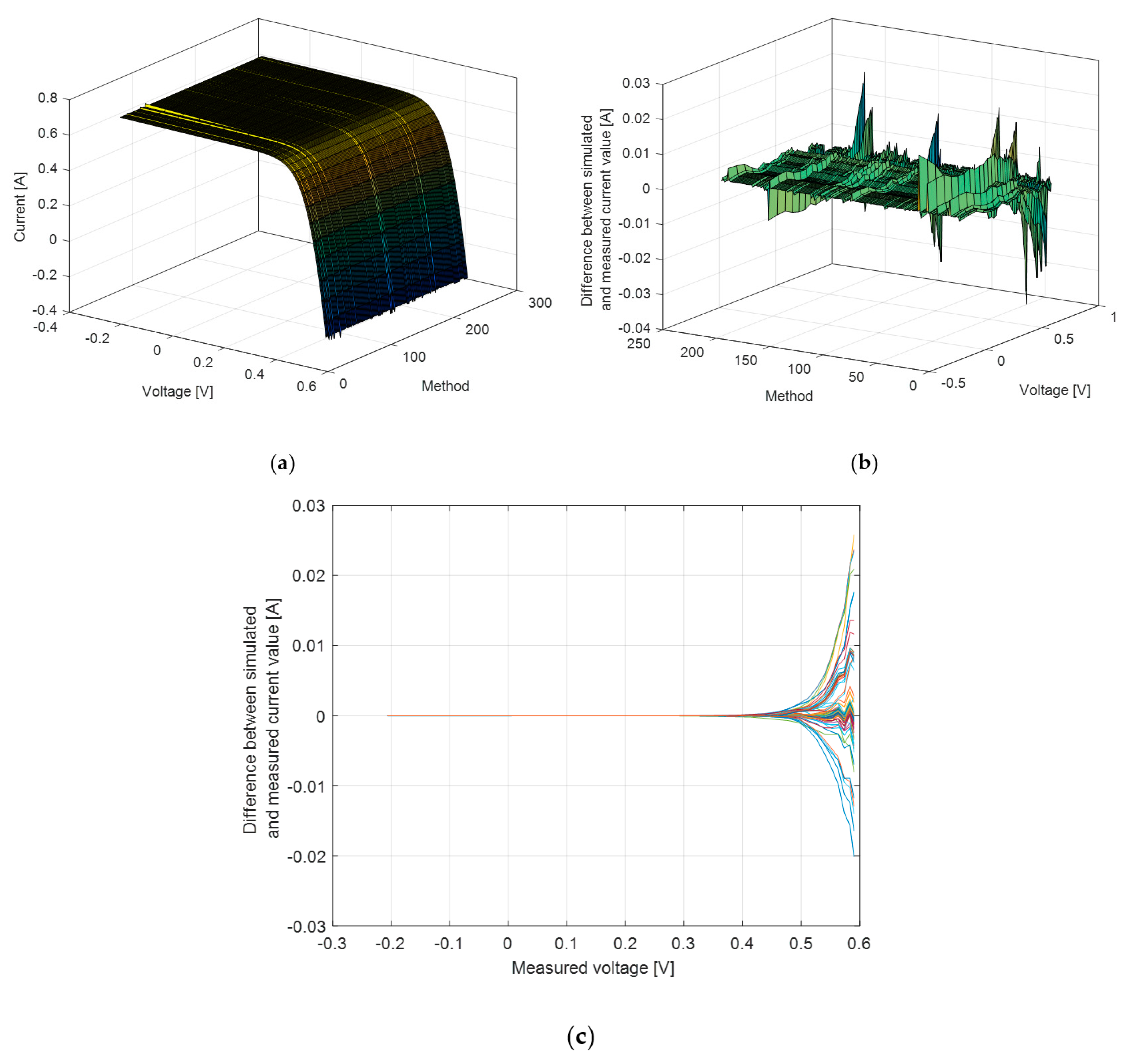
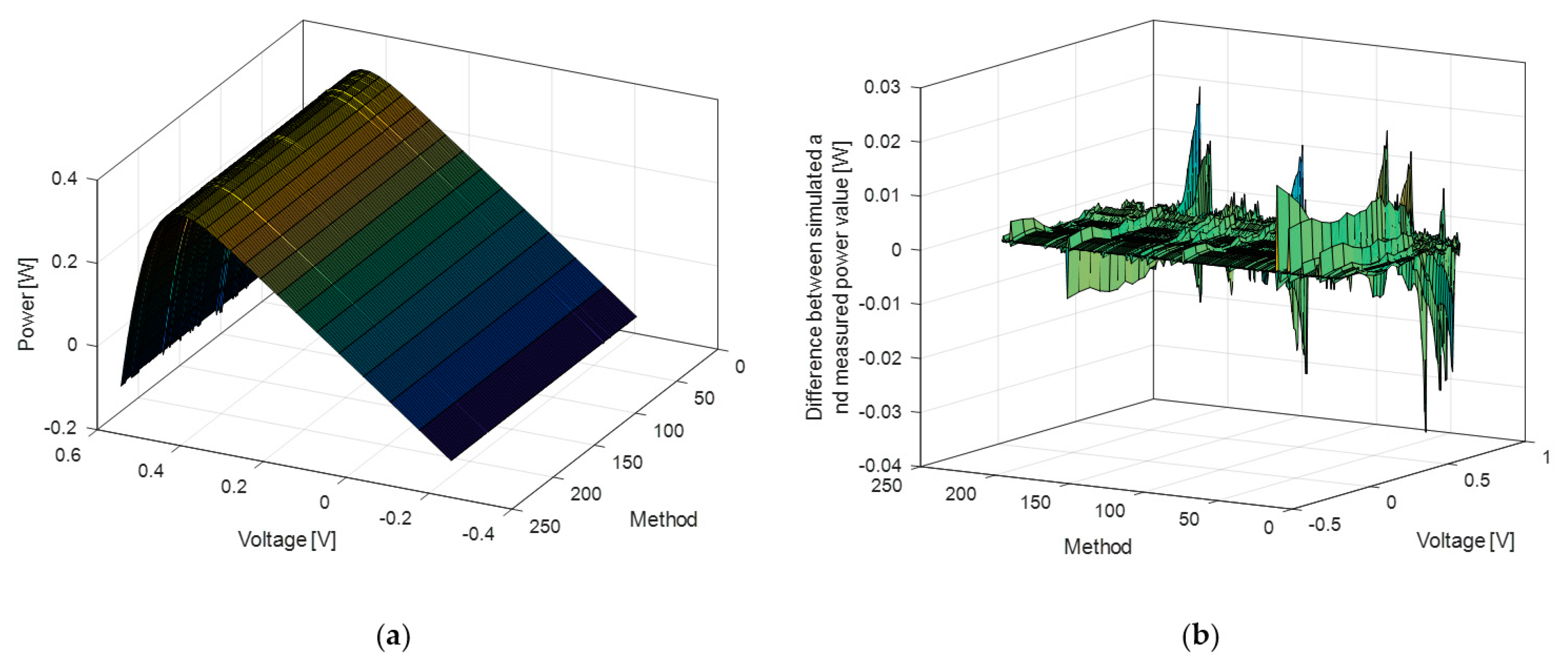
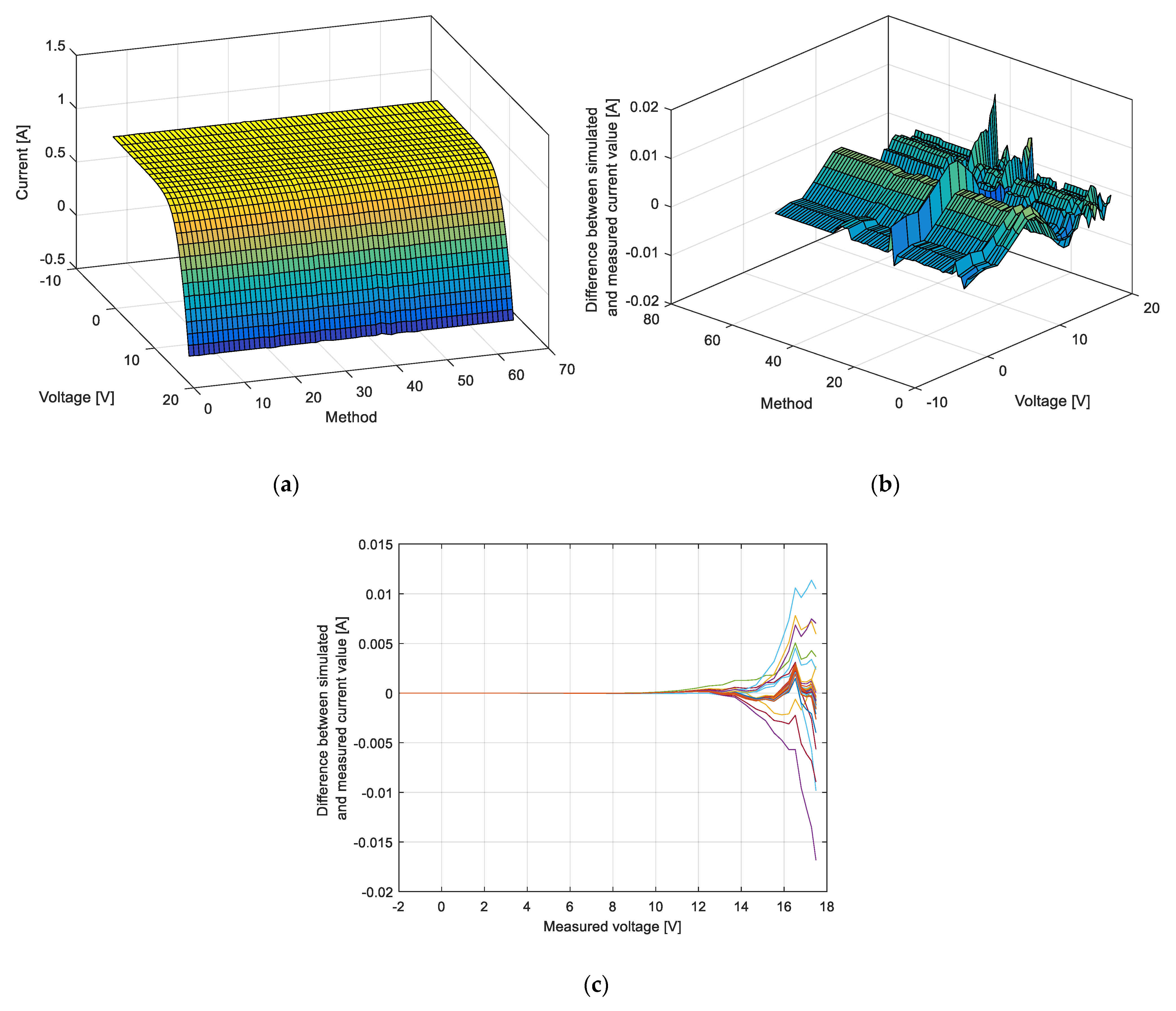
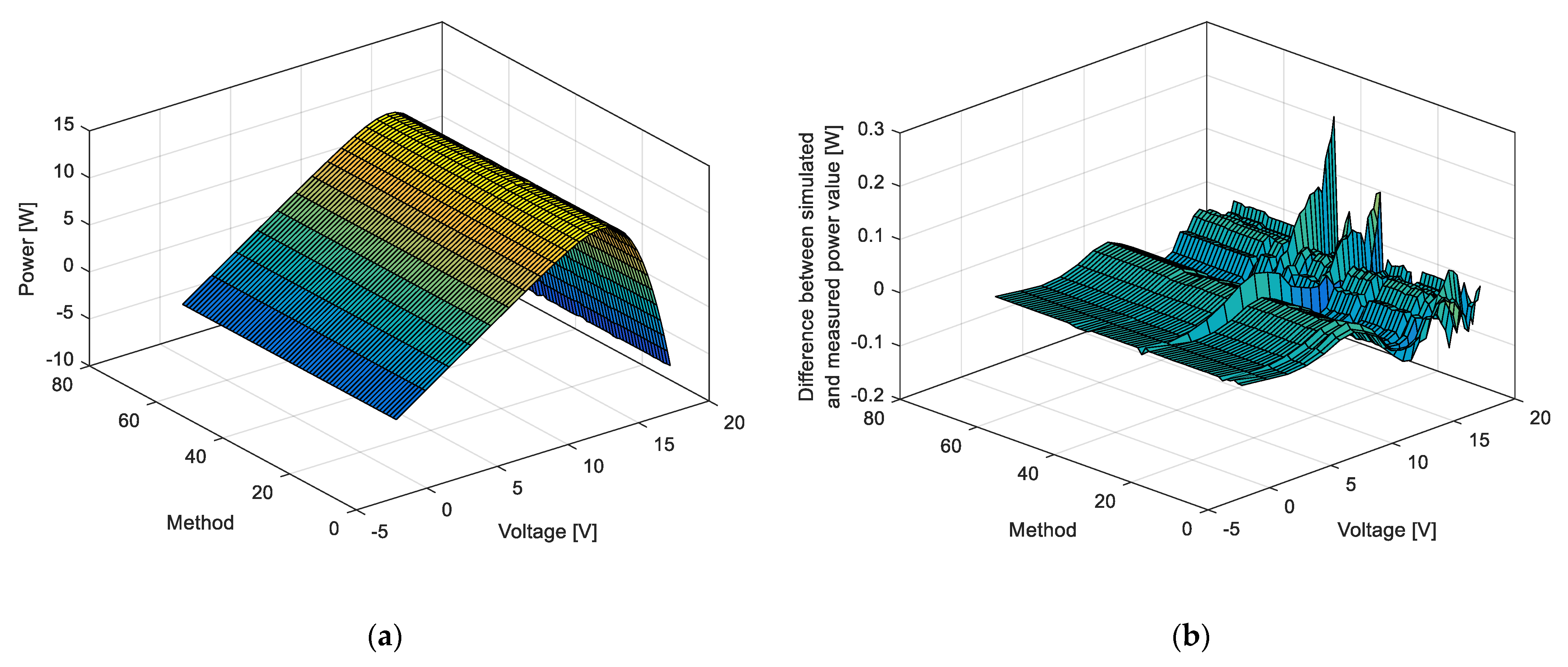
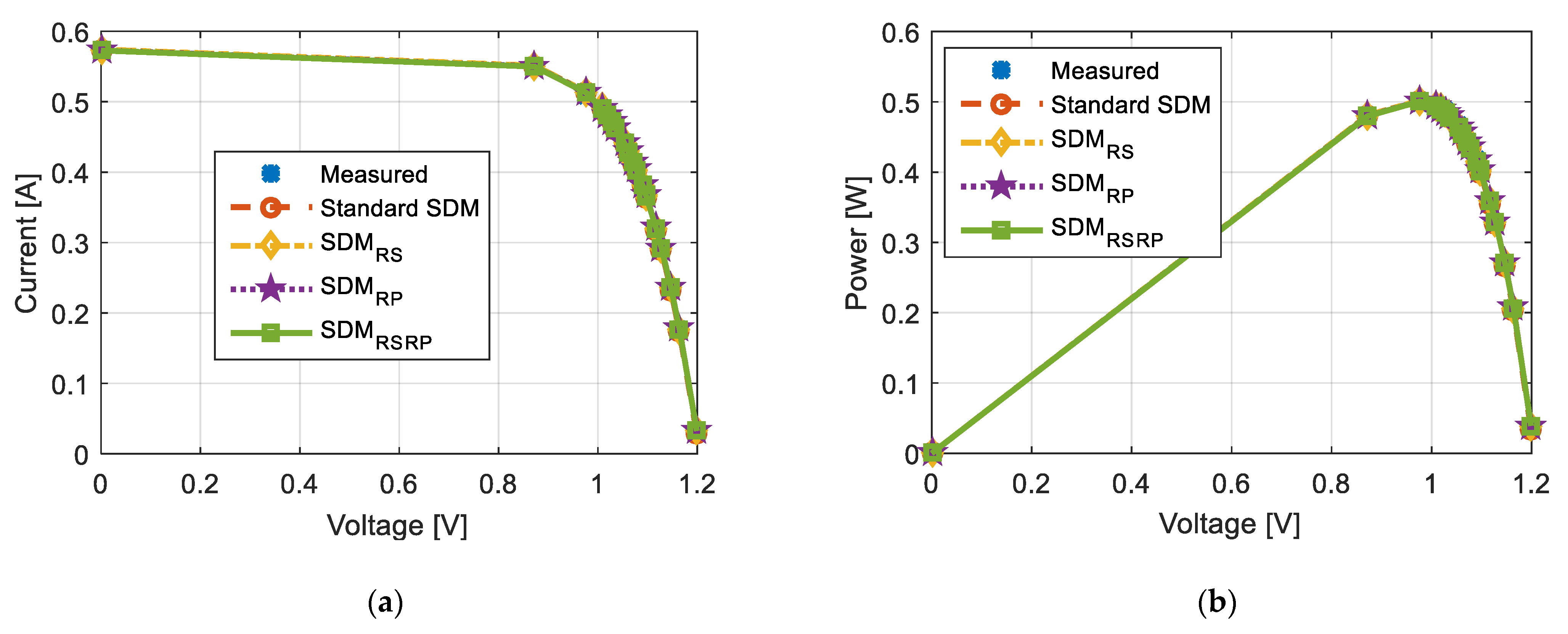
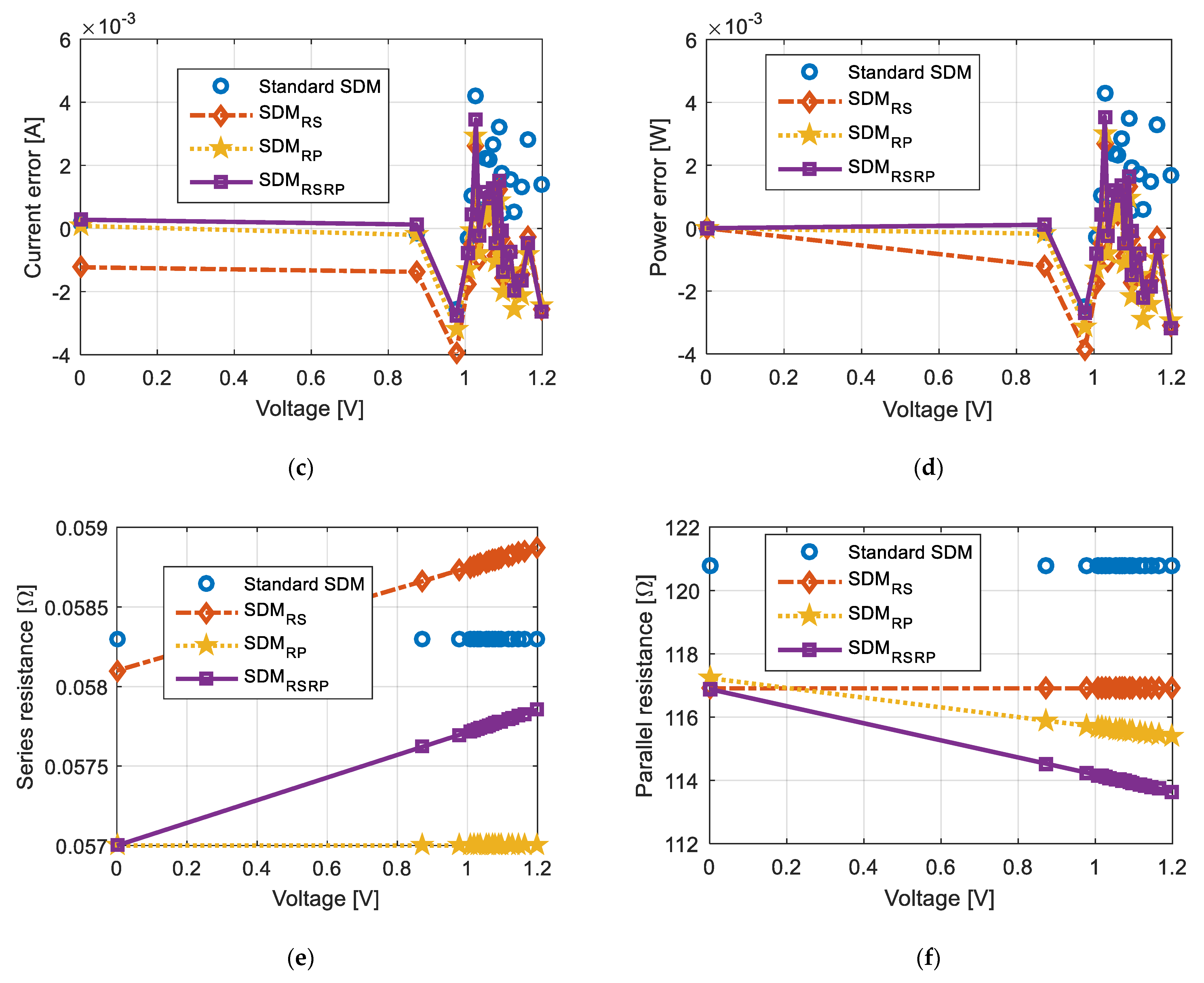
5. Numerical Results
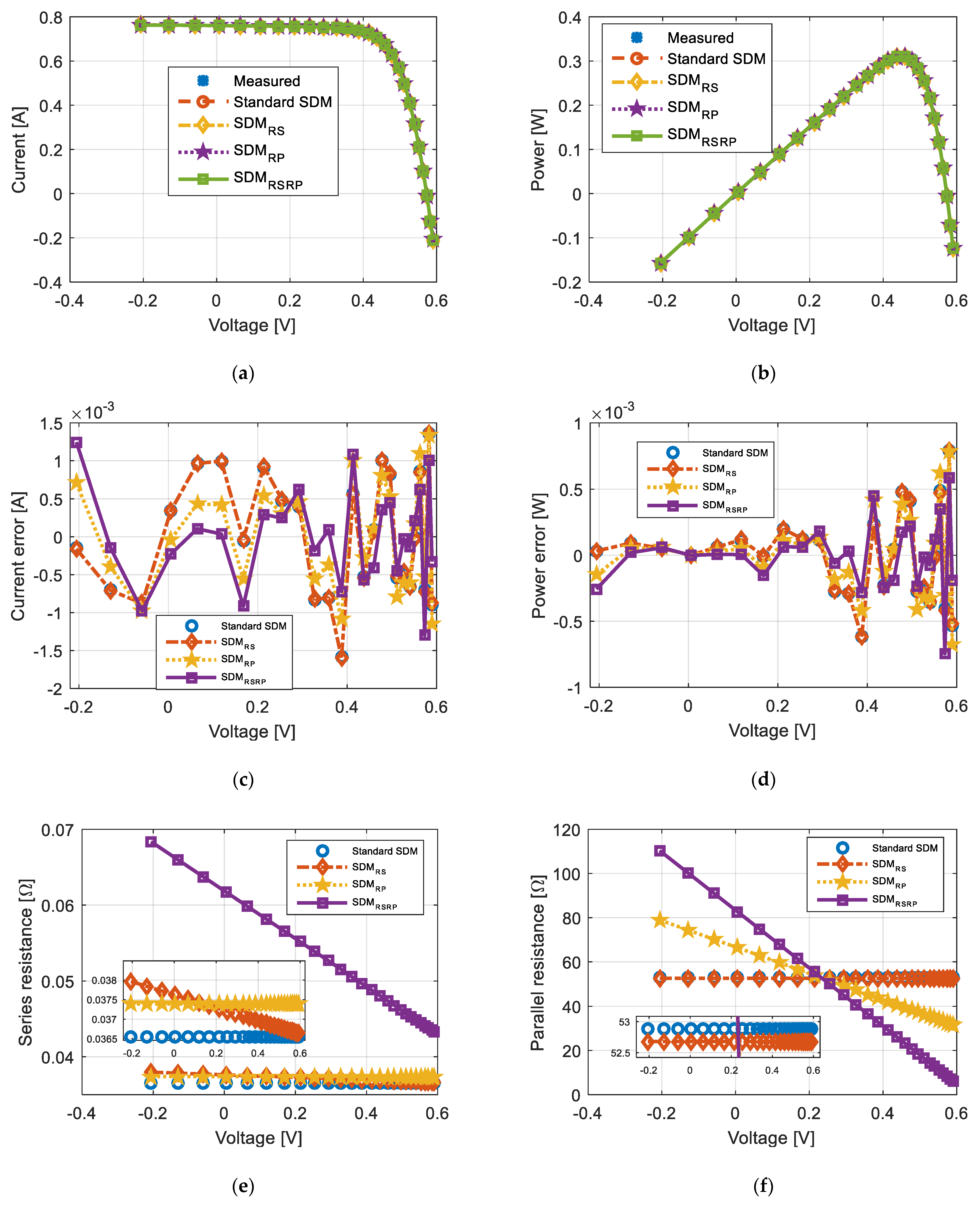
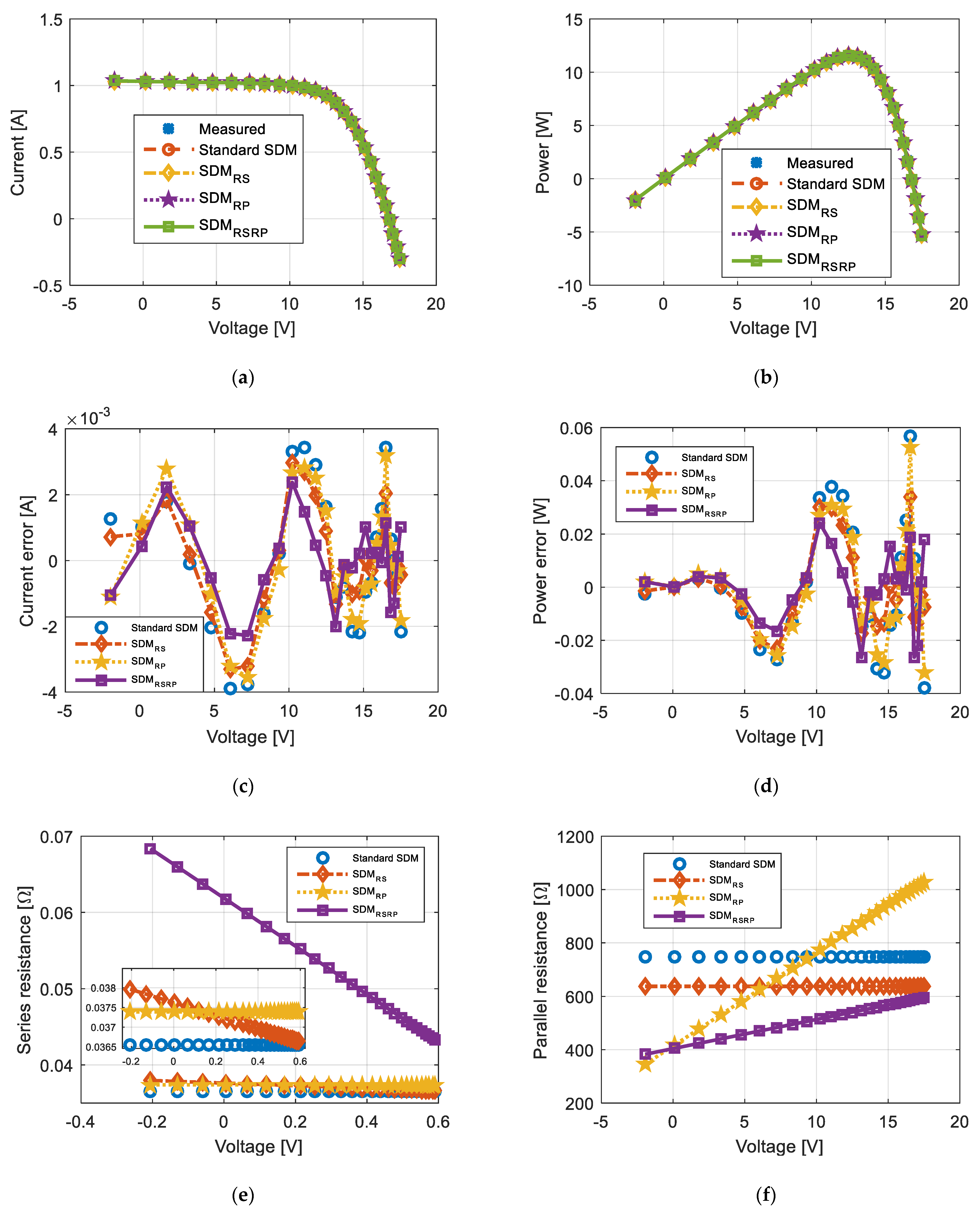
- Recalling Section 2, the RMSE for RTC France solar cell determined for standard SDM is 7.730062689943169 × 10⁻⁴, slightly better than the results available in the literature. For the Photowatt-PWP201 module, the RMSE is 0.002039992273216, which is a better result than the results available in the literature.
- Additionally, the voltage dependence of RP or RS or both enables better fitting between the measured and simulated characteristics for both investigated solar cells/modules.
- The impact of voltage dependence on individual series or parallel resistance cannot be generally guaranteed as a better effect of the voltage dependence of series resistance for the Photowatt-PWP201 module on the results was observed in Table 2. In contrast, a better impact of the voltage dependence of the parallel resistance for the RTC France solar cell was observed in Table 1.
- The value of RMSE can be reduced by 40% for the Photowatt-PWP201 module and 20% for RTC France solar cell, considering the voltage dependence of both resistances in the solar cell model. Therefore, the matching between measured and simulated curves is significantly improved.
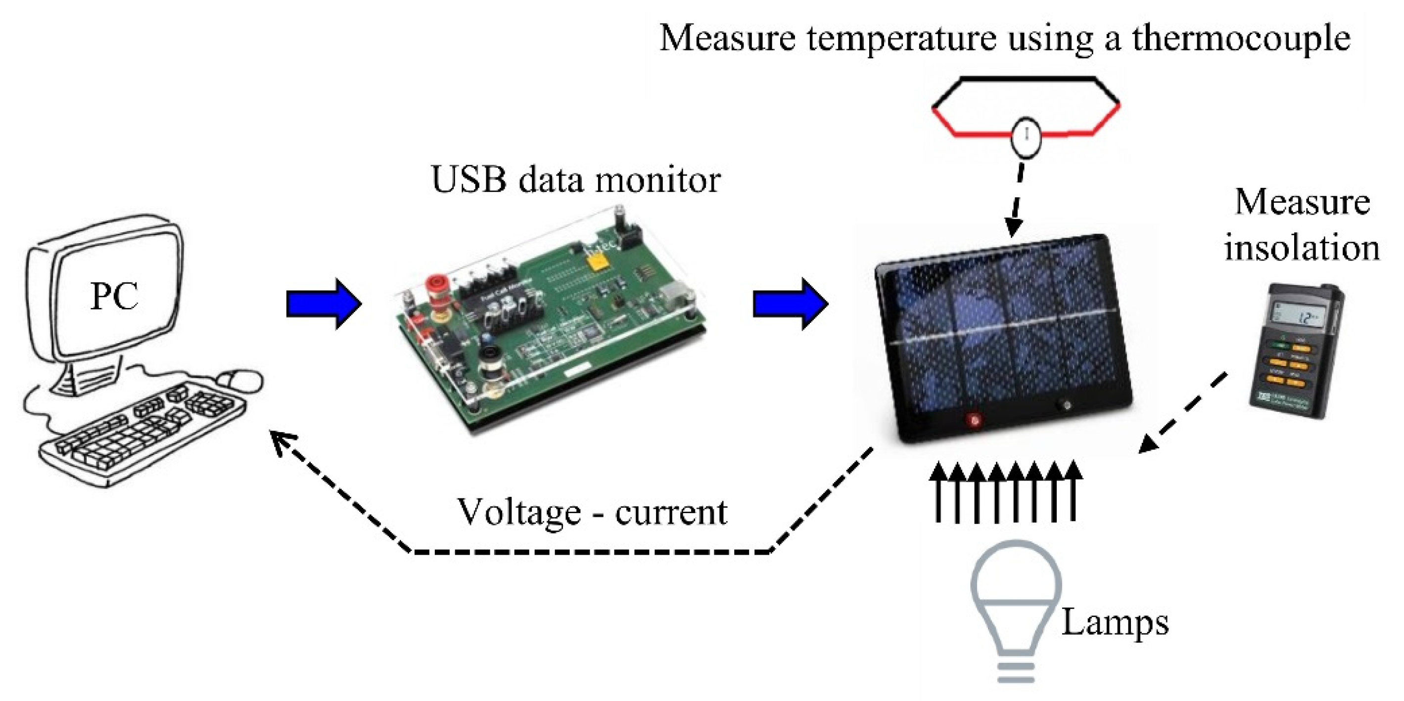
6. Experimental Verification
7. Conclusions
Author Contributions
Funding
Data Availability Statement
Acknowledgments
Conflicts of Interest
Abbreviations
| ABC | Artificial bee colony |
| ABCTRR | Trust-region reflective (TRR) deterministic algorithm with the artificial bee colony (ABC) metaheuristic algorithm |
| ABSO | General algorithm for finding the absolute minimum of a function to a given accuracy |
| AGDE | Adaptive guided differential evolution |
| ALO | Ant Lion optimization algorithm |
| BBO | Biogeography-based optimization |
| BPFPA | Bee pollinator flower pollination algorithm |
| BLPSO | Biogeography-based learning particle swarm optimization |
| BLPSO | Biogeography-based learning PSO |
| BHCS | Hybridizes cuckoo search (CS) and biogeography-based |
| BMO | Bird mating optimization |
| BSA | Backtracking search algorithm |
| CPSO | Chaos particle swarm optimization |
| CS | Cuckoo search |
| CSO | Competitive swarm optimizer |
| CSA | Competitive swarm algorithm |
| CMM-DE/BBO | DE/BBO with covariance matrix-based migration |
| CLPSO | Comprehensive learning particle swarm optimization |
| CIABC | Chaotic improved the artificial bee colony |
| CNSMA | Boosting slime mould algorithm |
| COA | Chaotic optimization approach |
| COOA | Coyote optimization algorithm |
| CWOA | Chaotic whale optimization algorithm |
| CPSO | Conventional PSO |
| CPMPSO | Classified perturbation mutation-based PSO |
| DGM | Dynamic gaussian mutation |
| DE | Differential evolution |
| DE/BBO | Hybrid differential evolution with biogeography-based optimization |
| DE/WOA | Differential evolution/whale optimization algorithm |
| EHHO | Enhanced Harris Hawks optimization |
| ERWCA | Evaporation rate water cycle algorithm |
| EDDM-LW | Explicit double-diode model based on the Lambert W function |
| EO | Equilibrium optimizer |
| EOTLBO | Equilibrium optimizer teaching-learning-based optimization |
| EJADE | Enhanced joint approximation diagonalization of Eigen matrices algorithm |
| ELPSO | Enhanced leader particle swarm optimization |
| ELBA | Efficient layer-based routing algorithm |
| EGBO | Enhanced gradient-based optimization |
| EVPS | Enhanced vibrating particles systems |
| FA | Firefly algorithm |
| FCEPSO | Fractional chaotic ensemble particle swarm optimizer |
| FPA | Flower pollination algorithm |
| FPSO | Fuzzy particle swarm optimization |
| HCLPSO | Chaotic heterogeneous comprehensive learning particle swarm optimizer variants |
| HPSOSA | Hybrid particle swarm optimization and simulated annealing |
| HFAPS | Hybrid firefly and pattern search algorithms |
| HISA | Hyperplanes intersection simulated annealing |
| HS | Harmony search |
| HSMAWOA | Hybrid novel slime mould algorithm with a whale optimization algorithm |
| GA | Genetic algorithm |
| GABC | Gbest guided ABC |
| GAMNU | Genetic algorithm based on non-uniform mutation |
| GAMS | General algebraic modeling system |
| GCPSO | Guaranteed convergence particle swarm optimization |
| GGHS | Gaussian global-best harmony search |
| GSK | Gaining-sharing knowledge-based algorithm |
| GOTLBO | Generalized oppositional teaching learning-based optimization |
| GOFPNAM | Algorithm based on FPA, the Nelder-Mead simplex, and the GOBL mechanism |
| GBABC | Gaussian bare-bones ABC |
| GWO | Grey wolf optimizer |
| GWOCS | Grey wolf optimizer cuckoo search |
| HS | Harmony search |
| HHO | Harris Hawks optimization |
| HCLPSO | Heterogeneous comprehensive learning particle swarm optimizer |
| ICA | Independent component analysis |
| ISCA | Improved sine cosine algorithm |
| ISCE | Improved shuffled complex evolution |
| ISMA | Index-based subgraph matching algorithm |
| IADE | Improved differential evolution algorithm |
| IBBGOA | Interval branch and bound global optimization algorithm |
| IJAYA | Improved JAYA |
| IGHS | Improved Gaussian harmony search |
| IMFO | Improved moth-flame optimization |
| ITLBO | Improved teaching-learning-based optimization |
| IWOA | Improved whale optimization algorithm |
| JADE | Joint approximation diagonalization of Eigen matrices algorithm |
| jDE | Self-adaptive DE algorithm |
| LAPO | Lightning attachment procedure optimization |
| LCJAYA | Logistic chaotic JAYA algorithm |
| LETLBO | TLBO with a learning experience of other learners |
| LBSA | List-based simulated annealing algorithm |
| LSP | Loop of the search process |
| LMSA | Least mean squares (LMS) algorithms |
| MADE | Memetic adaptive differential evolution |
| MABC | Modified ABC |
| MJA | Modified JAYA algorithm |
| MLBSA | Modified list-based simulated annealing algorithm |
| MPA | Marine predator algorithm |
| MFO | Moth-flame Optimization |
| MPSO | Particle swarm optimization with adaptive mutation strategy |
| MPCOA | Mutative-scale parallel chaos optimization algorithm |
| MRFO | Manta ray foraging optimization |
| MSSO | Modified simplified swarm optimization |
| MVO | Multi-verse optimizer |
| nm-NMPSO | Nelder-Mead and modified particle swarm optimization |
| NMMFO | Nelder–Mead moth flame method |
| NIWTLBO | Non-linear inertia weighted TLBO |
| NRM | Newton Raphson method |
| NPSOPC | Niche particle swarm optimization in parallel computing |
| ODE | Opposition-based differential evolution |
| PGJAYA | Performance-guided JAYA |
| pSFS | Perturbed stochastic fractal search |
| PS | Pattern search |
| PSO | Particle swarm algorithm |
| PPSO | Parallel particle swarm optimization |
| RLDE | Run length encoding (RLE) compression algorithm |
| RTLBO | Ranking teaching-learning-based optimization |
| R-II | Rao-2 algorithm |
| R-III | Rao-3 algorithm |
| SA | Simulated annealing |
| SaDE | Self-adaptive differential evolution algorithm |
| SDA | Successive discretization algorithm |
| SDE | Stochastic differential evolution |
| SGDE | Stochastic gradient descent algorithm |
| SHADE | Success-history-based parameter adaptation for differential evolution |
| SCA | Sine cosine algorithm |
| SATLBO | Self-adaptive teaching-learning-based optimization |
| SMA | Slime mould algorithm |
| SFS | Stochastic fractal search |
| STLBO | Simplified TLBO |
| SATLBO | Simulated annealing TLBO |
| SOS | Symbiotic organisms search |
| SSA | Salp swarm algorithm |
| SSO | Simplified swarm optimization |
| TLABC | Teaching-learning-based artificial bee colony |
| TLBO | Teaching-learning-based optimization |
| TLO | Teaching-learning optimization |
| TVACPSO | Time-varying acceleration coefficients particle swarm optimization |
| TVAPSO | Time-varying particle swarm optimization |
| WLCSODGM | Winner-leading CSO with DGM |
| WCMFO | Hybrid algorithm based on the water cycle and moth-flame optimization algorithm |
| WOA | Whale optimization algorithm |
| WDO | Wind-driven optimization |
| WHHO | Whippy harris hawks optimization |
Appendix A

| Method | Reference | Algorithm | Ipv (A) | I0 (μA) | n | RS (Ω) | RP (Ω) |
|---|---|---|---|---|---|---|---|
| 1 | [15] | EO | 0.760759704 | 0.32628893 | 1.482193 | 0.036341 | 54.206594 |
| 2 | MPA | 0.76079 | 0.31072 | 1.4771 | 0.036546 | 52.8871 | |
| 3 | HCLPSO | 0.76079 | 0.31062 | 1.4771 | 0.036548 | 52.885 | |
| 4 | BPFPA | 0.76 | 0.3106 | 1.4774 | 0.0366 | 57.7151 | |
| 5 | ER-WCA | 0.760776 | 0.322699 | 1.48108 | 0.036381 | 53.691 | |
| 6 | MPSO | 0.760787 | 0.310683 | 1.475262 | 0.036546 | 52.88971 | |
| 7 | PS | 0.7617 | 0.998 | 1.6 | 0.0313 | 64.10236 | |
| 8 | [25] | BBO-M | 0.7607 | 3.19 × 10⁻¹ | 1.4798 | 0.03642 | 53.36227 |
| 9 | IMFO | 0.7607 | 3.23 × 10⁻¹ | 1.4812 | 0.03638 | 53.71456 | |
| 10 | MFO | 0.7609 | 3.01 × 10⁻¹ | 1.4694 | 0.03596 | 52 | |
| 11 | WCMFO | 0.7607 | 3.23 × 10⁻¹ | 1.4812 | 0.03638 | 53.69502 | |
| 12 | SCA | 0.765 | 6.79 × 10⁻¹ | 1.5609 | 0.03544 | 50.14796 | |
| 13 | CSO | 0.7608 | 3.23 × 10⁻¹ | 1.4812 | 0.03638 | 53.7185 | |
| 14 | SA | 0.762 | 4.80 × 10⁻¹ | 1.5172 | 0.0345 | 43.103 | |
| 15 | [12] | WHHO | 0.76077551 | 0.32302031 | 1.48110808 | 0.0363771 | 53.71867407 |
| 16 | EHHO | 0.760775 | 0.323 | 1.481238 | 0.036375 | 53.74282 | |
| 17 | PGJAYA | 0.7608 | 0.323 | 1.4812 | 0.0364 | 53.7185 | |
| 18 | FPSO | 0.7607 | 0.323 | 1.4811 | 0.03637 | 53.7185 | |
| 19 | IJAYA | 0.7608 | 0.3228 | 1.4811 | 0.0364 | 53.7595 | |
| 20 | BMO | 0.7607 | 0.3247 | 1.4817 | 0.0363 | 53.8716 | |
| 21 | GOTLBO | 0.7608 | 0.3297 | 1.4833 | 0.0363 | 53.3664 | |
| 22 | ABSO | 0.7608 | 0.30623 | 1.47583 | 0.03659 | 52.2903 | |
| 23 | PSO | 0.7607 | 0.4 | 1.5033 | 0.0354 | 59.012 | |
| 24 | GA | 0.7619 | 0.8087 | 1.5751 | 0.0299 | 42.3729 | |
| 25 | [26] | GAMNU | 0.760774 | 0.3255954 | 1.482096 | 0.0363402 | 53.89686 |
| 26 | Rcr-IJADE | 0.760776 | 0.323021 | 1.481187 | 0.036377 | 53.718526 | |
| 27 | DE/BBO | 0.7605 | 0.3248 | 1.48149 | 0.0364 | 53.8753 | |
| 28 | BBO-M | 0.76078 | 0.3187 | 1.47984 | 0.03642 | 53.36227 | |
| 29 | TLBO | 0.7607 | 0.3294 | 1.4831 | 0.0363 | 54.3015 | |
| 30 | MFO | 0.760796 | 0.3086 | 1.476593 | 0.0365579 | 52.50655869 | |
| 31 | JAYA | 0.7608 | 0.3281 | 1.4828 | 0.0364 | 54.9298 | |
| 32 | IADE | 0.7607 | 0.33613 | 1.4852 | 0.03621 | 54.7643 | |
| 33 | CSA | 0.768929 | 0.318 | 1.479628 | 0.0364559 | 52.44667219 | |
| 34 | ABSO | 0.7608 | 0.30623 | 1.47878 | 0.03659 | 52.2903 | |
| 35 | LBSA | 0.7609 | 0.32583 | 1.482 | 0.0364 | 54.1083 | |
| 36 | HS | 0.7607 | 0.30495 | 1.47538 | 0.03663 | 53.5946 | |
| 37 | CLPSO | 0.7608 | 0.34302 | 1.4873 | 0.0361 | 54.1965 | |
| 38 | ABC | 0.7609 | 0.33243 | 1.4842 | 0.0363 | 55.461 | |
| 39 | HHO | 0.759864 | 0.39375 | 1.5012327 | 0.035536 | 76.1719 | |
| 40 | CPSO | 0.7607 | 0.4 | 1.5033 | 0.0354 | 59.012 | |
| 41 | GWO | 0.769969 | 0.91215 | 1.596658 | 0.02928 | 18.103 | |
| 42 | [27] | CNMSMA | 0.760776 | 0.323017 | 1.481182 | 0.036377 | 53.71821 |
| 43 | IJAYA | 0.760782 | 0.29953 | 1.474962 | 0.036685 | 51.33013 | |
| 44 | GOTLBO | 0.760784 | 0.303556 | 1.474962 | 0.036645 | 52.38834 | |
| 45 | MLBSA | 0.760777 | 0.323118 | 1.481214 | 0.036376 | 53.70918 | |
| 46 | GOFPANM | 0.760776 | 0.323021 | 1.481184 | 0.036377 | 53.71853 | |
| 47 | [17] | SMA | 0.76076 | 0.32314 | 1.48114 | 0.03637 | 53.71489 |
| 48 | Rao | 0.76102 | 0.32312 | 1.48122 | 0.03642 | 53.74568 | |
| 49 | TLO | 0.76088 | 0.33288 | 1.48466 | 0.03542 | 56.03045 | |
| 50 | ABC | 0.76054 | 0.35999 | 1.49595 | 0.03602 | 52.14795 | |
| 51 | PSO | 0.76082 | 0.33018 | 1.48334 | 0.03624 | 53.59878 | |
| 52 | CS | 0.76078 | 0.32954 | 1.48305 | 0.03644 | 54.30202 | |
| 53 | [4] | BMO | 0.76077 | 0.32479 | 1.48173 | 0.03636 | 53.8716 |
| 54 | CPSO | 0.7607 | 0.4 | 1.5033 | 0.0354 | 59.012 | |
| 55 | HS | 0.7607 | 0.30495 | 1.47538 | 0.03663 | 53.5946 | |
| 56 | GGHS | 0.76092 | 0.3262 | 1.48217 | 0.03631 | 53.0647 | |
| 57 | IGHS | 0.76077 | 0.34351 | 1.4874 | 0.03613 | 53.2845 | |
| 58 | ABSO | 0.7608 | 0.30623 | 1.47583 | 0.03659 | 52.2903 | |
| 59 | [28] | AGDE | 0.76077553 | 0.32301967 | 1.48118324 | 0.0363771 | 53.7183869 |
| 60 | DE/WOA | 0.76077553 | 0.32302081 | 1.48118359 | 0.0363771 | 53.7185247 | |
| 61 | PPSO | 0.76077567 | 0.32310012 | 1.48120841 | 0.0363761 | 53.72033352 | |
| 62 | IJAYA | 0.76072096 | 0.33004162 | 1.48335168 | 0.0362947 | 54.79216937 | |
| 63 | TLBO | 0.76091513 | 0.32580092 | 1.48208555 | 0.0362621 | 52.16660204 | |
| 64 | GOTLBO | 0.76080276 | 0.32452976 | 1.48167104 | 0.0363235 | 53.31216674 | |
| 65 | ITLBO | 0.76077553 | 0.32302083 | 1.4811836 | 0.0363771 | 53.71852696 | |
| 66 | RTLBO | 0.76078148 | 0.32693782 | 1.48240012 | 0.0363231 | 53.93402232 | |
| 67 | SATLBO | 0.76078638 | 0.3173289 | 1.47939597 | 0.0364469 | 53.22833431 | |
| 68 | TLABC | 0.76077562 | 0.32238031 | 1.48098405 | 0.036385 | 53.64456083 | |
| 69 | EOTLBO | 0.76077553 | 0.32302083 | 1.48118359 | 0.0363771 | 53.71852514 | |
| 70 | [29] | GAMS | 0.7607760 | 0.3230200 | 1.4811840 | 0.0363770 | 53.7185240 |
| 71 | FPA | 0.76079 | 0.310677 | 1.47707 | 0.0365466 | 52.8771 | |
| 72 | TVA-PSO | 0.760788 | 0.306827 | 1.475258 | 0.036547 | 52.889644 | |
| 73 | BPFPA | 0.76 | 0.3106 | 1.4774 | 0.0366 | 57.7151 | |
| 74 | MPSO | 0.760787 | 0.310683 | 1.475262 | 0.036546 | 52.88971 | |
| 75 | HISA | 0.7607078 | 0.31068459 | 1.47726778 | 0.0365469 | 52.88979426 | |
| 76 | HCLPSO | 0.76079 | 0.31062 | 1.4771 | 0.036548 | 52.885 | |
| 77 | Rcr-IJADE | 0.760776 | 0.323021 | 1.481184 | 0.036377 | 53.718526 | |
| 78 | CSO | 0.76078 | 0.323 | 1.48118 | 0.03638 | 53.7185 | |
| 79 | ISCE | 0.76077553 | 0.32302083 | 1.4811836 | 0.0363771 | 53.71852771 | |
| 80 | GOFP-ANM | 0.7607755 | 0.3230208 | 1.4811836 | 0.0363771 | 53.7185203 | |
| 81 | IJAYA | 0.7608 | 0.3228 | 1.4811 | 0.0364 | 54 | |
| 82 | SATLBO | 0.7608 | 0.32315 | 1.48123 | 0.03638 | 53.7256 | |
| 83 | IWAO | 0.760877519 | 0.3232 | 1.48122913 | 0.0363753 | 53.73168644 | |
| 84 | ITLBO | 0.7608 | 0.323 | 1.4812 | 0.0364 | 53.7185 | |
| 85 | [30] | CPSO | 0.760788 | 0.3106975 | 1.475262 | 0.036547 | 52.892521 |
| 86 | MPCOA | 0.76073 | 0.32655 | 1.48168 | 0.03635 | 54.6328 | |
| 87 | TVACPSO | 0.760788 | 0.3106827 | 1.475258 | 0.036547 | 52.889644 | |
| 88 | FPA | 0.76079 | 0.310677 | 1.47707 | 0.0365466 | 52.8771 | |
| 89 | GOFPANM | 0.7607755 | 0.3230208 | 1.4811836 | 0.0363771 | 53.7185203 | |
| 90 | MPSO | 0.760787 | 0.310683 | 1.475262 | 0.036546 | 52.88971 | |
| 91 | [31] | Rcr-IJAD | 0.760776 | 0.323021 | 1.481184 | 0.036377 | 53.718526 |
| 92 | CSO | 0.76078 | 0.323 | 1.48118 | 0.03638 | 53.7185 | |
| 93 | GOTLBO | 0.76078 | 0.331552 | 1.48382 | 0.036265 | 54.115426 | |
| 94 | EHA-NMS | 0.760776 | 0.323021 | 1.481184 | 0.036377 | 53.718521 | |
| 95 | NM-MPSO | 0.76078 | 0.32315 | 1.48123 | 0.03638 | 53.7222 | |
| 96 | SATLBO | 0.7608 | 0.32315 | 1.48123 | 0.03638 | 53.7256 | |
| 97 | CWOA | 0.76077 | 0.3239 | 1.4812 | 0.03636 | 53.7987 | |
| 98 | IJAYA | 0.7608 | 0.3228 | 1.4811 | 0.0364 | 53.7595 | |
| 99 | GOFPANM | 0.7607755 | 0.3230208 | 1.4811836 | 0.0363771 | 53.7185203 | |
| 100 | R-WCA | 0.760776 | 0.322699 | 1.48108 | 0.036381 | 53.691 | |
| 101 | ABC-TRR | 0.760776 | 0.323021 | 1.481184 | 0.036377 | 53.718521 | |
| 102 | ABC-TRR (key points) | 0.761127 | 0.311818 | 1.47741 | 0.036661 | 53.516288 | |
| 103 | [32] | HFAPS | 0.760777 | 0.322622 | 1.48106 | 0.0363819 | 53.6784 |
| 104 | SA | 0.762 | 0.4798 | 1.5172 | 0.0345 | 43.1034 | |
| 105 | LSP | 0.761 | 0.3635 | 1.4935 | 0.0366 | 62.574 | |
| 106 | PS | 0.7617 | 0.998 | 1.6 | 0.0313 | 64.1026 | |
| 107 | NRM | 0.7608 | 0.3223 | 1.4837 | 0.0364 | 53.7634 | |
| 108 | HPSOSA | 0.7608 | 0.3107 | 1.4753 | 0.0365 | 52.8898 | |
| 109 | CPSO | 0.7607 | 0.4 | 1.5033 | 0.0354 | 59.012 | |
| 110 | QPSO | 0.7606 | 0.273 | 1.46 | 0.037 | 51.18 | |
| 111 | CM | 0.7608 | 0.4039 | 1.5039 | 0.0364 | 49.505 | |
| 112 | BPFPA | 0.76 | 0.3106 | 1.4774 | 0.0366 | 57.7151 | |
| 113 | HS | 0.760700 | 0.304950 | 1.475380 | 0.036630 | 53.594600 | |
| 114 | IGHS | 0.76077 | 0.34351 | 1.4874 | 0.03613 | 53.2845 | |
| 115 | ABSO | 0.7608 | 0.30623 | 1.47583 | 0.03659 | 52.2903 | |
| 116 | GGHS | 0.76092 | 0.3262 | 1.48217 | 0.03631 | 53.0647 | |
| 117 | GOTLBO | 0.76078 | 0.331552 | 1.48382 | 0.036265 | 54.115426 | |
| 118 | SSO | 0.760803 | 0.321044 | 1.480468 | 0.036392 | 53.152466 | |
| 119 | ABC | 0.7608 | 0.3251 | 1.4817 | 0.0364 | 53.6433 | |
| 120 | BMO | 0.76077 | 0.32479 | 1.48173 | 0.03636 | 53.87 | |
| 121 | MSSO | 0.760777 | 0.323564 | 1.481244 | 0.03637 | 53.742465 | |
| 122 | FA | 0.760872 | 0.258459 | 1.45907 | 0.037247 | 48.3069 | |
| 123 | [11] | ITLBO | 0.76077553 | 0.323 | 1.48118359 | 0.0363771 | 53.7185236 |
| 124 | TLBO | 0.76103591 | 0.298 | 1.47314963 | 0.036594 | 47.7862925 | |
| 125 | MLBSA | 0.76077553 | 0.3230 | 1.4811835 | 0.0363771 | 53.7185461 | |
| 126 | MADE | 0.76078 | 0.32300 | 1.48118 | 0.03638 | 53.71853 | |
| 127 | CPMPSO | 0.76077553 | 0.323 | 1.48118309 | 0.0363771 | 53.7183835 | |
| 128 | WOA | 0.76012199 | 0.404 | 1.50384555 | 0.0356717 | 70.1196706 | |
| 129 | MTLBO | 0.76077553 | 0.323 | 1.48118359 | 0.0363771 | 53.7185251 | |
| 130 | [33] | ELPSO | 0.760788 | 3.11 × 10⁻¹ | 1.475256 | 0.036547 | 52.889336 |
| 131 | CPSO | 0.760788 | 3.11 × 10⁻¹ | 1.475262 | 0.036547 | 52.892521 | |
| 132 | BSA | 0.761051 | 4.79 × 10⁻¹ | 1.519642 | 0.034695 | 79.569251 | |
| 133 | ABC | 0.761012 | 3.35 × 10⁻¹ | 1.483057 | 0.035994 | 48.784551 | |
| 134 | [14] | SDA | 0.76077300 | 0.32444600 | 1.4816400 | 0.036360 | 53.842700 |
| 135 | BHCS | 0.76078000 | 0.32302000 | 1.481180 | 0.036380 | 53.718520 | |
| 136 | HISA | 0.76078800 | 0.31068500 | 1.4772700 | 0.036547 | 52.889790 | |
| 137 | ICSA | 0.76077600 | 0.32302100 | 1.4817180 | 0.036377 | 53.718524 | |
| 138 | CIABC | 0.76077600 | 0.32302000 | 1.4810200 | 0.036377 | 53.718670 | |
| 139 | LAPO | 0.76071000 | 0.96105000 | 1.5980000 | 0.031142 | 99.144000 | |
| 140 | ISCE | 0.76077600 | 0.32302100 | 1.4811840 | 0.036377 | 53.718530 | |
| 141 | ITLBO | 0.76080000 | 0.32300000 | 1.481200 | 0.036400 | 53.718500 | |
| 142 | SSA | 0.76116000 | 0.89870000 | 1.590000 | 0.031595 | 96.935000 | |
| 143 | SDO | 0.76080000 | 0.32300000 | 1.48120 | 0.036400 | 53.718500 | |
| 144 | GCPSO | 0.76080000 | 0.31068000 | 1.4773000 | 0.036550 | 52.889800 | |
| 145 | pSFS | 0.76080000 | 0.32300000 | 1.4812000 | 0.036400 | 53.718500 | |
| 146 | IBBGOA | 0.76077100 | 0.32345900 | 1.4820460 | 0.036373 | 53.798171 | |
| 147 | ISCA | 0.76077600 | 0.32301700 | 1.4811820 | 0.036377 | 53.718217 | |
| 148 | NMMFO | 0.76077600 | 0.32302100 | 1.4811840 | 0.036377 | 53.718531 | |
| 149 | LFBSA | 0.76077600 | 0.32302100 | 1.4811840 | 0.036377 | 53.718520 | |
| 150 | [10] | SGDE | 0.76078 | 0.32302 | 1.48118 | 0.03638 | 53.71853 |
| 151 | ELBA | 0.76078 | 0.32302 | 1.48119 | 0.03638 | 53.71852 | |
| 152 | EHHO | 0.76078 | 0.323 | 1.48124 | 0.03638 | 53.74282 | |
| 153 | LCJAYA | 0.7608 | 0.323 | 1.4819 | 0.0364 | 53.7185 | |
| 154 | NPSOPC | 0.7608 | 0.3325 | 1.4814 | 0.03639 | 53.7583 | |
| 155 | GWOCS | 0.76077 | 0.32192 | 1.4808 | 0.03639 | 53.632 | |
| 156 | FC-EPSO | 0.76079 | 0.31131 | 1.4773 | 0.03654 | 52.944 | |
| 157 | [34] | WDO | 0.7608 | 0.3223 | 1.4808 | 0.036768 | 57.74614 |
| 158 | BPFPA | 0.76 | 0.3106 | 1.4774 | 0.03666 | 57.7156 | |
| 159 | GOTLBO | 0.76078 | 0.3315 | 1.48382 | 0.036265 | 54.115426 | |
| 160 | FPA | 0.76079 | 0.3106 | 1.47707 | 0.0365466 | 52.8771 | |
| 161 | ABSO | 0.7608 | 0.3062 | 1.47583 | 0.03659 | 52.2903 | |
| 162 | HS | 0.7607 | 0.30495 | 1.47538 | 0.03663 | 53.5946 | |
| 163 | [35] | GSK | 0.7608 | 0.3231 | 1.4812 | 0.0364 | 53.7227 |
| 164 | ABC | 0.7606 | 0.3174 | 1.479 | 0.0365 | 57.0609 | |
| 165 | BBO | 0.7608 | 0.2839 | 1.4681 | 0.0373 | 51.7597 | |
| 166 | DE | 0.7608 | 0.3231 | 1.4812 | 0.0364 | 53.7185 | |
| 167 | JAYA | 0.7608 | 0.3152 | 1.477 | 0.0367 | 55.3139 | |
| 168 | PSO | 0.7608 | 0.3412 | 1.4868 | 0.0362 | 55.0458 | |
| 169 | WOA | 0.7608 | 0.3241 | 1.4843 | 0.0358 | 55.3054 | |
| 170 | TLBO | 0.7608 | 0.3325 | 1.4839 | 0.0363 | 55.3129 | |
| 171 | GOTLBO | 0.7608 | 0.342 | 1.487 | 0.0362 | 53.8599 | |
| 172 | ITLBO | 0.7608 | 0.323 | 1.4812 | 0.0364 | 53.7187 | |
| 173 | RTLBO | 0.7608 | 0.3423 | 1.4871 | 0.0361 | 55.3065 | |
| 174 | SATLBO | 0.7608 | 0.3423 | 1.487 | 0.0361 | 55.3462 | |
| 175 | LETLBO | 0.7608 | 0.3322 | 1.4809 | 0.0364 | 53.6655 | |
| 176 | BSA | 0.7608 | 0.3257 | 1.4865 | 0.0363 | 54.3242 | |
| 177 | TLABC | 0.7608 | 0.3231 | 1.4812 | 0.0364 | 53.7164 | |
| 178 | IWOA | 0.7608 | 0.3232 | 1.4812 | 0.0364 | 53.7185 | |
| 179 | IJAYA | 0.7608 | 0.3228 | 1.4811 | 0.0364 | 53.7959 | |
| 180 | [16] | GWO | 0.7606 | 0.22496 | 1.4455 | 0.0385 | 54.6069 |
| 181 | MVO | 0.763 | 0.39989 | 1.5027 | 0.0377 | 56.3258 | |
| 182 | SCA | 0.7515 | 0.25606 | 1.4593 | 0.0372 | 54.2298 | |
| 183 | MFO | 0.7607 | 0.39953 | 1.5029 | 0.0355 | 60 | |
| 184 | ALO | 0.7601 | 0.24432 | 1.4534 | 0.0375 | 57.2379 | |
| 185 | MRFO | 0.7608 | 0.30908 | 1.4767 | 0.0366 | 52.7129 | |
| 186 | [36] | BPFPA | 0.76 | 0.3106 | 1.4774 | 0.0366 | 57.7151 |
| 187 | FPA | 0.76077 | 0.310677 | 1.47707 | 0.03654 | 52.8771 | |
| 188 | ABSO | 0.7608 | 0.30623 | 1.47583 | 0.03659 | 52.2903 | |
| 189 | CPSO | 0.7607 | 0.4 | 1.5033 | 0.0354 | 59.012 | |
| 190 | [37] | FPA | 0.76079 | 0.310677 | 1.47707 | 0.0365466 | 52.8771 |
| 191 | LMSA | 0.76078 | 0.31849 | 1.47976 | 0.03643 | 53.32644 | |
| 192 | MPCOA | 0.76073 | 0.32655 | 1.48168 | 0.03635 | 54.6328 | |
| 193 | CS | 0.7608 | 0.323 | 1.4812 | 0.0364 | 53.7185 | |
| 194 | ABSO | 0.7608 | 0.30623 | 1.47583 | 0.03659 | 52.2903 | |
| 195 | ABC | 0.7608 | 0.3251 | 1.4817 | 0.0364 | 53.6433 | |
| 196 | [18] | CLPSO | 0.76064 | 0.33454 | 1.48469 | 0.03623 | 56.0342 |
| 197 | BLPSO | 0.76063 | 0.42518 | 1.5094 | 0.03523 | 62.58528 | |
| 198 | ABC | 0.76085 | 0.33016 | 1.48339 | 0.03629 | 53.59884 | |
| 199 | GOTLBO | 0.76077 | 0.32256 | 1.48106 | 0.03637 | 53.33877 | |
| 200 | TLABC | 0.76078 | 0.32302 | 1.48118 | 0.03638 | 53.71636 | |
| 201 | IJAYA | 0.76078 | 0.32304 | 1.48119 | 0.03638 | 53.71441 | |
| 202 | SFS | 0.76078 | 0.32302 | 1.48118 | 0.03638 | 53.71852 | |
| 203 | pSFS | 0.76078 | 0.32302 | 1.48118 | 0.03638 | 53.71852 | |
| 204 | [13] | GAMS | 0.760788 | 0.310684 | 1.477268 | 0.036547 | 52.889789 |
| 205 | MADE | 0.760787 | 0.310684 | 1.475258 | 0.036546 | 52.889734 | |
| 206 | ITLBO | 0.760787 | 0.310684 | 1.475258 | 0.036546 | 52.88979 | |
| 207 | IMFO | 0.760787 | 0.31083 | 1.475305 | 0.036544 | 52.904381 | |
| 208 | MLBSA | 0.760787 | 0.310684 | 1.475258 | 0.036546 | 52.88979 | |
| 209 | TVACPSO | 0.760788 | 0.310684 | 1.475258 | 0.036546 | 52.890001 | |
| 210 | IJAYA | 0.760822 | 0.305965 | 1.473717 | 0.036634 | 52.920663 | |
| 211 | CAO | 0.760787 | 0.310684 | 1.475258 | 0.036546 | 52.889778 | |
| 212 | SOS | 0.760786 | 0.310641 | 1.475244 | 0.036548 | 52.905131 | |
| 213 | EVPS | 0.76078 | 0.317061 | 1.477295 | 0.036458 | 53.337698 | |
| 214 | [38] | ISMA | 0.760775 | 0.323034 | 1.481188 | 0.036377 | 53.7198 |
| 215 | IJAYA | 0.76076 | 0.32258 | 1.481048 | 0.036378 | 53.6319 | |
| 216 | GOTLBO | 0.760794 | 0.326744 | 1.482346 | 0.036323 | 53.7571 | |
| 217 | MLBSA | 0.760776 | 0.323021 | 1.481184 | 0.036377 | 53.7185 | |
| 218 | GOFPANM | 0.760776 | 0.323021 | 1.481184 | 0.036377 | 53.7185 | |
| 219 | EHHO | 0.761366 | 0.475432 | 1.521366 | 0.034608 | 53.655 | |
| 220 | HSMA_WOA | 0.762746 | 0.306559 | 1.476448 | 0.0359219 | 35.3161 | |
| 221 | [39] | TVACPSO | 0.760788 | 0.3106827 | 1.475258 | 0.036547 | 52.889644 |
| 222 | CPSO | 0.760788 | 0.3106975 | 1.475262 | 0.036547 | 52.892521 | |
| 223 | ICA | 0.760624 | 0.2440691 | 1.451194 | 0.037989 | 56.052682 | |
| 224 | TLBO | 0.760809 | 0.312244 | 1.47578 | 0.036551 | 52.8405 | |
| 225 | GWO | 0.760996 | 0.2430388 | 1.451219 | 0.037732 | 45.116309 | |
| 226 | WCA | 0.760908 | 0.413554 | 1.504381 | 0.035363 | 57.669488 |
| Method | Reference | Algorithm | Ipv (A) | I0 (μA) | n | RS (Ω) | RP (Ω) |
|---|---|---|---|---|---|---|---|
| 1 | [26] | GAMNU | 1.030766 | 3.016227 | 48.09755 | 1.219119 | 906.27545 |
| 2 | GACCC | 1.030514 | 3.482263 | 48.642835 | 1.201271 | 981.98554 | |
| 3 | CPSO | 1.0286 | 8.301 | 52.243 | 1.0755 | 1850.1 | |
| 4 | EHHO | 1.030499 | 3.488188 | 48.6428 | 1.20111 | 984.49648 | |
| 5 | SGDE | 1.0305 | 3.4823 | 48.6428 | 1.20127 | 981.9822 | |
| 6 | SA | 1.0331 | 3.6642 | 48.8211 | 1.1989 | 833.3333 | |
| 7 | Rcr-IJADE | 1.030514 | 3.482263 | 48.642835 | 1.201271 | 981.98224 | |
| 8 | [19] | RLDE | 1.0305 | 3.4823 | 48.6428 | 1.2013 | 981.9823 |
| 9 | SGDE | 1.0305 | 3.4823 | 48.6428 | 1.20127 | 981.9822 | |
| 10 | IJAYA | 1.0302 | 3.4703 | 48.6298 | 1.2016 | 977.3752 | |
| 11 | SATLBO | 1.0305 | 3.4827 | 48.6433 | 1.2013 | 982.4038 | |
| 12 | TLBO | 1.0305 | 3.4872 | 48.6482 | 1.2011 | 984.876 | |
| 13 | GWOCS | 1.0305 | 3.465 | 48.6237 | 1.2019 | 982.7566 | |
| 14 | IWOA | 1.0305 | 3.4717 | 48.6313 | 1.2016 | 978.6771 | |
| 15 | MADE | 1.0305 | 3.4823 | 48.6428 | 1.2013 | 981.9823 | |
| 16 | CLPSO | 1.0304 | 3.6131 | 48.7847 | 1.1978 | 1017 | |
| 17 | [12] | WHHO | 1.030514 | 3.482109 | 48.599532000000004 | 1.201274 | 981.90523 |
| 18 | EHHO | 1.030583 | 3.459968 | 48.575303999999996 | 1.201853 | 971.276026 | |
| 19 | JAYA | 1.0307 | 3.4931 | 48.650399999999998 | 1.2014 | 1000 | |
| 20 | STLBO | 1.0305 | 3.4824 | 48.639600000000002 | 1.2013 | 982.0387 | |
| 21 | TLABC | 1.0305 | 3.4826 | 48.643200000000000 | 1.2013 | 982.1815 | |
| 22 | CLPSO | 1.0304 | 3.6131 | 48.783600000000000 | 1.1978 | 1000 | |
| 23 | BLPSO | 1.0305 | 3.5176 | 48.679200000000002 | 1.2002 | 992.7901 | |
| 24 | DE/BBO | 1.0303 | 3.6172 | 48.787199999999999 | 1.1969 | 1000 | |
| 25 | [35] | GSK | 1.0305 | 3.4823 | 48.6428 | 1.2013 | 981.9823 |
| 26 | ABC | 1.0281 | 4.9125 | 49.9917 | 1.1671 | 990.8662 | |
| 27 | BBO | 1.036 | 3.2658 | 48.3836 | 1.2545 | 994.8378 | |
| 28 | DE | 1.0305 | 3.4823 | 48.6848 | 1.2012 | 981.9823 | |
| 29 | JAYA | 1.0304 | 3.5622 | 48.7315 | 1.1967 | 970.1747 | |
| 30 | PSO | 1.0305 | 3.4258 | 48.5756 | 1.2032 | 971.2958 | |
| 31 | TLBO | 1.0306 | 3.4426 | 48.5913 | 1.2027 | 967.7212 | |
| 32 | GOTLBO | 1.0305 | 3.5214 | 48.686 | 1.1978 | 984.656 | |
| 33 | ITLBO | 1.0305 | 3.4823 | 48.6428 | 1.2013 | 981.9823 | |
| 34 | RTLBO | 1.0305 | 3.5033 | 48.666 | 1.2006 | 988.5601 | |
| 35 | SATLBO | 1.0307 | 3.3927 | 48.5435 | 1.2308 | 952.6635 | |
| 36 | LETLBO | 1.0305 | 3.4827 | 48.6522 | 1.2084 | 981.9822 | |
| 37 | BSA | 1.0306 | 3.2292 | 48.3503 | 1.2118 | 994.3068 | |
| 38 | TLABC | 1.0306 | 3.4715 | 48.6313 | 1.2017 | 972.9357 | |
| 39 | IWOA | 1.0305 | 3.4218 | 48.6523 | 1.2113 | 983.9964 | |
| 40 | [13] | DSO | 1.032357 | 2.496596 | 47.33406 | 1.240547 | 748.32309 |
| 41 | MPSO | 1.03223 | 2.552134 | 47.47824 | 1.23845 | 762.9058 | |
| 42 | WDOWOAPSO | 1.032382 | 2.512911 | 47.422944 | 1.239288 | 744.71435 | |
| 43 | GCPSO | 1.032382 | 2.512922 | 47.42298 | 1.239288 | 744.71663 | |
| 44 | TVACPSO | 1.031435 | 2.6386 | 47.556648 | 1.235611 | 821.59514 | |
| 45 | SDA | 1.030517 | 3.481614 | 48.59892 | 1.201288 | 981.59961 | |
| 46 | EHA-NMS | 1.030514 | 3.482263 | 48.64284 | 1.201271 | 981.98225 | |
| 47 | DE-WAO | 1.030514 | 3.482263 | 48.64284 | 1.201271 | 981.98214 | |
| 48 | ABC-TRR | 1.030514 | 3.482263 | 48.64284 | 1.201271 | 981.98223 | |
| 49 | ISCE | 1.030514 | 3.482263 | 48.64284 | 1.201271 | 981.98228 | |
| 50 | PGJAYA | 1.0305 | 3.4818 | 48.642372 | 1.2013 | 981.8545 | |
| 51 | HFAPS | 1.0305 | 3.4842 | 48.644892 | 1.2013 | 984.2813 | |
| 52 | TLABC | 1.03056 | 3.4715 | 48.63132 | 1.20165 | 972.93567 | |
| 53 | GOFPANM | 1.030514 | 3.482263 | 48.64284 | 1.201271 | 981.98232 | |
| 54 | ORcr-IJAD | 1.030514 | 3.482263 | 48.64284 | 1.201271 | 981.98224 | |
| 55 | (IWAO) | 1.0305 | 3.4717 | 48.631284 | 1.2016 | 978.6771 | |
| 56 | [20] | JADE | 1.0305 | 3.48 | 48.6428 | 1.2012 | 981.9823 |
| 57 | jDE | 1.0305 | 3.48 | 48.6428 | 1.2012 | 981.9823 | |
| 58 | SaDE | 1.0305 | 3.48 | 48.6425 | 1.2012 | 981.899 | |
| 59 | AGDE | 1.0305 | 3.48 | 48.6428 | 1.2012 | 981.9824 | |
| 60 | SHADE | 1.0305 | 3.48 | 48.6426 | 1.2012 | 981.9454 | |
| 61 | SDE | 1.0305 | 3.48 | 48.6412 | 1.2013 | 982.456 | |
| 62 | ITLBO | 1.0305 | 3.48 | 48.6428 | 1.2013 | 981.9824 | |
| 63 | EJADE | 1.0305 | 3.48 | 48.6428 | 1.2012 | 981.9823 | |
| 64 | EGBO | 1.0305 | 3.48 | 48.6428 | 1.2013 | 981.9822 | |
| 65 | JADE | 1.0305 | 3.48 | 48.6428 | 1.2012 | 981.9823 |
References
- Abdelkareem, M.A.A.; Eldaly, A.B.M.; Kamal Ahmed Ali, M.; Youssef, I.M.; Xu, L. Monte Carlo sensitivity analysis of vehicle suspension energy harvesting in frequency domain. J. Adv. Res. 2020, 24, 53–67. [Google Scholar] [CrossRef] [PubMed]
- Durán-Martín, J.D.; Sánchez Jimenez, P.E.; Valverde, J.M.; Perejón, A.; Arcenegui-Troya, J.; García Triñanes, P.; Pérez Maqueda, L.A. Role of particle size on the multicycle calcium looping activity of limestone for thermochemical energy storage. J. Adv. Res. 2020, 22, 67–76. [Google Scholar] [CrossRef] [PubMed]
- Ćalasan, M.; Abdel Aleem, S.H.E.; Zobaa, A.F. On the root mean square error (RMSE) calculation for parameter estimation of photovoltaic models: A novel exact analytical solution based on Lambert W function. Energy Convers. Manag. 2020, 210, 112716. [Google Scholar] [CrossRef]
- Askarzadeh, A.; Rezazadeh, A. Extraction of maximum power point in solar cells using bird mating optimizer-based parameters identification approach. Sol. Energy 2013, 90, 123–133. [Google Scholar] [CrossRef]
- Ćalasan, M.; Abdel Aleem, S.H.E.; Zobaa, A.F. A new approach for parameters estimation of double and triple diode models of photovoltaic cells based on iterative Lambert W function. Sol. Energy 2021, 218, 392–412. [Google Scholar] [CrossRef]
- Araújo, N.M.F.T.S.; Sousa, F.J.P.; Costa, F.B. Equivalent Models for Photovoltaic Cell—A Review. Rev. Eng. Térmica 2020, 19, 77. [Google Scholar] [CrossRef]
- Ramadan, A.; Kamel, S.; Taha, I.B.M.; Tostado-Véliz, M. Parameter estimation of modified double-diode and triple-diode photovoltaic models based on wild horse optimizer. Electron. 2021, 10, 2308. [Google Scholar] [CrossRef]
- Rawa, M.; Calasan, M.; Abusorrah, A.; Alhussainy, A.A.; Al-Turki, Y.; Ali, Z.M.; Sindi, H.; Mekhilef, S.; Aleem, S.H.E.A.; Bassi, H. Single Diode Solar Cells—Improved Model and Exact Current–Voltage Analytical Solution Based on Lambert’s W Function. Sensors 2022, 22, 4173. [Google Scholar] [CrossRef]
- Khorami, A.; Joodaki, M. Extracting voltage-dependent series resistance of single diode model for organic solar cells. SN Appl. Sci. 2019, 1, 619. [Google Scholar] [CrossRef] [Green Version]
- Lekouaghet, B.; Boukabou, A.; Boubakir, C. Estimation of the photovoltaic cells/modules parameters using an improved Rao-based chaotic optimization technique. Energy Convers. Manag. 2021, 229, 113722. [Google Scholar] [CrossRef]
- Abdel-Basset, M.; Mohamed, R.; Chakrabortty, R.K.; Sallam, K.; Ryan, M.J. An efficient teaching-learning-based optimization algorithm for parameters identification of photovoltaic models: Analysis and validations. Energy Convers. Manag. 2021, 227, 113614. [Google Scholar] [CrossRef]
- Naeijian, M.; Rahimnejad, A.; Ebrahimi, S.M.; Pourmousa, N.; Gadsden, S.A. Parameter estimation of PV solar cells and modules using Whippy Harris Hawks Optimization Algorithm. Energy Rep. 2021, 7, 4047–4063. [Google Scholar] [CrossRef]
- Gnetchejo, P.J.; Ndjakomo Essiane, S.; Dadjé, A.; Ele, P. A combination of Newton-Raphson method and heuristics algorithms for parameter estimation in photovoltaic modules. Heliyon 2021, 7, e06673. [Google Scholar] [CrossRef] [PubMed]
- El-Fergany, A.A. Parameters identification of PV model using improved slime mould optimizer and Lambert W-function. Energy Rep. 2021, 7, 875–887. [Google Scholar] [CrossRef]
- Ndi, F.E.; Perabi, S.N.; Ndjakomo, S.E.; Ondoua Abessolo, G.; Mengounou Mengata, G. Estimation of single-diode and two diode solar cell parameters by equilibrium optimizer method. Energy Rep. 2021, 7, 4761–4768. [Google Scholar] [CrossRef]
- Houssein, E.H.; Zaki, G.N.; Diab, A.A.Z.; Younis, E.M.G. An efficient Manta Ray Foraging Optimization algorithm for parameter extraction of three-diode photovoltaic model. Comput. Electr. Eng. 2021, 94, 107304. [Google Scholar] [CrossRef]
- Kumar, C.; Raj, T.D.; Premkumar, M.; Raj, T.D. A new stochastic slime mould optimization algorithm for the estimation of solar photovoltaic cell parameters. Optik 2020, 223, 165277. [Google Scholar] [CrossRef]
- Chen, X.; Yue, H.; Yu, K. Perturbed stochastic fractal search for solar PV parameter estimation. Energy 2019, 189, 116247. [Google Scholar] [CrossRef]
- Hu, Z.; Gong, W.; Li, S. Reinforcement learning-based differential evolution for parameters extraction of photovoltaic models. Energy Rep. 2021, 7, 916–928. [Google Scholar] [CrossRef]
- Ahmadianfar, I.; Gong, W.; Heidari, A.A.; Golilarz, N.A.; Samadi-Koucheksaraee, A.; Chen, H. Gradient-based optimization with ranking mechanisms for parameter identification of photovoltaic systems. Energy Rep. 2021, 7, 3979–3997. [Google Scholar] [CrossRef]
- Perovich, S.M.; Simic, S.K.; Tosic, D.V.; Bauk, S.I. On the analytical solution of some families of transcendental equations. Appl. Math. Lett. 2007, 20, 493–498. [Google Scholar] [CrossRef] [Green Version]
- Perovich, S.M.; Djukanovic, M.D.; Dlabac, T.; Nikolic, D.; Calasan, M.P. Concerning a novel mathematical approach to the solar cell junction ideality factor estimation. Appl. Math. Model. 2015, 39, 3248–3264. [Google Scholar] [CrossRef]
- Hashim, F.A.; Hussien, A.G. Snake Optimizer: A novel meta-heuristic optimization algorithm. Knowl.-Based Syst. 2022, 242, 108320. [Google Scholar] [CrossRef]
- Suryadi, M.T.; Satria, Y.; Prawadika, L.N. An improvement on the chaotic behavior of the Gauss Map for cryptography purposes using the Circle Map combination. J. Phys. Conf. Ser. 2020, 1490, 12045. [Google Scholar] [CrossRef]
- Rezk, H.; Inayat, A.; Abdelkareem, M.A.; Olabi, A.G.; Nassef, A.M. Optimal operating parameter determination based on fuzzy logic modeling and marine predators algorithm approaches to improve the methane production via biomass gasification. Energy 2022, 239, 122072. [Google Scholar] [CrossRef]
- Saadaoui, D.; Elyaqouti, M.; Assalaou, K.; Ben hmamou, D.; Lidaighbi, S. Parameters optimization of solar PV cell/module using genetic algorithm based on non-uniform mutation. Energy Convers. Manag. X 2021, 12, 100129. [Google Scholar] [CrossRef]
- Liu, Y.; Heidari, A.A.; Ye, X.; Liang, G.; Chen, H.; He, C. Boosting slime mould algorithm for parameter identification of photovoltaic models. Energy 2021, 234, 121164. [Google Scholar] [CrossRef]
- Xiong, G.; Zhang, J.; Shi, D.; Zhu, L.; Yuan, X. Parameter extraction of solar photovoltaic models with an either-or teaching learning based algorithm. Energy Convers. Manag. 2020, 224, 113395. [Google Scholar] [CrossRef]
- Gnetchejo, P.J.; Ndjakomo Essiane, S.; Ele, P.; Wamkeue, R.; Mbadjoun Wapet, D.; Perabi Ngoffe, S. Important notes on parameter estimation of solar photovoltaic cell. Energy Convers. Manag. 2019, 197, 111870. [Google Scholar] [CrossRef]
- Merchaoui, M.; Sakly, A.; Mimouni, M.F. Particle swarm optimisation with adaptive mutation strategy for photovoltaic solar cell/module parameter extraction. Energy Convers. Manag. 2018, 175, 151–163. [Google Scholar] [CrossRef]
- Wu, L.; Chen, Z.; Long, C.; Cheng, S.; Lin, P.; Chen, Y.; Chen, H. Parameter extraction of photovoltaic models from measured I-V characteristics curves using a hybrid trust-region reflective algorithm. Appl. Energy 2018, 232, 36–53. [Google Scholar] [CrossRef]
- Beigi, A.M.; Maroosi, A. Parameter identification for solar cells and module using a Hybrid Firefly and Pattern Search Algorithms. Sol. Energy 2018, 171, 435–446. [Google Scholar] [CrossRef]
- Rezaee Jordehi, A. Enhanced leader particle swarm optimisation (ELPSO): An efficient algorithm for parameter estimation of photovoltaic (PV) cells and modules. Sol. Energy 2018, 159, 78–87. [Google Scholar] [CrossRef]
- Derick, M.; Rani, C.; Rajesh, M.; Farrag, M.E.; Wang, Y.; Busawon, K. An improved optimization technique for estimation of solar photovoltaic parameters. Sol. Energy 2017, 157, 116–124. [Google Scholar] [CrossRef]
- Xiong, G.; Li, L.; Mohamed, A.W.; Yuan, X.; Zhang, J. A new method for parameter extraction of solar photovoltaic models using gaining–sharing knowledge based algorithm. Energy Rep. 2021, 7, 3286–3301. [Google Scholar] [CrossRef]
- Ram, J.P.; Babu, T.S.; Dragicevic, T.; Rajasekar, N. A new hybrid bee pollinator flower pollination algorithm for solar PV parameter estimation. Energy Convers. Manag. 2017, 135, 463–476. [Google Scholar] [CrossRef]
- Alam, D.F.; Yousri, D.A.; Eteiba, M.B. Flower Pollination Algorithm based solar PV parameter estimation. Energy Convers. Manag. 2015, 101, 410–422. [Google Scholar] [CrossRef]
- Weng, X.; Heidari, A.A.; Liang, G.; Chen, H.; Ma, X. An evolutionary Nelder–Mead slime mould algorithm with random learning for efficient design of photovoltaic models. Energy Rep. 2021, 7, 8784–8804. [Google Scholar] [CrossRef]
- Jordehi, A.R. Time varying acceleration coefficients particle swarm optimisation (TVACPSO): A new optimisation algorithm for estimating parameters of PV cells and modules. Energy Convers. Manag. 2016, 129, 262–274. [Google Scholar] [CrossRef]


| Parameter | Standard SDM | SDMRS | SDMRP | SDMRPRS |
|---|---|---|---|---|
| Ipv (A) | 0.7607879665080 | 0.7608049248859 | 0.7610468429411 | 0.7613631203879 |
| I0 (μA) | 0.3106846042013 | 0.2991003927335 | 0.2310892217190 | 0.0409996462319 |
| n | 1.4772677889166 | 1.4734669046357 | 1.4488935673420 | 1.3045585894008 |
| RS (Ω) | 0.0365469451928 | - | 0.0373848509444 | |
| RP (Ω) | 52.8897883285066 | 52.6797662689792 | - | |
| RS0 (Ω) | - | 0.0376221542230 | - | 0.0618725707814 |
| RP0 (Ω) | - | 66.7442335923146 | 83.3942065127408 | |
| kn − Rs | - | 0.0440721596083 | - | 0.5094232140590 |
| kn − Rp | - | - | 0.8898254600473 | 1.5685793413223 |
| RMSE × 10−4 | 7.7300626899432 | 7.7289464947487 | 6.9494430170526 | 6.1899974615364 |
| Parameter | Standard SDM | SDMRS | SDMRP | SDMRPRS |
|---|---|---|---|---|
| Ipv (A) | 1.0323575940489 | 1.0342899634638 | 1.0336560526298 | 1.0385507500932 |
| I0 (μA) | 2.4965956963769 | 0.5898019648459 | 3.1895652071363 | 0.1402290648789 |
| n | 47.3985550384409 | 42.6481872737510 | 48.2903258581200 | 38.7679613812771 |
| RS (Ω) | 1.2405473296235 | - | 1.2205195472483 | - |
| RP (Ω) | 748.323004851098 | 636.813538190211 | - | - |
| RS0 (Ω) | - | 2.1086757391782 | - | 2.8316185090761 |
| RP0 (Ω) | - | - | 414.225359045698 | 404.119541040858 |
| kn − Rs | - | 0.0211826846962 | - | 0.0288655047700 |
| kn − Rp | - | - | −0.0848837309056 | −0.0270864444391 |
| RMSE | 0.0020399922732 | 0.0015210625963 | 0.0018322922805 | 0.0012129409135 |
| Measure | C-SO Proposed | Original SO | PSO | AO | HGSO |
|---|---|---|---|---|---|
| Best | 7.730066720825 × 10⁻⁴ | 7.730112887551 × 10⁻⁴ | 7.757602348738 × 10⁻⁴ | 0.00288037656117 | 0.00526106472624 |
| Worst | 8.468025234636 × 10⁻⁴ | 8.322080126651 × 10⁻⁴ | 0.00198685445976 | 0.00851885985240 | 0.01474037311829 |
| Mean | 7.826453665352 × 10⁻⁴ | 7.831299232730 × 10⁻⁴ | 0.00105448589746 | 0.00556610811629 | 0.01091282953358 |
| Median | 7.784837234895 × 10⁻⁴ | 7.786564960706 × 10⁻⁴ | 9.853004240075 × 10⁻⁴ | 0.00574743127044 | 0.01118504603992 |
| Std | 1.408324862610 × 10⁻⁵ | 1.234187862853 × 10⁻⁵ | 3.249036540248 × 10⁻⁴ | 0.00145918070830 | 0.00250149664426 |
| C-SO Versus SO | C-SO Versus AO | C-SO Versus HGSO | C-SO Versus PSO |
|---|---|---|---|
| 6.84322586762450 × 10⁻³ | 3.019859359162151 × 10⁻¹¹ | 3.019859359162151 × 10⁻¹¹ | 1.856733730733403 × 10⁻⁹ |
| Parameter | Standard SDM | SDMRS | SDMRP | SDMRPRS |
|---|---|---|---|---|
| Ipv (A) | 0.573103853383459 | 0.574513627819549 | 0.573197838345865 | 0.573000469924812 |
| I0 (μA) | 0.306664697651680 | 0.303792633051805 | 0.303290021746827 | 0.302816131087847 |
| n | 0.388241333333333 | 0.388215384615385 | 0.388215384615385 | 0.388214999538461 |
| RS (Ω) | 0.058300000000000 | - | 0.0570 | - |
| RP (Ω) | 120.79060 | 116.907 | - | - |
| RS0 (Ω) | - | 0.0581 | - | 0.057 |
| RP0 (Ω) | - | - | 117.227264 | 116.8833792 |
| kn − Rs | - | −0.0111 | - | − 0.0125 |
| kn − Rp | - | - | 0.013110 | 0.023110 |
| RMSE | 0.001940250703697 | 0.001605316586546 | 0.001583230030742 | 0.001504856980387 |
Disclaimer/Publisher’s Note: The statements, opinions and data contained in all publications are solely those of the individual author(s) and contributor(s) and not of MDPI and/or the editor(s). MDPI and/or the editor(s) disclaim responsibility for any injury to people or property resulting from any ideas, methods, instructions or products referred to in the content. |
© 2023 by the authors. Licensee MDPI, Basel, Switzerland. This article is an open access article distributed under the terms and conditions of the Creative Commons Attribution (CC BY) license (https://creativecommons.org/licenses/by/4.0/).
Share and Cite
Vellingiri, M.; Rawa, M.; Alghamdi, S.; Alhussainy, A.A.; Althobiti, A.S.; Calasan, M.; Micev, M.; Ali, Z.M.; Abdel Aleem, S.H.E. Non-Linear Analysis of Novel Equivalent Circuits of Single-Diode Solar Cell Models with Voltage-Dependent Resistance. Fractal Fract. 2023, 7, 95. https://doi.org/10.3390/fractalfract7010095
Vellingiri M, Rawa M, Alghamdi S, Alhussainy AA, Althobiti AS, Calasan M, Micev M, Ali ZM, Abdel Aleem SHE. Non-Linear Analysis of Novel Equivalent Circuits of Single-Diode Solar Cell Models with Voltage-Dependent Resistance. Fractal and Fractional. 2023; 7(1):95. https://doi.org/10.3390/fractalfract7010095
Chicago/Turabian StyleVellingiri, Mahendiran, Muhyaddin Rawa, Sultan Alghamdi, Abdullah A. Alhussainy, Ahmed S. Althobiti, Martin Calasan, Mihailo Micev, Ziad M. Ali, and Shady H. E. Abdel Aleem. 2023. "Non-Linear Analysis of Novel Equivalent Circuits of Single-Diode Solar Cell Models with Voltage-Dependent Resistance" Fractal and Fractional 7, no. 1: 95. https://doi.org/10.3390/fractalfract7010095