
A New Method for Controlling Fractional Linear Systems

Abstract
:1. Introduction
1.1. Focus of the Paper
1.2. Primary Contributions of the Paper
- i.
- While a fractional system may be complex to control, it is straightforward to perform with the new method once it has been transformed into a standard system.
- ii.
- The closed-loop response of a fractional system controlled using the new method can always be represented by a standard one. This significantly simplifies the design of closed-loop behaviors desired from a fractional system.
- iii.
- The denominator of the transfer function that represents the closed-loop behavior of a fractional system controlled using the new method will always be of order , where and and are the largest values of integer and fractional powers of respectively, in the denominator of the plant model.
1.3. Organization of the Paper
2. Importance of Fractional LTI Systems
- i.
- Convective cooling of liquids (Das in [4]),
- ii.
- Synthetic polymer viscoelasticity (Bagley, Torvik in [5]),
- iii.
- Lung viscoelasticity (Dai et al. in [6]),
- iv.
- Seismic isolation of buildings (Makris, Constantinou in [7]),
- v.
- Supercapacitance (Boskovic et al. in [8]), and
- vi.
- Biological tissue impedance (Magin in [9]).

| No. | Application | ||
|---|---|---|---|
| 1 | Convective Cooling | ||
| 2 | Polymer Viscoelasticity | ||
| 3 | Lung Viscoelasticity | ||
| 4 | Seismic Isolation | ||
| 5 | Supercapacitance | ||
| 6 | Biological Tissue Impedance |
Importance of Fractional Control
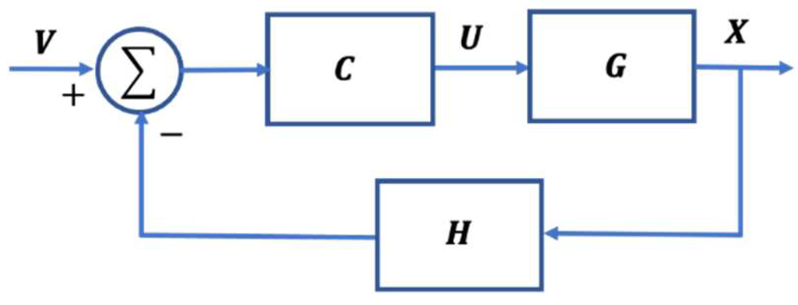
3. The Control Problem
- System:
- Assumptions:
- i.
- Poles (fractional or simple) of the system in Equation (1) can be stable or unstable. However, its zeros are stable. This assumption will be relaxed in future work.
- ii.
- The system is fully observable and controllable. Those that are only partially observable and controllable will be considered in future work.
- Control Problem:
- iii.
- The design of feedback and feedforward compensators required for tracking (a) a unit step and (b) a periodic input is considered (inputs denoted by ). The closed-loop transfer function in each case has the form shown in the equation below (where, ):
- iv.
- The response of a fractional LTI system to is (this is discussed in some detail in Appendix A). However, contrary to integer order systems, is not a polynomial but an expression containing fractional powers of . Fractional systems, therefore, cannot be studied in general using frequency responses. Consequently, closed-loop responses to a randomized periodic input are investigated to assess the generalizability of the compensators designed for iii (b).
- v.
- And finally, the robustness of control designs to input noise and uncertainties in the coefficients and exponents of the system in Equation (1) is presented.
Simulation Tools Used
4. Currently Available Methods for Controlling Fractional LTI Systems
Description of Methods Currently Available
- A.
- Technique 1: Approximate terms involving fractional powers ofusing rational functions. In this method, a standard LTI system approximates the dynamical behavior of a fractional one, which in turn permits the use of methods available for standard systems.
- ○
- ○
- Advantages: The technique can be applied to transfer functions that contain terms with real powers (rational or irrational) of . Both open and closed-loop behaviors of the system can be represented using rational transfer functions.
- ○
- Disadvantages: There are two primary disadvantages to this approach. The first is that approximations using rational transfer functions will, in general, be of a much higher order than the original fractional system. The second is that series connections of rational approximations may lead to incorrect models. For example, . Such limitations could narrow the general applicability of rational approximations.
- B.
- Technique 2: Convert transfer functions that have a common fractional power of () into a polynomial expressed in terms of a new variable. Methods available for standard systems can then be applied to control these systems in the new coordinates (-plane), and results can be transferred back to the -plane.
- ○
- ○
- Advantages: Once the system is converted to the -plane, techniques available for standard systems can be used to study the stability properties of the original fractional ones and to modify their closed-loop behaviors.
- ○
- Disadvantages: This approach suffers from four distinct disadvantages.
- ▪
- First, it cannot be applied to non-commensurate systems (where the fractional power cannot be factored out).
- ▪
- Second, the control design for desired closed-loop behavior is not straightforward. While stability results carry over from -plane to the -plane, control performances may not. In fact, it is shown in Section 6 that good control performance in the -plane does not lead to a similar one in the -plane.
- ▪
- Third, the stability result derived in [29] is a sufficient condition based on the primary solution , and an extension of the De Moivre formula to non-integer exponents (). Together, these were used to argue that the system is unstable only in the cone , and suggest that a fractional system might enjoy an increased stability margin over its standard counterpart .
- -
- The more general formula for complex numbers, however, is , and can lead to roots with physical meaning in higher-order Riemannian sheets. For example, does not have a pole in the first sheet but does so in the second [30].
- -
- Further, is a unique solution only for or . Otherwise, there are multiple ones.
- ▪
- And finally, it is noted that the closed loop transfer function of the system will continue to retain fractional powers of .
- C.
- Technique 3: Extend Technique 2 to transfer functions with rational powers of by expressing them as fractions. They can then be controlled in the same manner as commensurate ones.
- ○
- ○
- Advantages: This method allows any fractional system with rational exponents to be converted to the -plane. Since the technique is restricted to rational exponents, it allows the full use of the extended De Moivre formula.
- ○
- Disadvantages: This approach suffers from the same disadvantages as Technique 2 in terms of stability margins, control performances, and fractional terms in closed-loop transfer functions. In addition, depending on the value of the LCM, conversion from the -plane could lead to high-order functions in the -plane.
- D.
- Technique 4: Apply the control method, which uses a fractional derivative (instead of an ordinary one) and a fractional integral (instead of an ordinary one) in the control law.
- ○
- This method was proposed in 1999 by Podlubny for general fractional LTI systems [18]. It is noted that examples considered have generally been standard second-order systems with additional fractional terms.
- ○
- Advantages: This method extends the well-known PID control technique and can be used for the control of any fractional system represented by a transfer function with terms that have either rational or irrational powers of .
- ○
- Disadvantages: A simple method for the design of the fractional exponents and as well as the gains used in control is not available at present. In addition, the closed loop transfer function of the system will continue to contain fractional powers of .
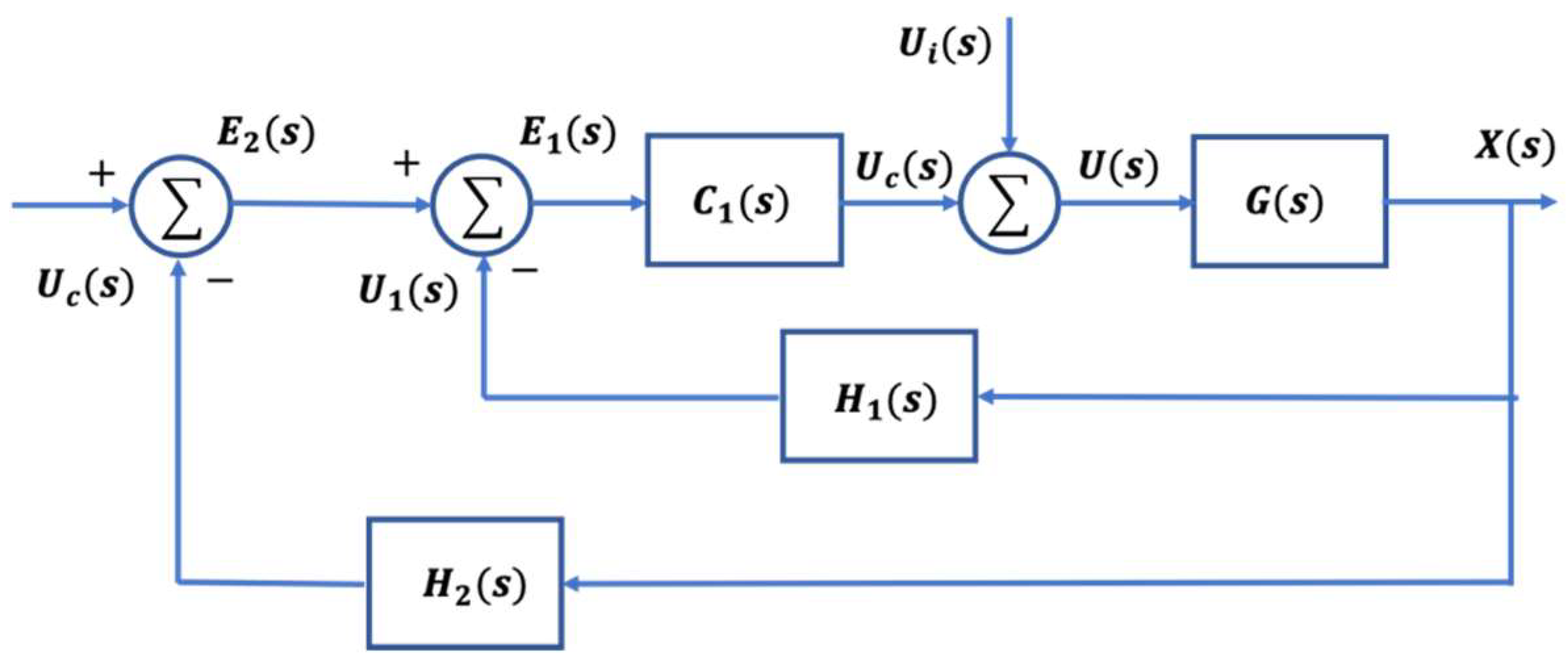
5. Transform and Control: A New Method
- i.
- Transform the fractional system into a standard one using feedback and feedforward compensation (, a rational transfer function. It is shown that this process involves the following two steps:
- a.
- Cancelation of the zeros of a fractional plant in the feedforward path. Since the paper only deals with systems that have stable zeros (a condition that will be relaxed in future work), this pole-zero cancelation step does not involve unstable poles in the feedforward controller. The realization of the transfer functions needed for the cancelation is discussed in Section 8.
- b.
- Transformation of the fractional poles of the system into simple poles using feedback. This step is quite different from pole-zero cancelation and may be thought of as being similar to pole placement in LTI systems theory.
- ii.
- With this step complete, control the transformed system () using widely available tools in linear systems theory to achieve desired closed-loop behavior.

- -
- System 1: , where . The system has a fractional pole at the origin.
- -
- System 2: , where . This moves the fractional pole to -.
- -
- System 3: , where . This adds a fractional zero at the origin.
- -
- System 4: , where . This moves the fractional zero to -.
- -
- System 5: , where and . This is a standard second-order system with additional fractional terms.
Steps Involved in the Application of the New Method
- Choose to change the fractional poles in to simple ones.
- Use to cancel fractional zeros in .
- Use to cancel fractional zeros in .
- Design to achieve desired closed-loop behavior.
6. Control of the System in Section 3 with Currently Available and the New Methods
6.1. Control Simulations
- A.
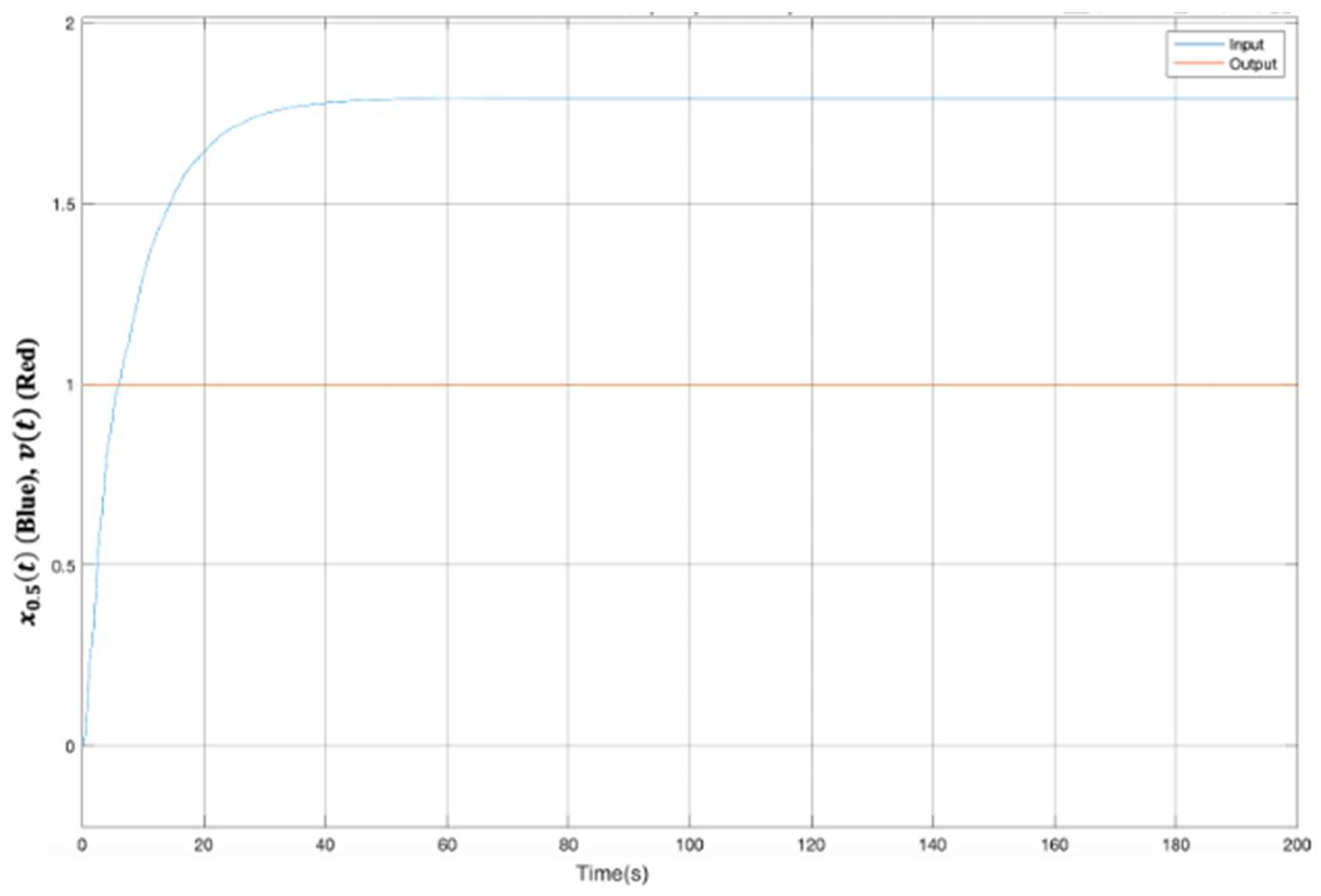
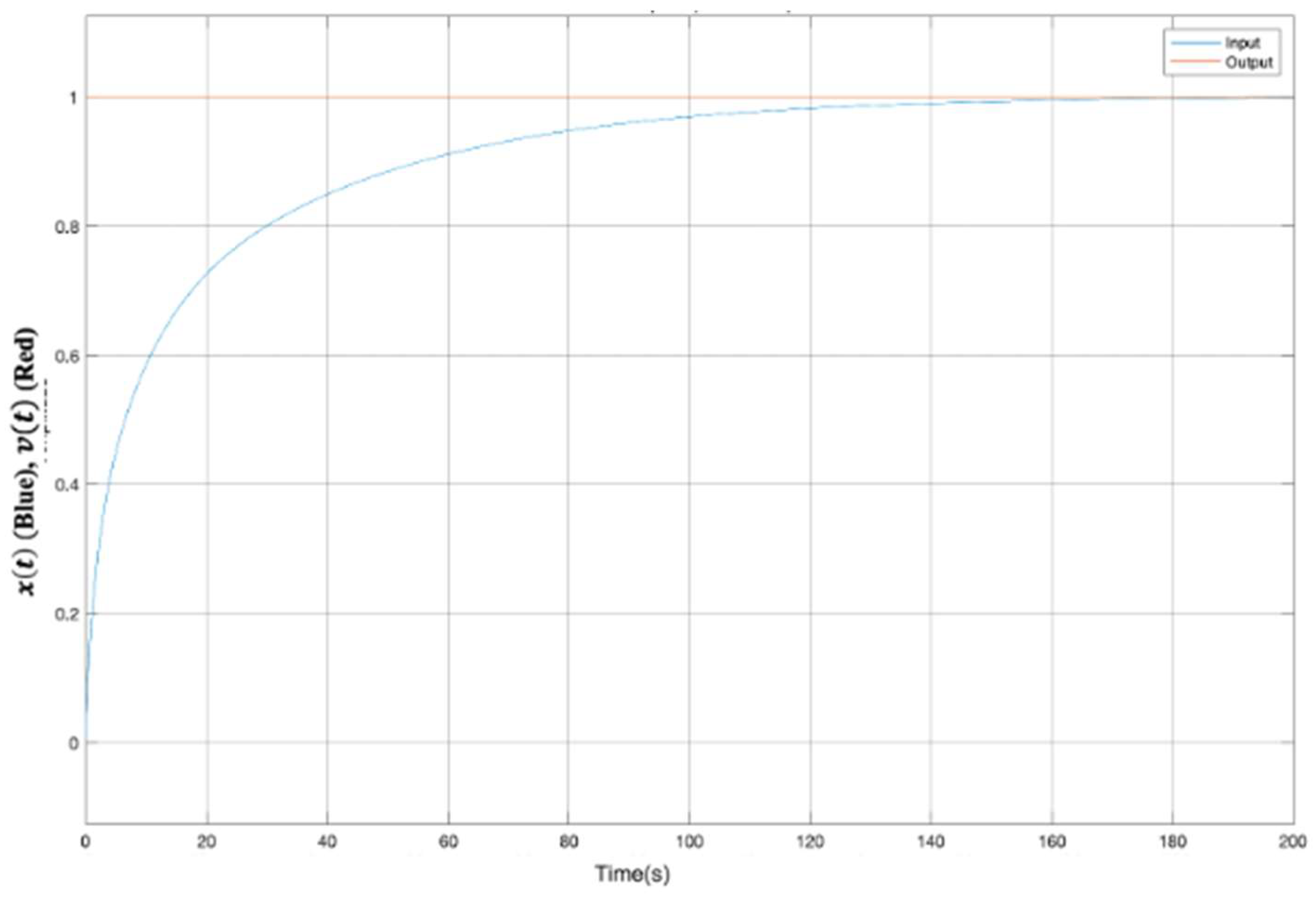
- For step response, the objective is to have the system rapidly reach a steady state behavior of , where is small and is the settling time.
- B.
- For periodic inputs, convergence to is of interest.
- C.
- As stated before, frequency response techniques cannot be used to study the generalizability of control designs used for fractional LTI systems. Therefore, a randomized periodic input will be used instead. The input signal considered here oscillates at frequencies that are randomly selected from the bandwidth of the input in B.
- D.
- For robustness, controllers designed for periodic inputs will be subject to control noise and model uncertainty (both coefficients and exponents).
- Simulation results describe the responses of the closed-loop system to the following:
- i.
- Unit step input.
- ii.
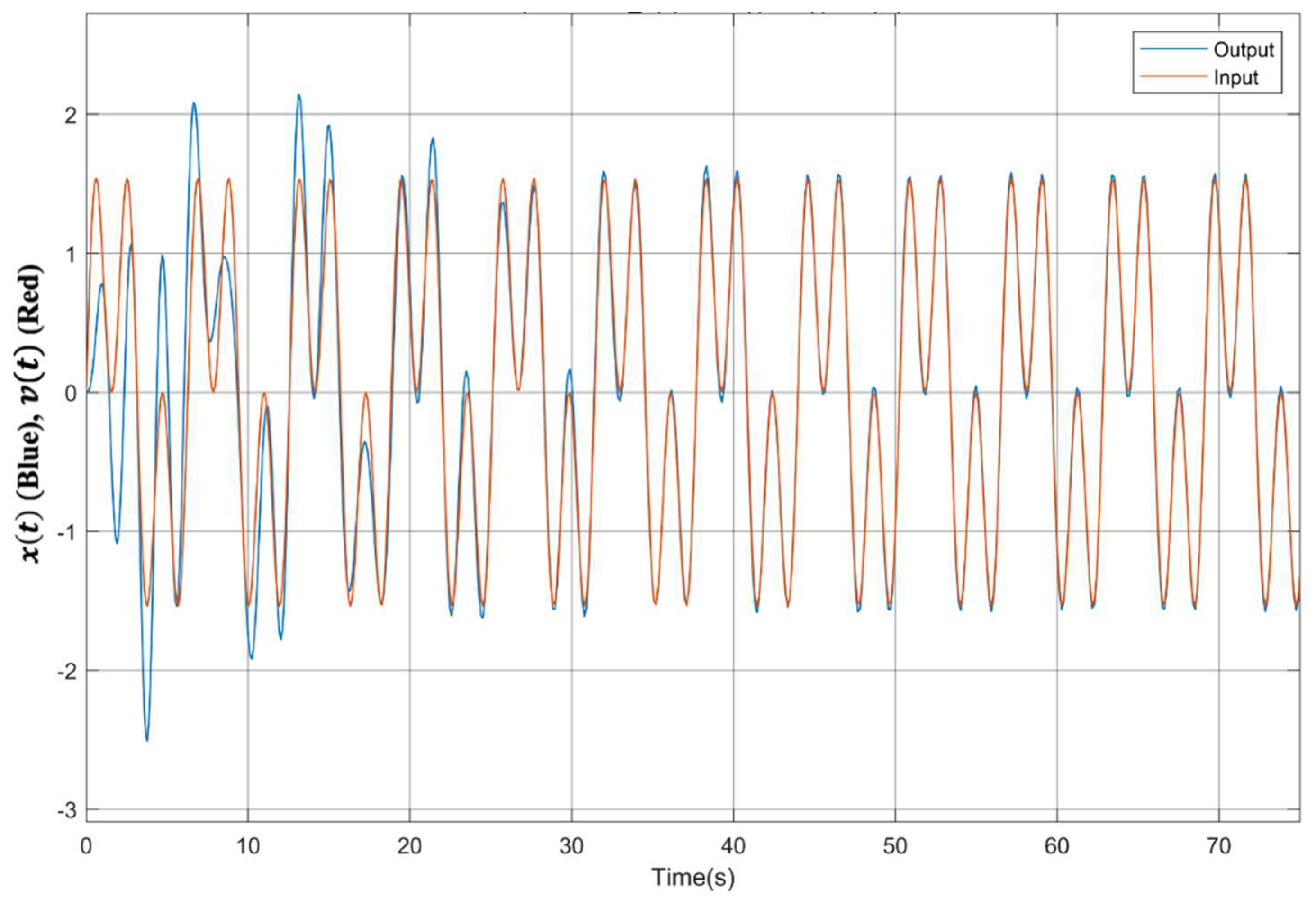
- Periodic input (multiple low-frequency harmonics). The randomized signal will therefore be selected in bandwidth Hz.
6.2. Currently Available Methods
- Technique 1: The system in Equation (4) is controlled using the steps described below:
- -
- and for Step.
- -
- and
- -
- for Periodic.


- Techniques 2 and 3: Since the system in Equation (4) is commensurate, Techniques 2 and 3 are identical. Control of the system can be carried out as shown below:
- -
- and for Step.
- -
- and for Periodic.
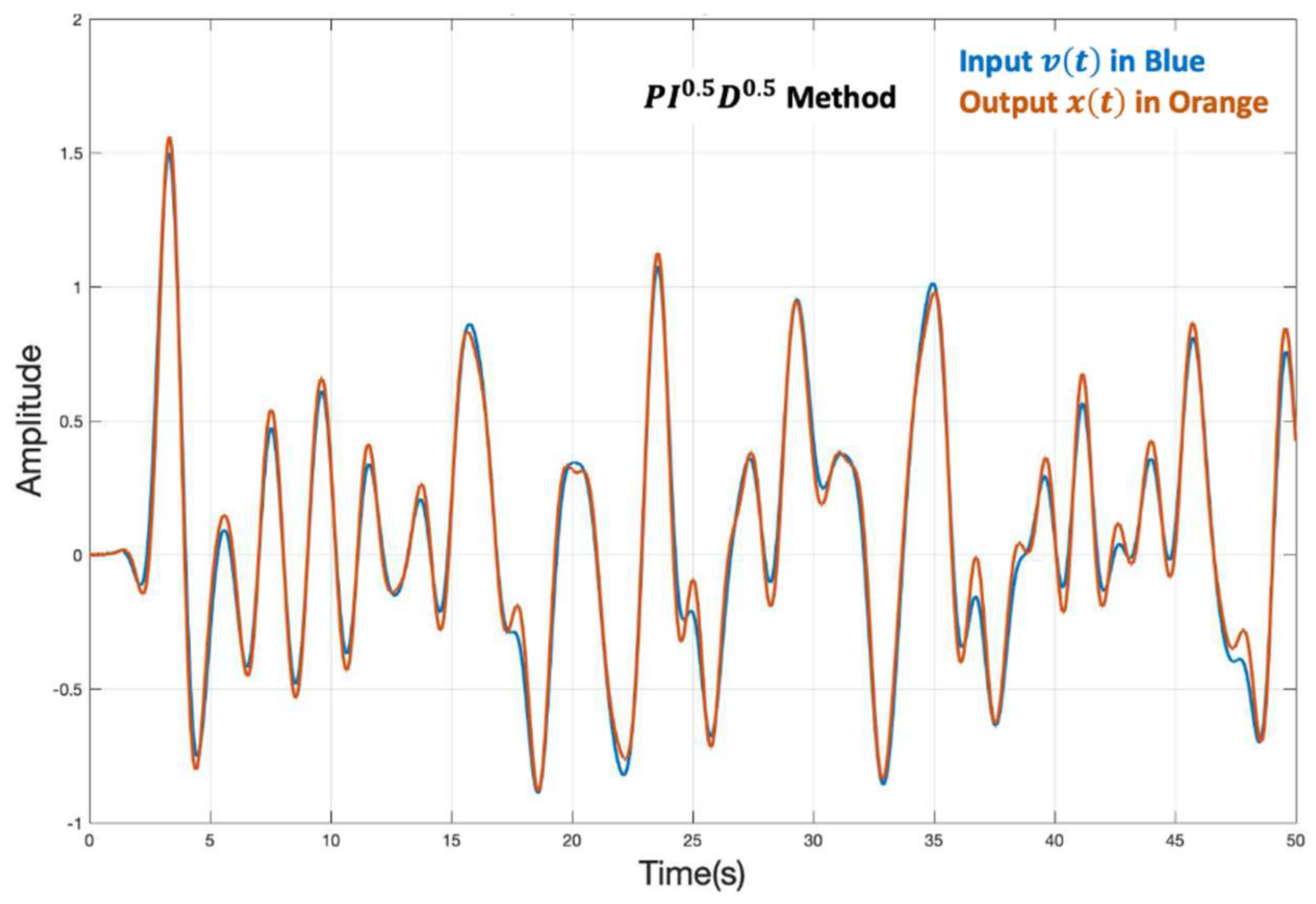
6.3. The New Method
- -
- and for Step.
- -
- and for Periodic.
6.4. Comparison of Closed Loop Responses
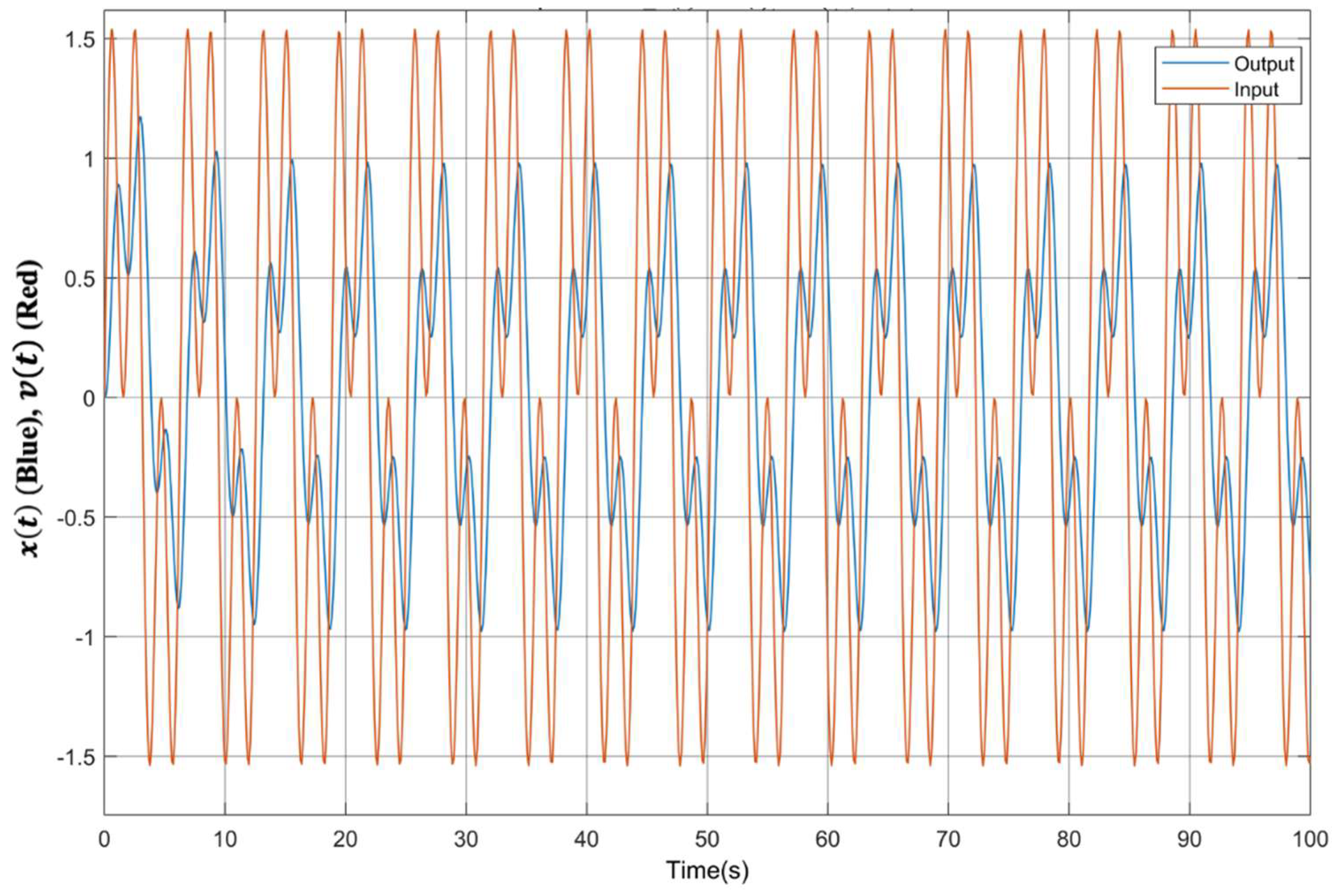
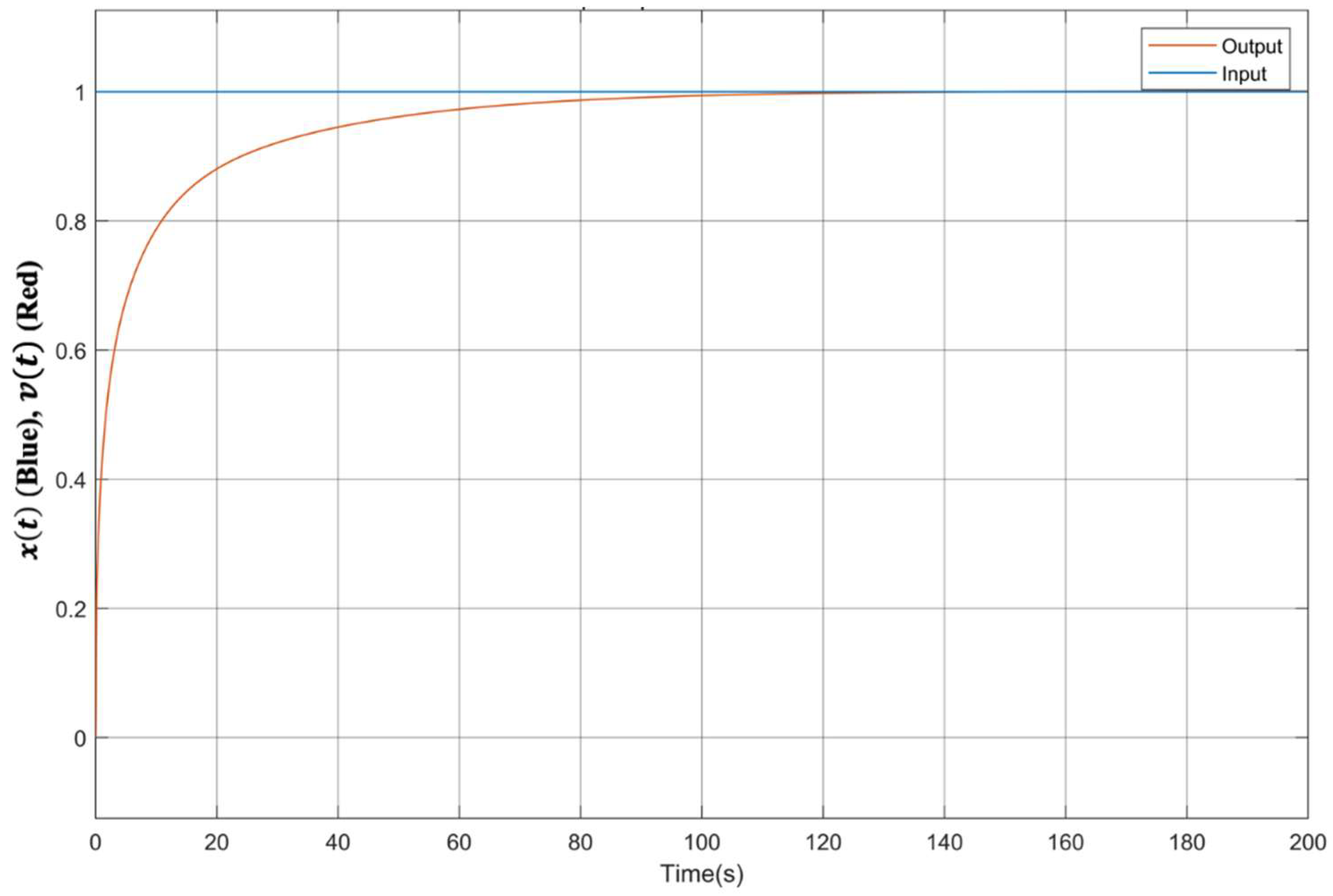
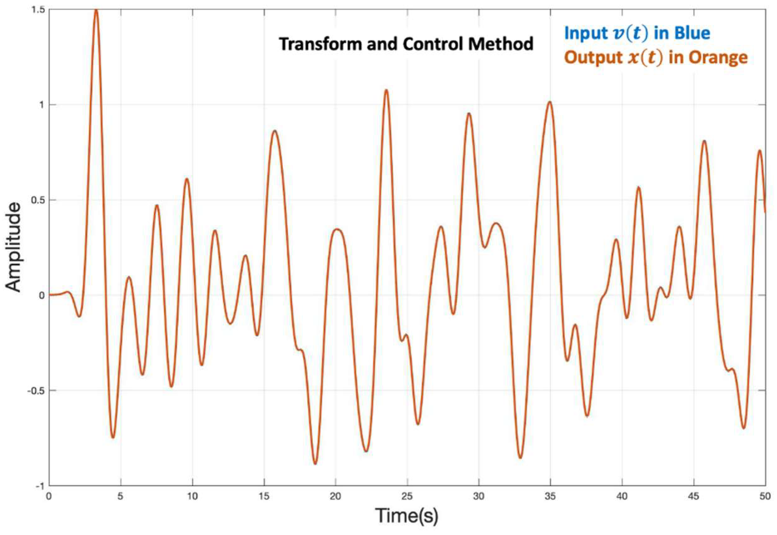
- Closed Loop Responses to Step Input: Convergence to steady-state took many tens of seconds with all currently available methods. Of the four current techniques, control seemed to exhibit the best steady-state behavior. A reasonable steady-state behavior was seen with a rational approximation of the original fractional plant. Techniques 2 and 3 required a control design that exhibited significant steady-state error in the -plane in order to achieve a good response in the -plane. The new method converged rapidly to excellent steady-state behavior with just a gain in the outer feedback loop.
- Closed Loop Responses to Periodic Input: As with step response, convergence to steady-state with a periodic input took many tens of seconds with all currently available methods. The best steady-state behavior was seen with the use of Technique 1. However, a second-order compensator was required for the control performance. control seemed to exhibit reasonable tracking behavior for the component but had difficulties doing so for . Techniques 2 and 3 did not yield good tracking behavior. While control performance was reasonable after prolonged transients (200 s) in the -plane, it was poor in the -plane. The new method converged quickly to excellent steady-state behavior with a first-order outer loop feedback compensator.
- Relationship between Fractional Orders and Compensator Designs: The choice of and in the new method remains the same regardless of the actual values of the fractional terms in the original system. The latter only affected the compensation terms and chosen for the transformation of . For every pair, the transformed system, and the choice of and remained the same.
- Closed Loop Transfer Function: The closed-loop transfer function achieved with the new method for the example is always rational and of second order. With existing techniques, this is not the case. Technique 1 yields a fifth-order rational function. With Techniques 2, 3, and 4, the closed-loop transfer functions are not rational. In fact, they continue to require expressions that contain fractional powers of .
7. Generalizability of Control Designs and Control Robustness
- i.
- Ability to track a periodic input with randomized frequencies between and Hertz, which is the frequency of the component of .
- Comment: It is well known that the Fourier components of the outputs of a standard LTI system will be identical to the ones present in the corresponding inputs. This is due to the fact that it is represented by a rational transfer function. In contrast, a fractional LTI system requires a transfer function with expressions that contain fractional powers of . Consequently, their analyses using frequency responses are not possible. The authors propose, therefore, the study of closed-loop responses to randomized periodic inputs to assess how generalizable control designs may be.
- ii.
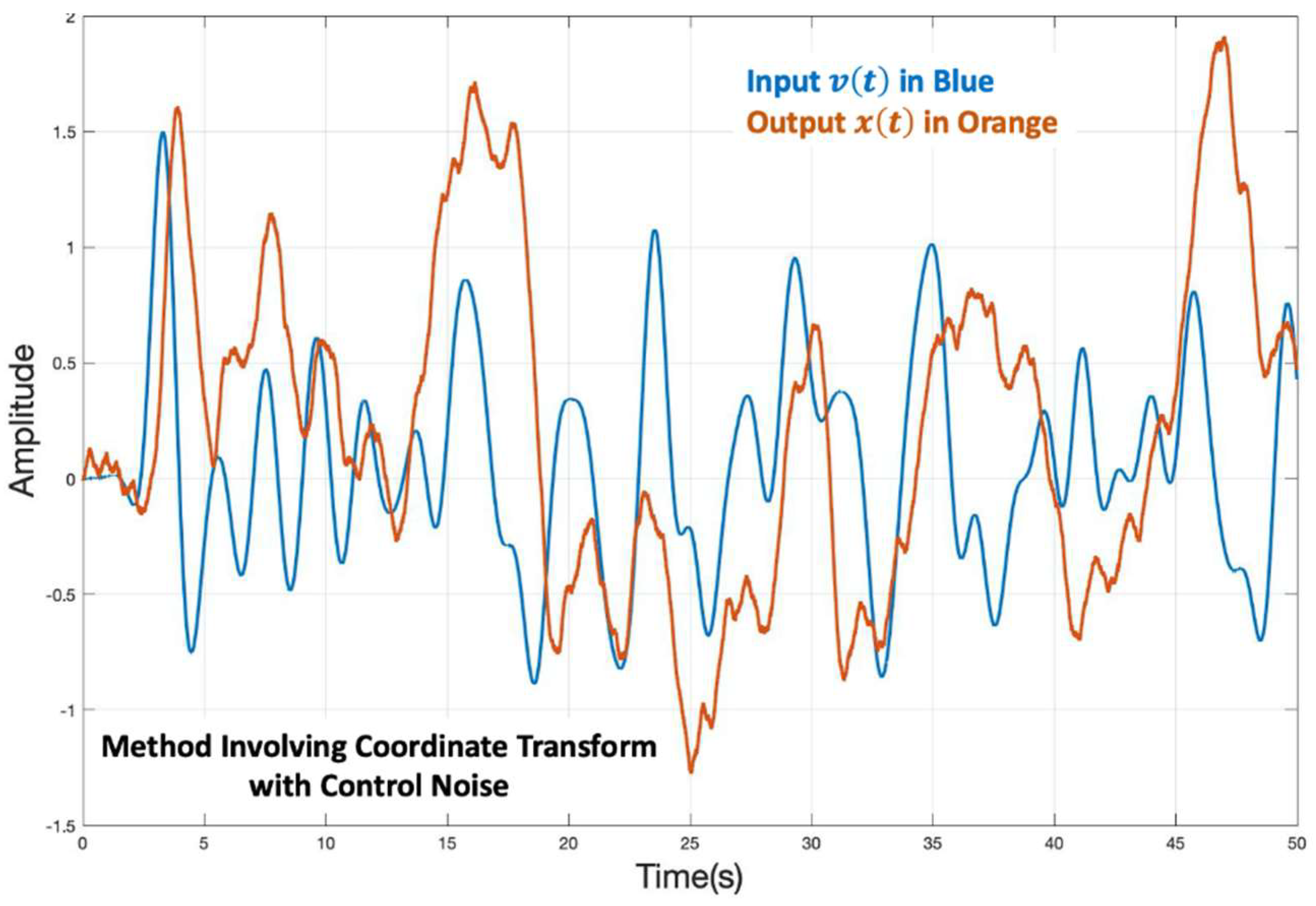
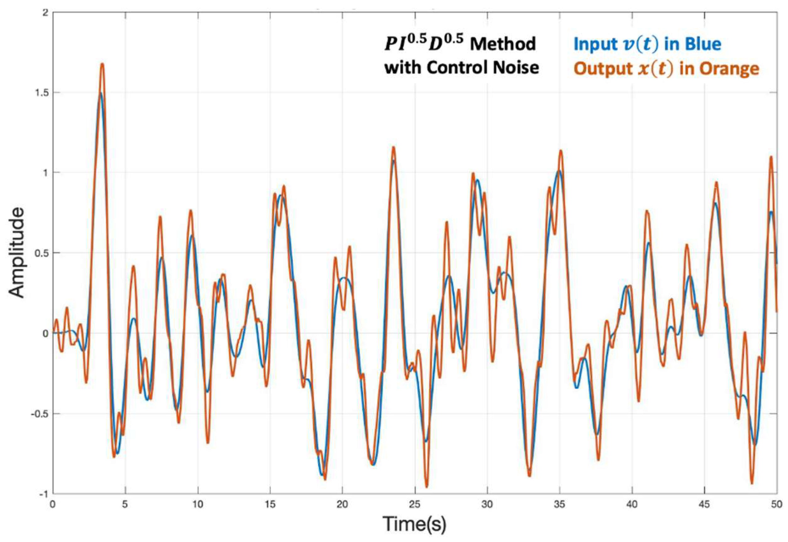
- Closed-loop responses to a randomized periodic input and with control noise bandlimited to 250 Hz (Figure 13). The band limit selected here represents a frequency that is significantly higher than the one used for control designs.
- iii.
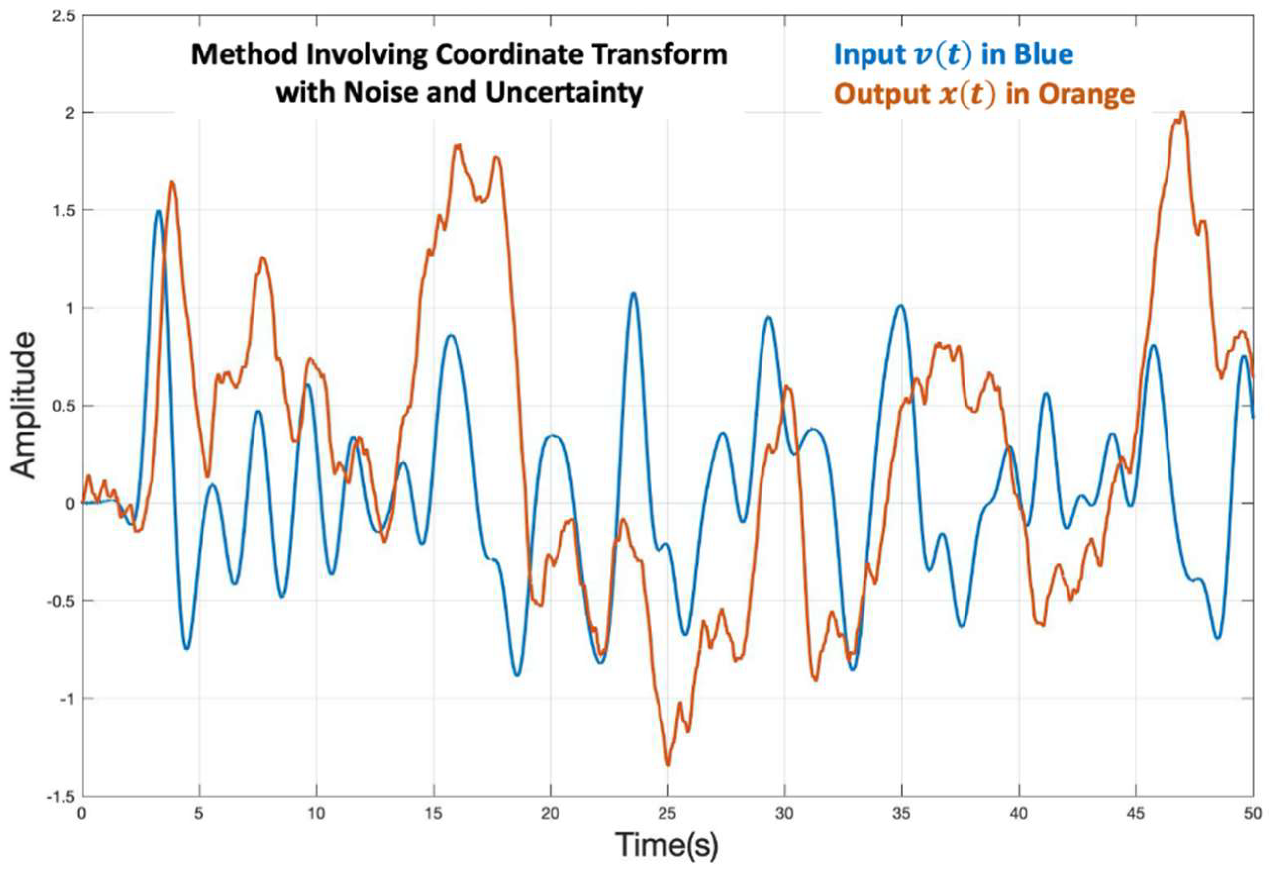
- Closed-loop responses to a randomized input, with control noise and uncertainties in both the coefficients and the fractional exponents of the system in Equation (4).
- Comment: For the purpose of studying the robustness to model uncertainties, the representation of the actual plant (denoted by ) is described as shown below:
- -
- It is assumed that both the estimated and actual plant models are represented by standard LTI systems of second order, with the additional fractional terms (i.e., the structure is the same as shown in Equation (4)).
- -
- Parameters of the estimated and actual models are related as follows: , where is the estimated value of , and is known (i.e., the uncertainty bound for each parameter is known).
- -
- It is assumed in this paper that , where is a random value between . Specifically, the system shown in Equation (5) below is used for the assessment of the robustness of all five control designs (the four currently available and the new method)
7.1. Control Analysis
- A.
- For randomized periodic inputs, is once again of interest.
- B.
- For robustness to noise, convergence to will be assessed with the noise signal Figure 13 added to the control input.
- C.
- For robustness to noise and uncertainties, noise is added to the input to the plant model in Equation (5) (to account for the differences between estimated and actual plant models), and convergence to will be assessed.
- Generation of Randomized Periodic Inputs
- Technique 1:
- Techniques 2 and 3:
- Technique 4:
- New Method:
7.2. Comparison of Closed Loop Responses
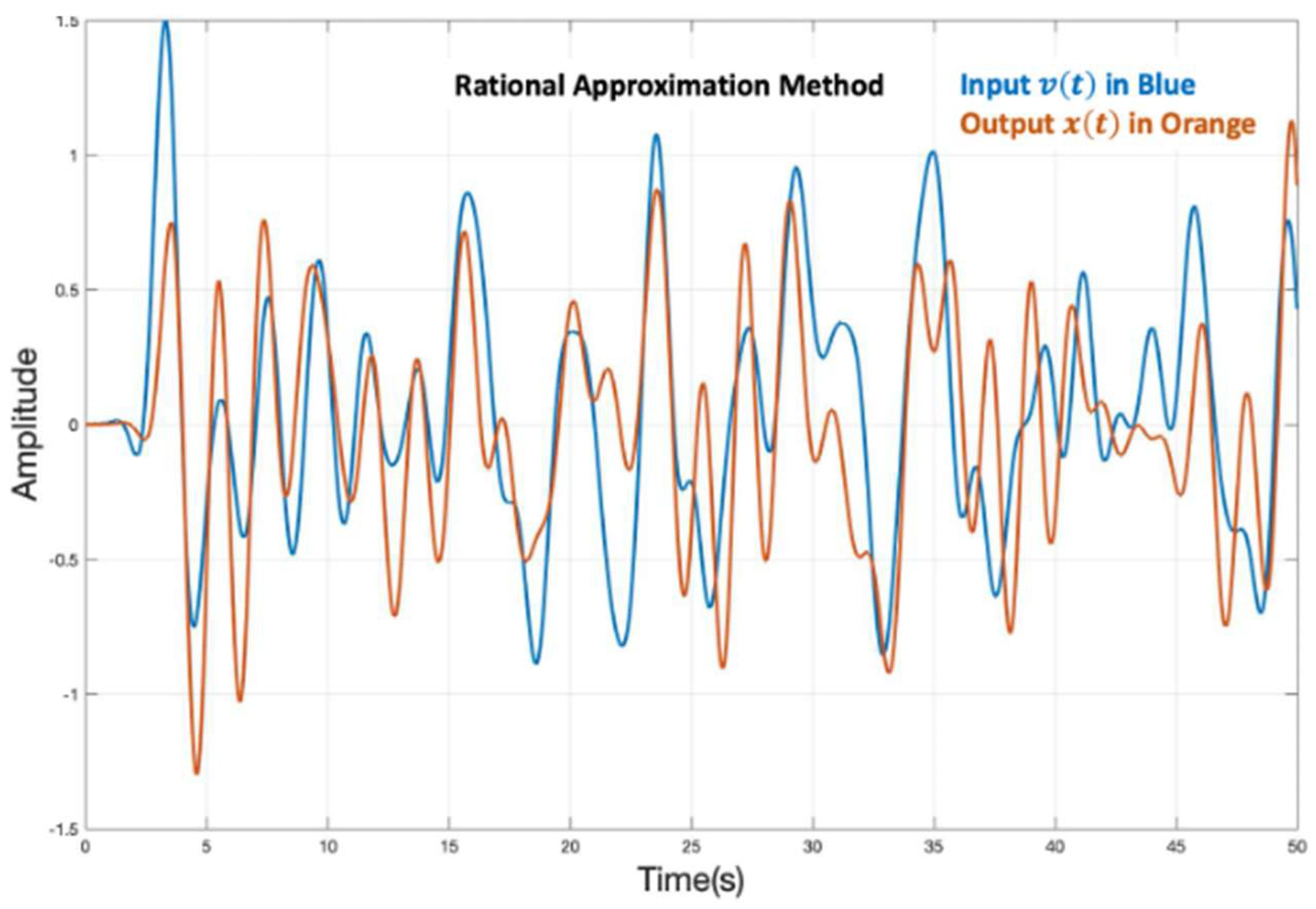
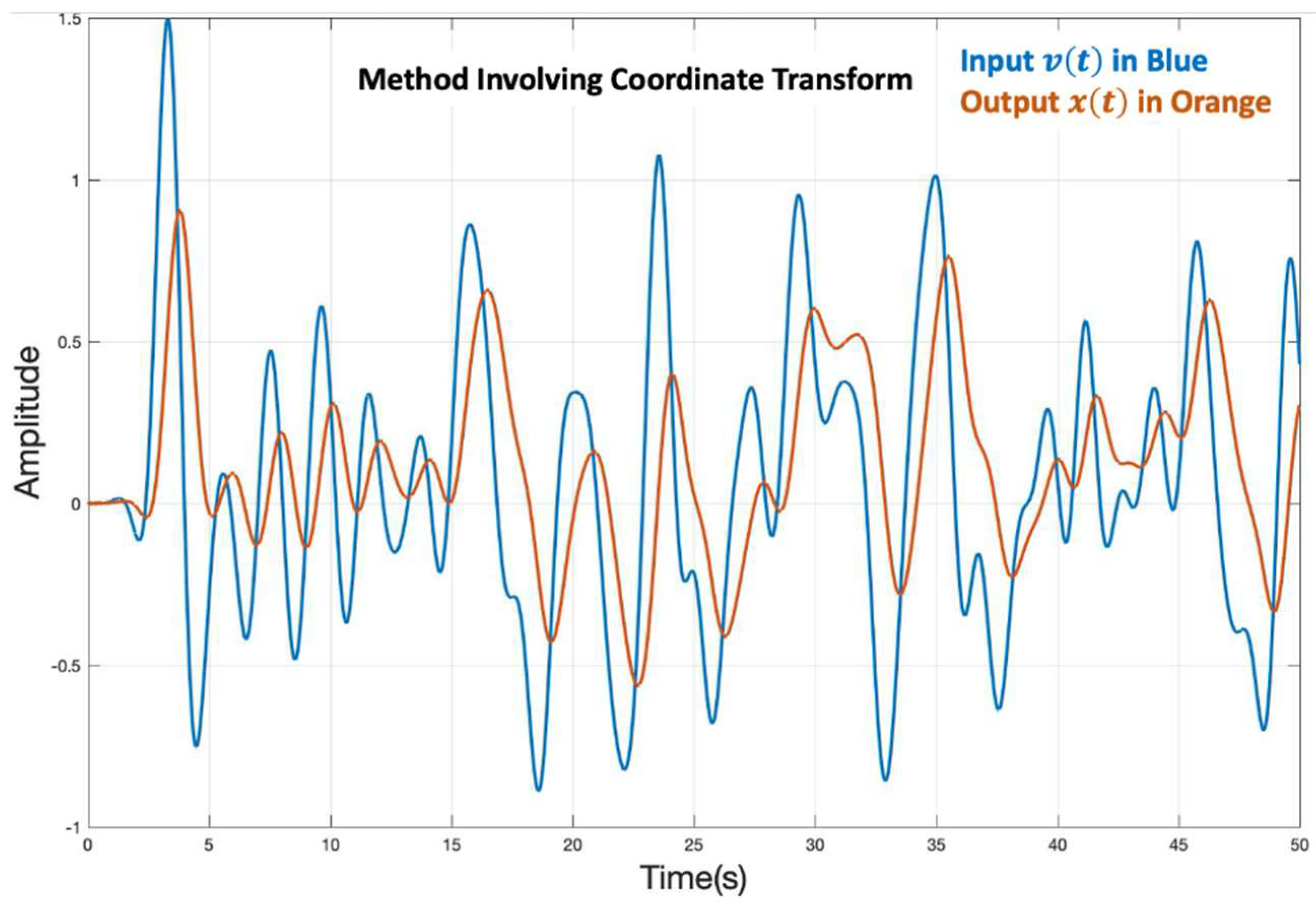
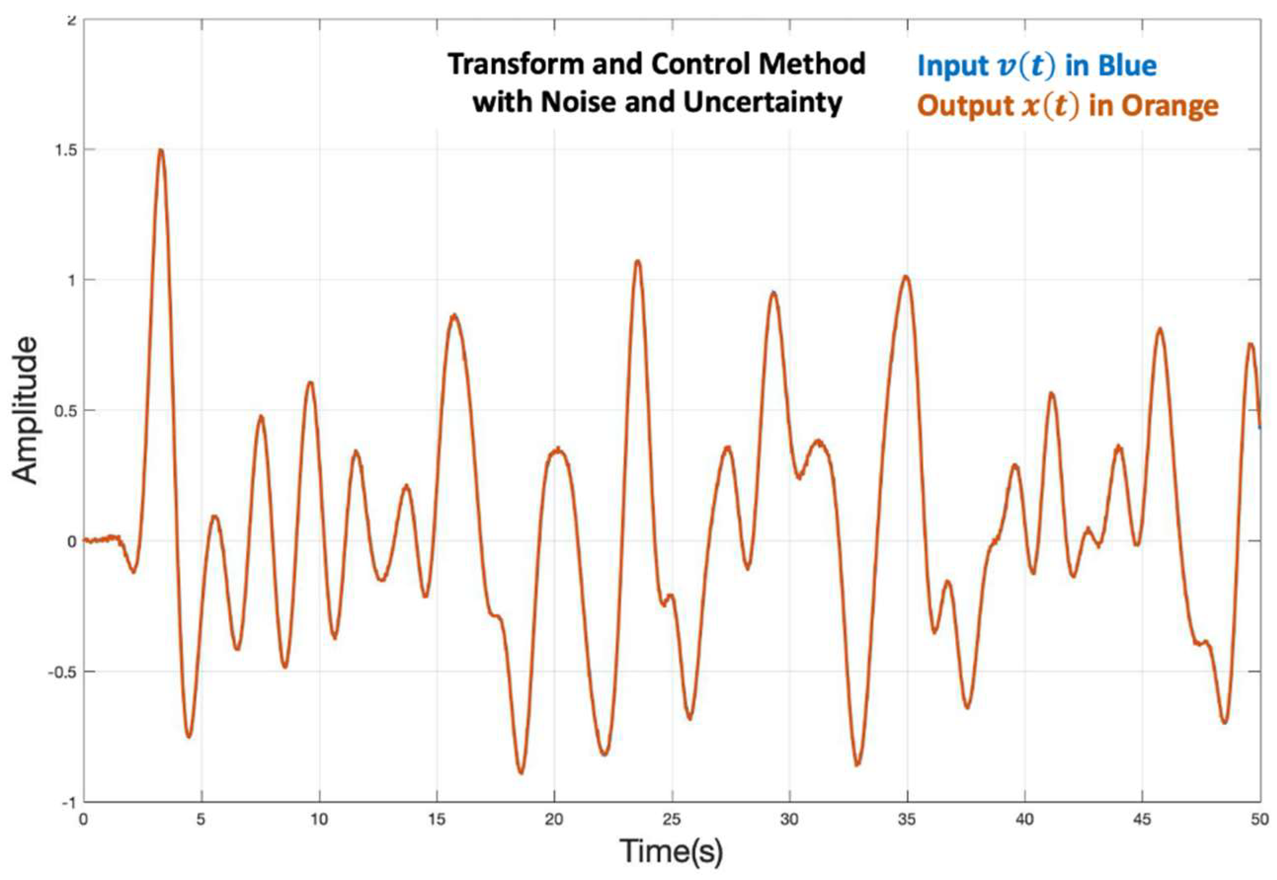
- Closed Loop Responses to Periodic Input: Convergence to a neighborhood of the steady state could not be achieved with the use of Techniques 1, 2, and 3. Technique 4 exhibited large steady-state errors, while the new method showed excellent convergence and negligible steady-state behavior.
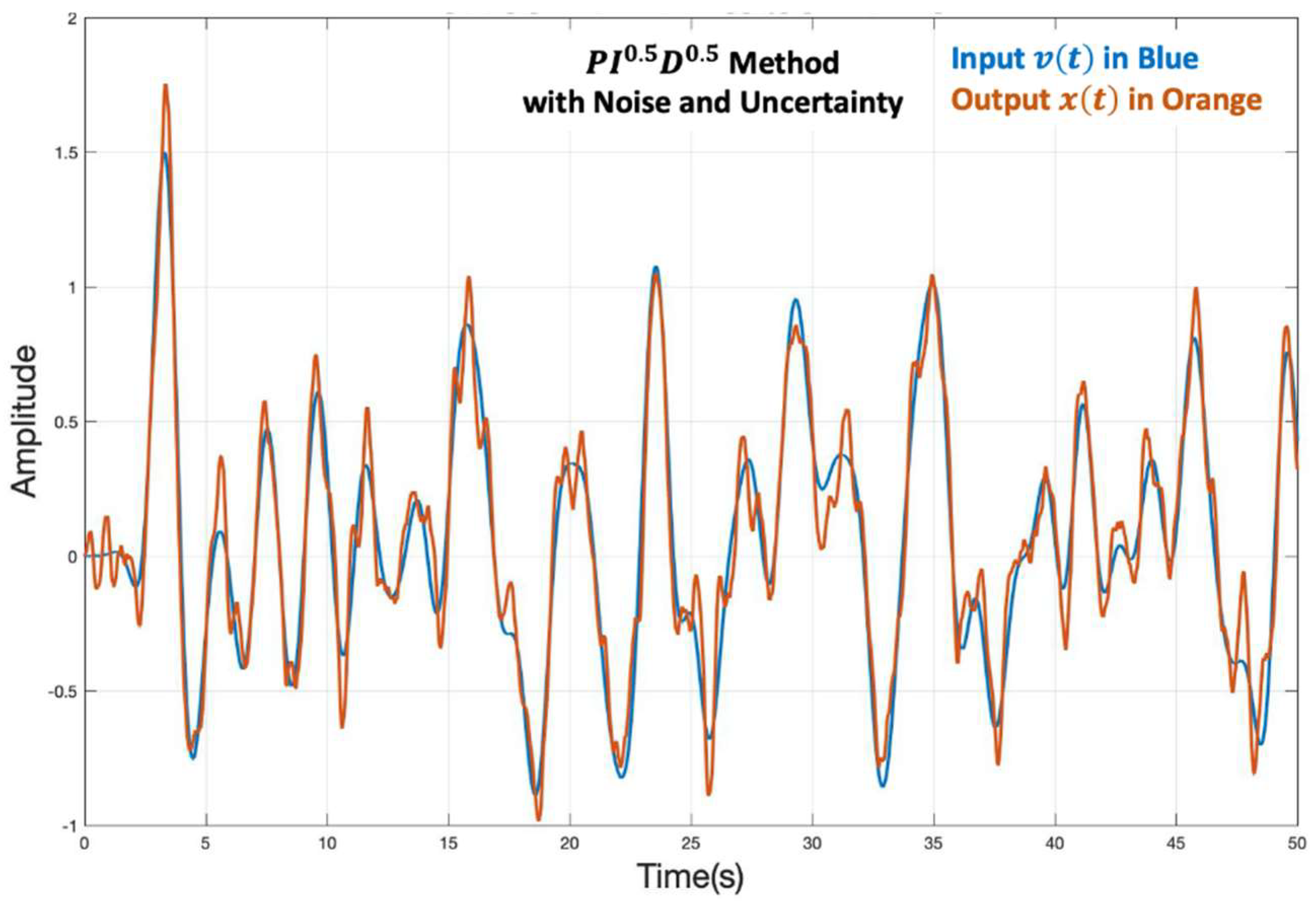
- Robustness to Control Noise: Control noise had a significant impact on the tracking performance of all currently available techniques in the bandwidth of the input signal. The new method showed excellent robustness in controlling noise. Some amount of chatter was seen in the closed-loop response. Future work will focus on smoothing this.
- Robustness to Parameter Uncertainty: Uncertainties in the coefficients and the exponents of the plant had a significant impact on the tracking performance of all currently available techniques in the bandwidth of the input signal. The new method showed excellent robustness to such uncertainties.
8. Realization of the Fractional Compensation Terms Used in the New Method
- Existence
- Realization of Fractional Terms
- Realization of Feedback and Feedforward Compensation Transfer Functions
9. Applicability of the New Method to Systems with Arbitrary Initial Conditions
- Realization of
10. Conclusions and Future Work
Author Contributions
Funding
Institutional Review Board Statement
Informed Consent Statement
Conflicts of Interest
Appendix A
- Linear Systems Theory
- The Laplace Transform in Linear Systems Theory
- Integer (vs) Fractional Order Derivative
- Origin of the Fractional Order Derivative
- The Riemann-Liouville Derivative
- Caputo Fractional Derivative
- Rationale for the Selection of the Caputo Definition
- Other Definitions of a Fractional Derivative
- Fractional LTI Systems


- i.
- The denominator of is less than that of for small values of .
- ii.
- is multiplied by , which is large for small values of .
- Study of Fractional LTI Systems Using the Laplace Transform
- It can be shown that is an eigenfunction of the system in Equation (A9) since the convolution operation involved in studying the response of the system to (with integration limits ), allows the Gamma function to be factored out. As a result, the Laplace transform can be applied for the analysis (and control) of fractional LTI systems.
- Ordinary derivatives and integrals are typically defined in the Riemann sense. On the other hand, with fractional systems, both the derivatives and integrals involve convolutions with power kernels that are singular at one of the two integration limits. However, contrary to the discussions in [51] (and other similar ones), this is not seen as an issue by the authors since such convolutions can be defined and do exist in the Lebesgue sense.
- And lastly, by applying the results discussed in [38] it can be shown that the Laplace transform of the Caputo derivative (which involves a Lebesgue convolution) exists. It is noted that the condition must be true since exists only when . This additional restriction is required for the analysis of fractional LTI systems using the Laplace transform. Therefore, the interpretation of must be , which in turn requires that is sufficiently differentiable.
- A Note on Input-Output Behavior of Fractional LTI Systems
Appendix B

- System 1: Fractional Integrator:
- System 2: One Fractional Pole:
- System 3: One Fractional Pole and A Fractional Zero at the Origin:
- System 4: One Fractional Pole and One Fractional Zero:
- System 5: Many Fractional Poles and Many Fractional Zeros: :
References
- van Assche, K.; Valentinov, V.V.G. Special Issue on Ludwig von Bertalanffy; Wiley: Hoboken, NJ, USA, 2019; Volume 36, Available online: https://onlinelibrary.wiley.com/toc/10991743a/2019/36/3 (accessed on 21 October 2022).
- Shastri, S.V.; Narendra, K.S. Applications Involving Dynamical Phenomena Described by Fractional Order Derivatives; Yale Technical Report#2002; Yale University Press: New Haven, CT, USA, 2020. [Google Scholar]
- Shastri, S.V.; Narendra, K.S. Fractional Order Derivatives: An Introduction; Yale Technical Report #2001; Yale University Press: New Haven, CT, USA, 2020. [Google Scholar]
- Das, S. Importance of Fractional Calculus in Real Life Engineering and Science Applications. In Proceedings of the Workshop on Fractional Order Systems, Indian Institute of Technology, Kharagpur, India, 16–20 February 2018. [Google Scholar]
- Bagley, R.L.; Torvik, P.J. A Theoretical Basis for the Application of Fractional Calculus to Viscoelasticity. J. Rheol. 1983, 27, 201–210. [Google Scholar] [CrossRef]
- Dai, Z.; Peng, Y.; Mansy, H.; Sandler, R.; Royston, T. A Model of Lung Parenchyma Stress Relaxaton Using Fractional Viscoelasticity. Med. Eng. Phys. 2015, 37, 752–758. [Google Scholar] [CrossRef] [PubMed]
- Astrom, K.J.; Murray, R.M. Feedback Systems: An Introduction to Scientists and Engineers; Princeton University Press: Princeton, NJ, USA, 2009. [Google Scholar]
- Boskovic, M.; Sekara, T.; Lutovac, B.; Mandic, P. Analysis of Electrical Circuits including Fractional Order Elements. In Proceedings of the 6th Mediterranean Conference on Embedded Computing, Bar, Montenegro, 11–15 June 2017. [Google Scholar]
- Magin, R.L. Fractional calculus models of complex dynamics in biological tissues. Comput. Math. Appl. 2010, 59, 1586–1593. [Google Scholar] [CrossRef] [Green Version]
- Rabiee, R.; Chae, Y. Adaptive Base Isolation System to Achieve Structural reiliency under Both Short- and Long-Period Earthquake Motions. J. Intell. Mater. Syst. Struct. 2018, 30, 16–31. [Google Scholar] [CrossRef]
- Shahi, S.; Baker, J. An Efficient Algorithm to Identify Strong-Velocity Pulses in Muticomponent Ground Motions. Bull. Seismol. Soc. Am. 2014, 104, 2456–2466. [Google Scholar] [CrossRef]
- Makris, N.; Constantinou, M. Spring-Viscous Damper Systems for Combined Seismic and Vibration Isolation. Earthq. Eng. Struct. Dyn. 1992, 21, 649–664. [Google Scholar] [CrossRef]
- Sabatier, J.; Merveillaut, M.; Francisco, J.; Guillemard, F.; Porcelatto, D. Lithium-Ion Batteries Modeling Involving Fractional Differentiation. J. Power Sources 2014, 262, 36–43. [Google Scholar] [CrossRef]
- Xue, D. Fractional-Order Control Systems: Fundamental and Numerical Implementations; De Gruyter Academic Publishing: New York, NY, USA, 2017. [Google Scholar]
- Oustaloup, A. Systemes Asservis Lineaires d’Ordre Fractionnaire: Theorie et Pratique; Editions Masson: Paris, France, 1983. [Google Scholar]
- Petras, I. Stability of Fractional-Order Systems with Rational Orders. arXiv 2008, arXiv:0811.4102v2. [Google Scholar]
- Li, Z.; Liu, L.; Dehghan, S.; Chen, Y.; Xue, D. A Review and Evaluation of Numerical Tools for Fractional Calculus and Fractional Order Controls. Int. J. Control. 2015, 90, 1165–1181. [Google Scholar] [CrossRef] [Green Version]
- Podlubny, I. Fractional Order Systems and Controllers. IEEE Trans. Autom. Control. 1999, 44, 208–214. [Google Scholar] [CrossRef]
- Vinagre, B.; Podlubny, I.; Hernandez, A.; Feliu, V. Some Approximations of Fractional-Order Operators Used in Control Theory. Fract. Calc. Appl. Anal. 2000, 3, 231–248. [Google Scholar]
- Shastri, S.V.; Narendra, K.S. Transform and Control: A New Approach to Controlling Dynamical Systems Described by Fractional Order Derivatives; Yale Technical Report #2003; Yale University Press: New Haven, CT, USA, 2020. [Google Scholar]
- Birs, I.; Muresan, C.; Nascu, I.; Ionescu, C. A Survey of Recent Advances in Fractional Order Control for Time Delay Systems. IEEE Access 2019, 7, 30951–30965. [Google Scholar] [CrossRef]
- Sabatier, J.; Moze, M.; Farges, C. LMI Stability Conditions for Fractional Order Systems. Comput. Math. Appl. 2010, 59, 1594–1609. [Google Scholar] [CrossRef]
- Padula, F.; Visioli, A. Advances in Robust Fractional Control; Springer: New York, NY, USA, 2015. [Google Scholar]
- Ortigueira, M.; Bengochea, G. Non-Commensurate Fractional Linear Systems: New Results. J. Adv. Res. 2020, 11, 11–17. [Google Scholar] [CrossRef]
- Aguila-Camacho, N.; Duarte-Mermoud, M.A.; Gallegos, J.A. Lyapunov Functions for Fractional Order Systems. Commun. Nonlinear Sci. Numer. Simul. 2014, 19, 2951–2957. [Google Scholar] [CrossRef]
- Carlson, G.E.; Halijak, C.A. Approximation of a Fractional Capacitor (1/s)^(1/n) by a Regular Newton Process. IEEE Trans. Circuit Theory CT-11 1964, 2, 210–213. [Google Scholar] [CrossRef]
- Matsuda, K.; Fujii, H. H-Infinity Optimized Wave-Absorbing Control: Analytical and Experimental Results. J. Guid. Control. Dyn. 1993, 16, 1146–1153. [Google Scholar] [CrossRef]
- Krishna, B.T. Studies on Fractional Order Differentiators and Integrators: A Survey. Signal Process. 2011, 91, 386–426. [Google Scholar] [CrossRef]
- Matignon, D. Stability Properties for Generalized Fractional Differential Systems. ESIAM Proc. Fract. Differ. Syst. Model. Methods Appl. 1998, 5, 145–158. [Google Scholar] [CrossRef] [Green Version]
- Lorenzo, C.F.; Hartley, T.T. Generalized Functions for Fractional Calculus; NASA Technical Report—1999-209424/Rev1; NASA: Cleveland, OH, USA, 1999.
- Grosdidier, P.; Morari, M. Interaction Measures under Decentralized Control. Automatica 1986, 22, 309–319. [Google Scholar] [CrossRef]
- Lee, J.; Edgar, T.F. Phase Conditions for Stability of Multi-loop Control Systems. Comput. Chem. Eng. 2000, 23, 1623–1630. [Google Scholar] [CrossRef]
- Gorenflo, R.; Kilbas, A.; Mainardi, F.; Rogosin, S. Mittag-Leffler Functions, Related Topics and Applications; Springer Mongraphs in Mathematics; Springer: New York, NY, USA, 2014. [Google Scholar]
- Bagley, R.; Torvik, P. Fractional Calculus—A Different Approach to the Analysis of Viscoelastically Damped Structures. AIAA J. 1983, 21, 5741–5748. [Google Scholar] [CrossRef]
- Chen, Y.-Q. Ubiquitous Fractional Order Controls? IFAC Proc. Vol. 2006, 39, 481–492. [Google Scholar] [CrossRef] [Green Version]
- Dastjerdi, A.A.; Vinagre, B.M.; Chen, Y.-Q.; Hossein Nia, S.H. Linear Fractional Order Controllers; A Survey in the Frequency Domain. Annu. Rev. Control. 2019, 47, 51–70. [Google Scholar] [CrossRef]
- Lizorkin, P. Fractional Integration and Differentiation. In Encyclopedia of Mathematics; Kluwer Academic Publishers: New York, NY, USA, 2001. [Google Scholar]
- Benedetto, J. The Laplace Transform of Generalized Functions. Can. J. Math. 2018, 18, 357–374. [Google Scholar] [CrossRef]
- Daou, R.A.Z.; Francis, C.; Moreau, X. Synthesis and Implementation of Non-Integer Integrators using RLC Devices. Int. J. Electron. 2009, 96, 1207–1223. [Google Scholar] [CrossRef]
- Dimeas, I.; Tsirimokou, G.; Psychalinos, C.; Elwakil, A. Realization of Fractional-Order Capacitor and Inductor Emulators Using Current Feedback Operational Amplifiers. In Proceedings of the International Symposium on Nonlinear Theory and Applications, Kowloon, Hong Kong, China, 1–4 December 2015. [Google Scholar]
- Petras, I.; Chen, Y.; Coopmans, C. Fractional-Order Memristive Systems. In Proceedings of the IEEE Conference on Emerging Technologies and Factory Automation, Mallorca, Spain, 22–25 September 2009. [Google Scholar]
- Krishna, B.; Reddy, K. Active and Passive Realization of Fractance Device of Order ½; Hindawi Publishing (Active and Passive Electronic Components): London, UK, 2008. [Google Scholar] [CrossRef] [Green Version]
- Gonzalez, E.; Dorcak, L.; Monje, C.; Valsa, J.; Caluyo, F.; Petras, I. Conceptual Design of a Selectable Fractional-Order Differentiator for Industrial Applications. Fract. Calc. Appl. Anal. 2014, 17, 697–716. [Google Scholar] [CrossRef] [Green Version]
- Oppenheim, A. Digital Signal Processing; OpenCourseWare; Massachusetts Institute of Technology MIT: Cambridge, MA, USA, 2011; Available online: https://ocw.mit.edu (accessed on 21 October 2022).
- Callier, F.M.; Desoer, C.A. Linear Systems Theory; Springer: New York, NY, USA, 1991. [Google Scholar]
- Bryson, J.A.E.; Ho, Y.-C. Applied Optimal Control; Taylor & Francis: New York, NY, USA, 1975. [Google Scholar]
- Zhou, K.; Doyle, J. Essentials of Robust Control; Prentice Hall: New York, NY, USA, 1998. [Google Scholar]
- Narendra, K.S.; Annaswamy, A.M. Stable Adaptive Systems; Prentice-Hall: New York, NY, USA, 1989. [Google Scholar]
- Ross, B. The Development of Fractional Calculus 1695–1900. Hist. Math. 1977, 4, 75–89. [Google Scholar] [CrossRef] [Green Version]
- Caputo, M. Linear Model of Dissipation whose Q is almost Frequency Independent. Geophys. J. Int. 1967, 13, 529–539. [Google Scholar] [CrossRef]
- Sabatier, J. Non-Singular Kernels for Modelling Power Law Type Long Memory Behaviours and Beyond. Cybern. Syst. 2020, 51, 383–401. [Google Scholar] [CrossRef]
- Reimann, B. Versuch einer allgemeinen Auffassung der Integration und Differentiation; Cambridge University Press: Cambridge, UK, 1876. [Google Scholar]
- Mainardi, F. An Historical Perspective on Fractional Calculus in Linear Viscoelasticity. Fract. Calc. Appl. Anal. 2012, 15, 712–717. [Google Scholar] [CrossRef]
- Gorenflo, R.; Mainardi, F. Fractional Calculus and Special Functions; Lecture Notes on Mathematical Physics; University of Bologna: Bologna, Italy, 2007. [Google Scholar]
- Podlubny, I. Fractional Differential Equations; Academic Press: New York, NY, USA, 2009. [Google Scholar]
- Jumarie, G. On the Representation of Fractional Brownian Motion as an integral with respect to (dt)^Alpha. Appl. Math. Lett. 2005, 18, 739–748. [Google Scholar] [CrossRef] [Green Version]
- Jumarie, G. Modified Riemann-Liouville Derivative and Fractional Taylor Series of Nondifferentiable Functions: Further Results. Comput. Math. 2006, 51, 1367–1376. [Google Scholar] [CrossRef]
- Erdelyi, A.; Magnus, W.; Oberhettinger, F.; Tricomi, F. Higher Transcendental Functions; McGraw-Hill: New York, NY, USA, 1955; Volume 3, pp. 206–212. [Google Scholar]
- Mainardi, F. On Some Properties of the Mittag-Leffler Function E_alpha(-t^alpha), Completely Monotone for t > 0 with 0 < alpha < 1. Discret. Contin. Dyn. Syst. Ser. B 2014, 19, 2267–2278. [Google Scholar]
- Luchko, Y.; Gorenflo, R. An Operational Method for Solving Fractional Differential Equations with the Caputo Derivatives. Acta Math. Vietnam 1999, 24, 207–233. [Google Scholar]
- Mikusinski, J. Operational Calculus; Pergamon Press: New York, NY, USA, 1959. [Google Scholar]


| G(s) | H1(s) | C1(s) |
|---|---|---|
 |  | 1 |
 |  | 1 |
 |  |  |
 |  |  |
 |  |  |
| G(s) | H2(s) | C2(s) |
|---|---|---|
 | (p − 1) |  |
 | (p − 1) |  |
 | (p − 1) |  |
 | (p − 1) |  |
 | (p1p2 – a0) + (p1 + p2)s |  |
Disclaimer/Publisher’s Note: The statements, opinions and data contained in all publications are solely those of the individual author(s) and contributor(s) and not of MDPI and/or the editor(s). MDPI and/or the editor(s) disclaim responsibility for any injury to people or property resulting from any ideas, methods, instructions or products referred to in the content. |
© 2022 by the authors. Licensee MDPI, Basel, Switzerland. This article is an open access article distributed under the terms and conditions of the Creative Commons Attribution (CC BY) license (https://creativecommons.org/licenses/by/4.0/).
Share and Cite
Shastri, S.V.; Narendra, K.S.; Zheng, L. A New Method for Controlling Fractional Linear Systems. Fractal Fract. 2023, 7, 50. https://doi.org/10.3390/fractalfract7010050
Shastri SV, Narendra KS, Zheng L. A New Method for Controlling Fractional Linear Systems. Fractal and Fractional. 2023; 7(1):50. https://doi.org/10.3390/fractalfract7010050
Chicago/Turabian StyleShastri, Subramanian V., Kumpati S. Narendra, and Lihao Zheng. 2023. "A New Method for Controlling Fractional Linear Systems" Fractal and Fractional 7, no. 1: 50. https://doi.org/10.3390/fractalfract7010050