1. Introduction and the Fractal Behavior of Iteration Methods
When it comes to the designing, motivation behind, and importance of new iterative methods, the convergence order is not the only factor when improving the existing solvers. Based on the context that the researchers/practitioners deal with, the order or the method is chosen or constructed. To illustrate this further, consider the problem of finding generalized outer inverses for arbitrary matrices using iterative methods. In this context, the optimal iterative methods do not yield useful iterations in the matrix environment, and one must rely fully on non-optimal methods that can yield matrix methods having as few matrix multiplications as possible; see [
1,
2] for more information.
Another context is when the dealing nonlinear problem is in the application and theory of the matrix functions. For instance, when we need to compute the matrix sign function using iterative methods, after Newton’s iteration, other higher-order optimal schemes will not be useful. Additionally, many of the existing iterative methods are not fruitful since they do not result in proper counterparts in the matrix environment (for such a task). In addition, some of the optimal iterative methods will lose their global convergence in the calculation of the sign of a matrix.
The other context is in solving nonlinear algebraic system of equations. As a matter of fact, when it comes to a system of equations, the order optimality (as discussed by Kung–Traub-1974 for iteration schemes without memory [
3]) cannot be achieved anymore. In such cases, the lower the computational cost of computing Jacobians/Hessian matrices, the more useful the method is; see [
4] for more information.
Note that the structure of the iterative method, the initial guess, the number of the floating point arithmetic, the dealing problem, and the stopping criterion all affect the choice of an iterative method in practice.
Recalling that Newton’s iteration for the nonlinear equation
is given by:
and the secant method is given by:
Iterative methods could be compared in terms of their sensitivity of initial approximations, when they possess the same rate of convergence and the same structure [
5,
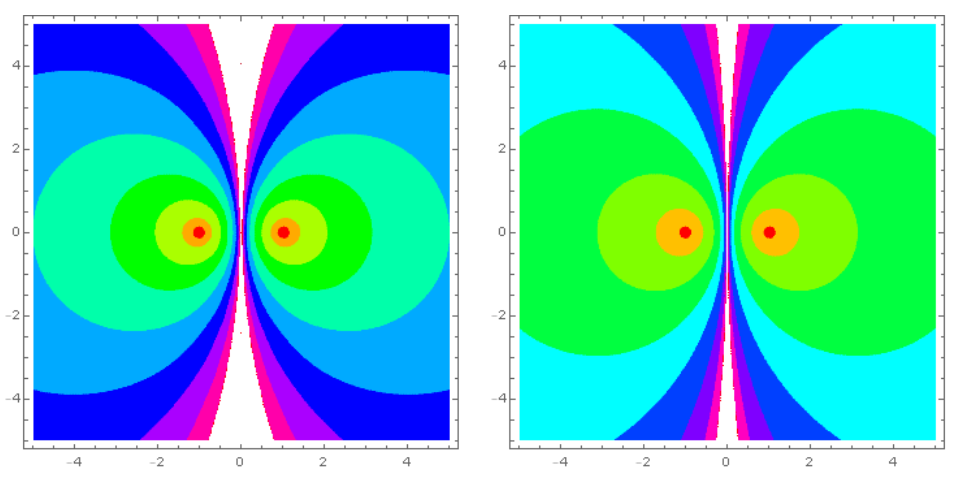
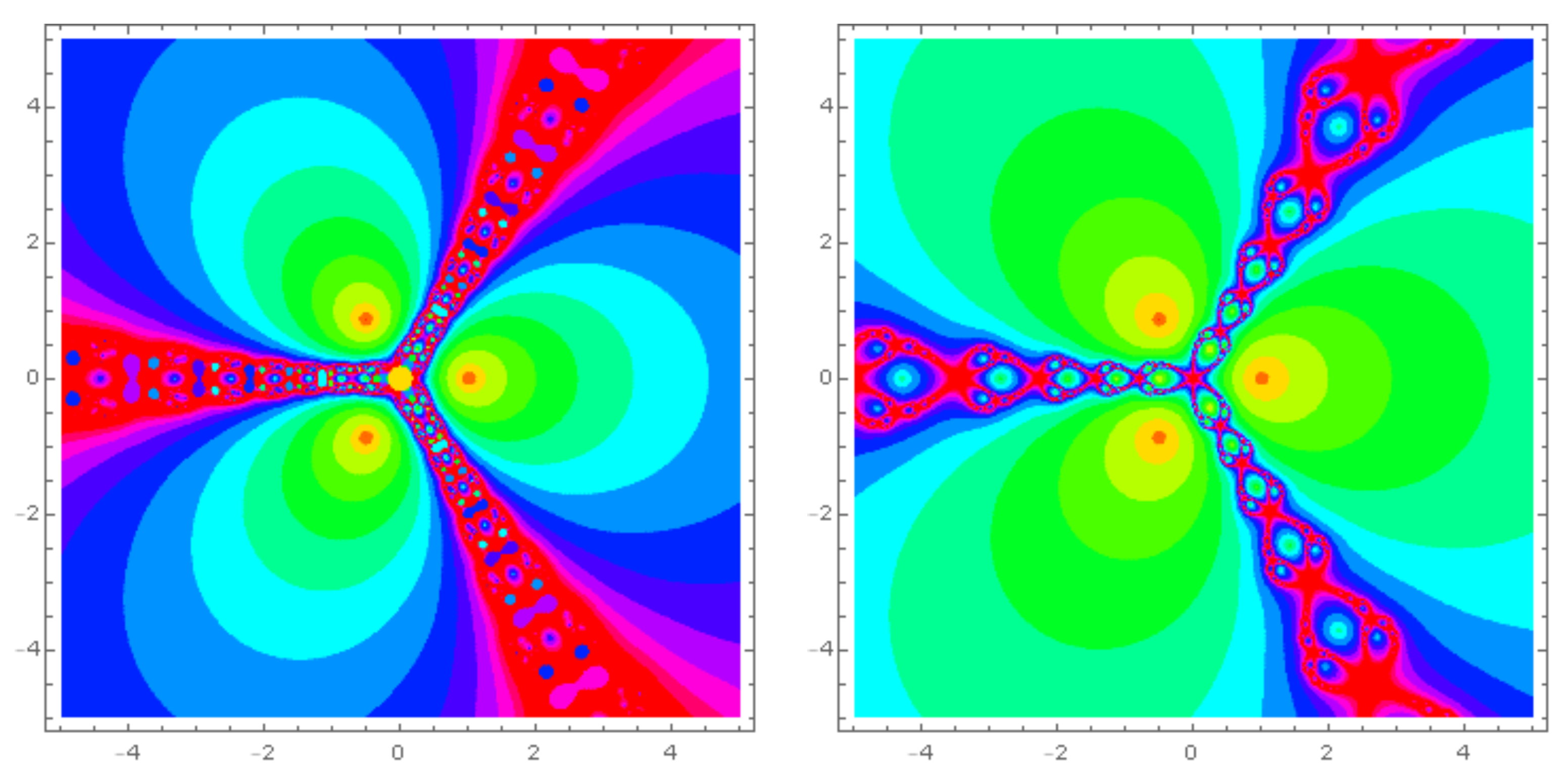
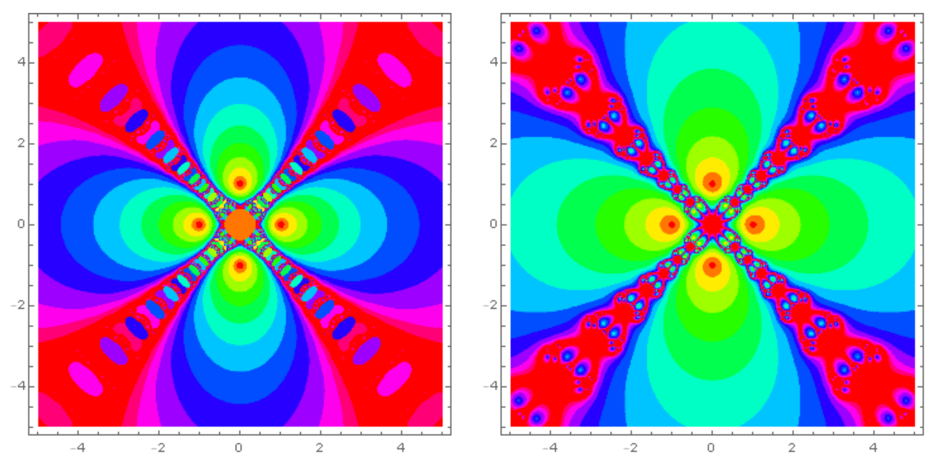
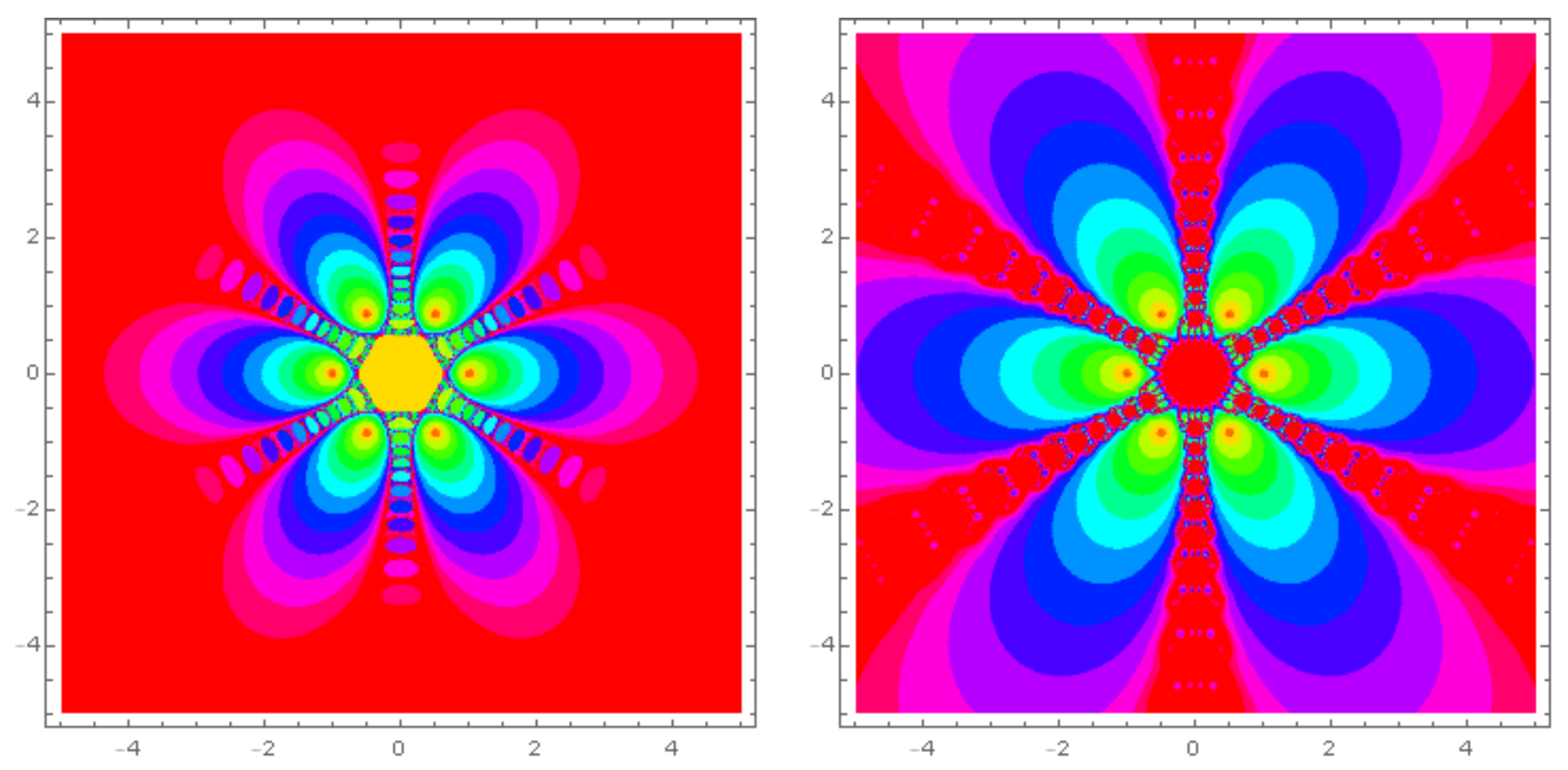
6]. Let us now draw the attraction basins of the methods (5) and (
2) in
Figure 1,
Figure 2,
Figure 3 and
Figure 4 for different polynomials in a square of the complex plane using double-precision arithmetic. Here, we follow the methodology discussed in [
7,
8] to find the attraction basins. Here, the red color stands for the risky area that could cause an indeterminate state or divergence. As can be observed clearly, the secant method has the lowest convergence rate and thus smaller converging areas, while this is improved for Newton’s method. Note that in this way,
initial approximations are tested one by one when we find the attraction basins.
The importance of the fractal behavior of different iterative schemes when applied to different polynomials is in the fact that they could reveal which method globally converges when it is extended for solving special matrix nonlinear equations. Important matrix functions that depend clearly on the attraction basins are matrix sign functions and sector functions.
This work focuses on finding and computing the matrix sign function, which plays a significant role in the theory and practical applications of the matrix function [
9].
The remaining portions of this paper are as follows. In
Section 2, a novel multi-step iteration method is proposed carefully to be employable for the calculation of the matrix sign.
Section 3 extends this method for calculating the sign of an invertible matrix. It is theoretically investigated how the solver converges and does this under asymptotical stability with an appropriate choice of the initial matrix. To test the efficacy and stability of the proposed solver, we examine numerical experiments on different test problems in
Section 4. Ultimately, based on the obtained computational observations, the suggested technique is determined to be efficient. The conclusion, with some outlines for the forthcoming works, is furnished in
Section 5.
2. Iteration Methods on the Sign of a Matrix
Let
be a nonsingular square matrix, and
g stands for a scalar function. The function
is defined as a matrix function of
A with the size
. If the function
g is given on the spectrum of the
A [
10,
11], then it is possible to have the facts below about the matrix function
:
For a given square matrix Z, it commutes with as long as Z commutes with A,
stand for the eigenvalues of , where are the eigenvalues of A,
,
,
commutes with A.
The sign of a matrix could be defined using the Cauchy integral as follows:
Some of the functions of matrices under given assumptions can be computed numerically by employing the fixed-point type iterative methods of the general form below:
wherein
must be chosen carefully.
The second-order Newton’s scheme has the following structure for calculating the sign of a square invertible matrix:
where the starting matrix is
The work [
12] presented an important family of iterative schemes for finding (
3) by employing the following Padé approximants:
Let us consider that the
-Padé approximate to
is defined by
and
. Then, the authors [
12] showed that the following iterative scheme
converges with convergence speed
to
.
By considering (
9), the following well-known locally convergent inversion-free Newton–Schulz method:
and the following Halley’s iteration scheme:
belong to this family for appropriate choices of
and
. It is noted that the Newton’s scheme (5) is a member of the reciprocal of (
9), see [
13,
14].
Two fourth-order methods from (
9) having global convergence behavior are given by
After discussing the existing iteration methods to find the matrix sign functions, this paper proposes a new one. It is known that the most challenging methods for such a purpose arises from (
9) with arbitrary order of convergence. Such methods are called optimal. However, in this paper, we present a novel root solver with global fourth-rate speed for our target to calculate the sign of a matrix.
A New Solver
The following nonlinear equation plays an important role when the solvers for the sign of a matrix are constructed (see e.g., [
15]):
The main aim here is to propose a new solver to be effective when it is extended for finding the matrix sign function. This means that when we now want to propose a new root solver, the purpose is not to fulfill the optimality conjecture of Kung–Traub for producing optimal root solvers or to design methods with memory to achieve as high an order of convergence as possible [
16]. In fact, the iterative root solver should be useful and new when it is applied to finding the matrix sign function. Therefore, many of the recent super-high-order methods are put aside. Here, we propose a three-step method without memory for such a target as follows:
It is necessary to show the convergence order of (
15) before any extensions to the matrix environments. This is pursued in the following theorem.
Theorem 1. Assume that is a simple root of the sufficiently differentiable function , and assume that the initial value is close to the solution. The scheme (15) has quartical convalescence rate and reads the error below:where and . Proof. Considering the assumption of the theorem, now we expand
and
around
to obtain that:
and
Now, from (
17) and (
18), we have
By substituting (
19) into
of (
15), we obtain
From (
17) and (
19), and a similar methodology, we obtain
Now, the use of (
15) and (
21) implies that
At last, by employing (
15) and (
22), it is possible to attain (
16). Therefore, the iteration (
15) has fourth-order convergence. □
Here, it might be asked how the scheme (
15) is built. Although the scheme is presented as a given, the presence of a detailed argument regarding the choice of such a scheme could make it possible to understand whether the scheme is unique or hides a class of possible schemes behind it. The scheme (
15) consists of three steps. The first two steps have been designed based on a Traub-like third-order method with the coefficients set to 9/30 and 39/30 to obtain the third order of convergence and as high a number as possible of the attraction basins. The last substep is based on the secant solver from the first and second steps, which includes the computation of a divided difference operator. To discuss further, this structure was obtained by us after severe attempts in order to fulfil the following:
3. A New Solver and Its Convergence
Let us now solve (
14) by the iterative method (
15). This can be symbolically deduced to the following numerical method in the matrix environment:
using the initial value (
6). Note that, similarly, one may obtain the reciprocal version of (
23) as follows:
Theorem 2. For computing the sign of A with no eigenvalues on the axis of imaginary, let be selected via (6). The iterative method (24) (or (23)) converges to the M, and the convergence order is four. Proof. We consider that
W is the Jordan block matrix,
K is an invertible matrix of the same size, and
A is decomposed by:
Now, by using the solver (
24) from the iterate
l to
, we obtain an iteration that maps the eigenvalues as follows (see [
14] for more information):
where
In general, and after some mathematical simplifications, the expression (
26) reveals that the eigenvalues conerge to
; that is to say,
The relation (
27) gives the convergence of the iteration to
via (
24). Now, to investigate the rate of convergence, we first write as follows:
Using (
28), we can write:
Using (
29), it is possible to obtain that:
which shows the fourth order of convergence. This completes the proof. The error analysis for (
23) can be deduced similarly. □
For economic reasons, it is important to employ an algorithm to solve practical problems. That is to say, the convergence rate is not the only factor, and a method is useful only if it can compete the most efficient existing solvers of the same type. When we compare (
24) to (
12) and (
13), it is observed that all possess four matrix products and only one matrix inversion per cycle. Moreover, it is now seen and checked that the proposed methods (
23) and (
24) have wider convergence radii.
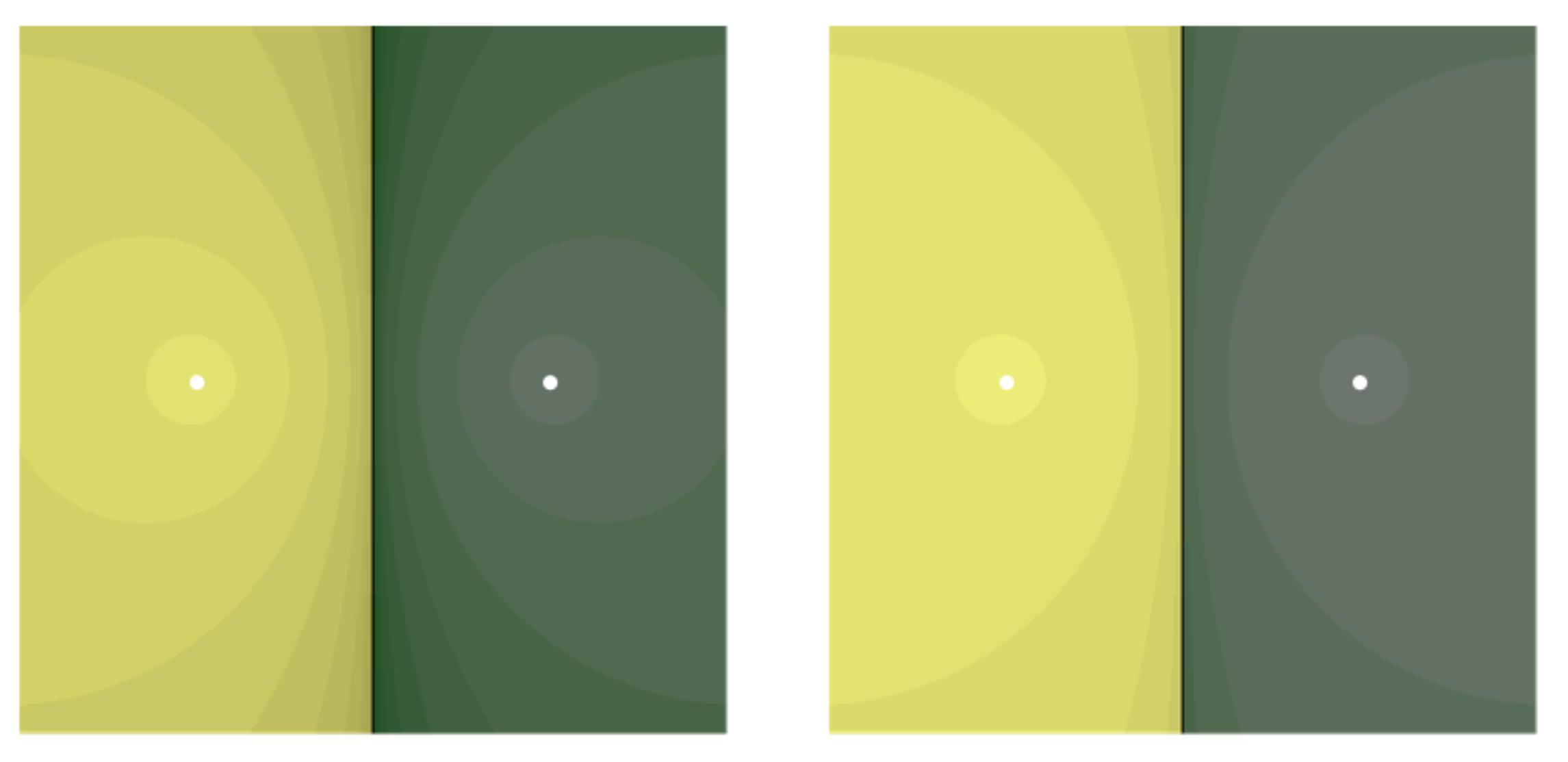
To check the global convergence of the presented method in contrast to the existing solvers, we may draw attraction basins of the iterative methods when solving (
14) on the complex domain
. In fact, we divide the domain into a refined mesh and test to what root each of the mesh points converge. The results of the comparisons are brought forward in
Figure 5 and
Figure 6 by employing the stopping termination
The results are shaded via the number of cycles required to attain the convergence. They also show that for (
23) and (
24), there are wider convergence radii, in contrast to their competitors of the same order from (
9).
Theorem 3. Using (24) and similar assumptions on A as in Theorem 2, then with is stable asymptotically. Proof. Let
stand for a computational perturbation that is produced in the
iterate. Now, one can write
From now on, it is also considered that
, which is via the first-order analysis of error in this theorem. This is valid if
is sufficiently small. Now, we obtain
For sufficiently large
l, that is to say, in the convergence phase, we consider that
where a note is used for simplifying
for any the matrix
U and any invertible matrix
L, and while we also use
, and
, in order to obtain the following relation:
By further simplifications and using
, we can find:
This can lead to the point that the method at the stage
is bounded, i.e., we have:
The inequality (
37) reveals that the sequence of matrices obtained by (
23) has asymptotical stability. This finishes the proof here. □
4. Numerical Treatments
In this section, the iterative solvers discussed up to now have been compared in the Mathematica 12.0 [
17] in
norm and the following termination:
The methods that will be compared are (5), (
11)–(
13), (
23), and (
24) (shown by Newton, Halley, Padé 4-1, Padé 4-2, PM1, and PM2, respectively). Other matrix norms might be employed in (
38). Although they might be very useful in terms of reducing the whole elapsed time for the compared methods, for the general case of complex dense matrices, the
would be a reliable choice. The stopping termination (
38) comes from the fact that at each iterate, the numerical approximation must satisfy the matrix nonlinear quadraric equation.
Example 1. We have tested all of the numerical methods of the same type on 10 randomly generated complex matrices given by the piece of Mathematica code below:
SeedRandom[456];
min = 11; number = 20;
Table[A[l] = RandomComplex[{-200 - 200 I,
200 + 200 I}, {50 l, 50 l}]; {l, min, number}];
tolerance = 10^−5;
The sizes are varied and are .
Results are provided in
Table 1 and
Table 2 showing that PM1 has the best performance against its competitors. Note that the convergence of the solvers for the matrix sign function depends on the suitable selection of the initial matrices. It is seen the PM1 beats all of its competitors by converging to the sign as quickly as possible. The mean number of iterates required to achieve the convergence, as well as the mean of the CPU elapsed times, is lower for the proposed solvers.
Thee computational tests in
Section 4 have been performed to show the efficacy of the new iteration method (and its reciprocal) for a variety of complex matrices of different sizes. The mean of the CPU times for (
23) and (
24) performed better than the others.
Example 2. The target of this problem is to compare the solvers for 10 real, randomly generated matrices of different sizes, as follows:
SeedRandom[123];
min = 11; number = 20;
Table[A[l] = RandomReal[{-1000, 1000},
{50 l, 50 l}]; {l, min, number}];
tolerance = 10^−5;
The results are given in Table 3 and Table 4, which confirm the superiority of the proposed solver against the existing solvers in terms of the number of iterates as well as the elapsed CPU time. 5. Concluding Remarks
To calculate the sign of an invertible matrix is always a significant problem in the theory and application of functions of matrices in mathematics. Accordingly, it is important to design new methods for such a purpose. Toward this goal, in this paper, after discussing the importance of studying the fractal behavior of iteration methods for solving nonlinear equations on different polynomials, we have proposed a new solver. The proposed multiplication-rich fourth-order method was developed, and its stability was proved, in this paper. Computational tests were performed to check the efficacy of the proposed solver and confirm the theoretical discussions. The presented scheme in this work has global convergence for the matrix sign, but like the other similar methods of the same structure, its convergence for the matrix sector function is local. This makes it important to investigate how to choose a proper starting matrix to be in the convergence phase when it is employed for finding the matrix-sector functions. Such an investigation is under investigation in our team for future research works.


