


Fractional Transformation-Based Intelligent H-Infinity Controller of a Direct Current Servo Motor

 ,
,  ,
,  ,
,
Abstract
:1. Nomenclature, Introduction, and Objectives
1.1. Nomenclature
1.2. Introduction
1.3. Contributions and Plan of the Article
2. Mathematical Modelling
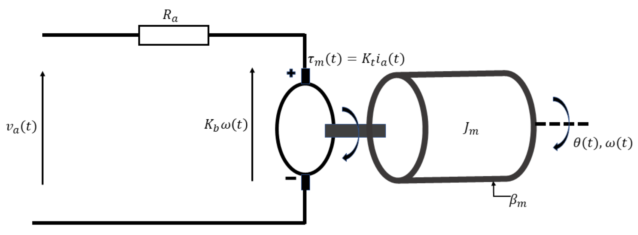
2.1. Description of the DC Servo Motor
2.2. Mathematical Model of the DC Servo Motor
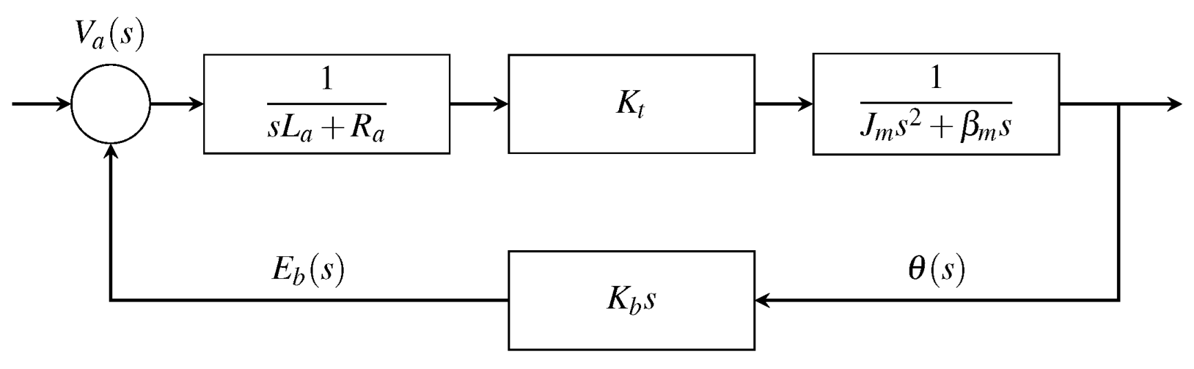
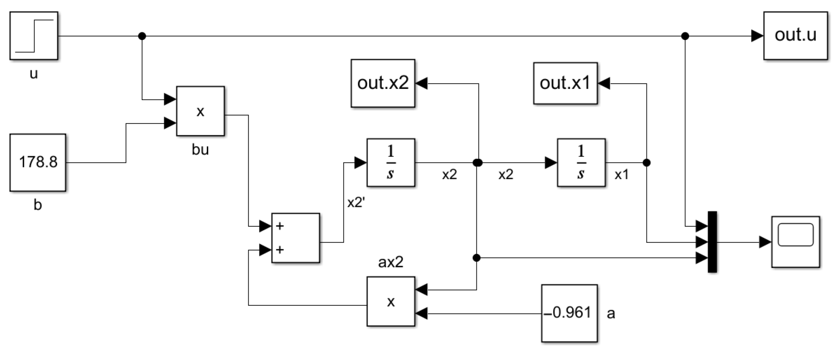
2.3. State-Space Model Equations of the DC Servo Motor
3. Design of Controllers for a DC Servo Motor System
3.1. PID Controller
3.2. Design of the Conventional H Controller
3.3. Design of the Proposed Intelligent Fixed-Structure H Controller
| Algorithm 1: Mayfly optimization approach |
 |
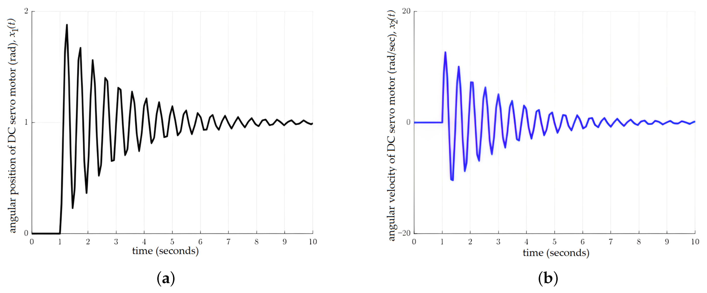
4. Comparison of Simulation Results for the Three Controllers
4.1. Setting
4.2. The Conventional Controllers
4.3. The Proposed Controller
5. Experimental Setup and Results
5.1. Experimental Setup for a DC Servo Motor
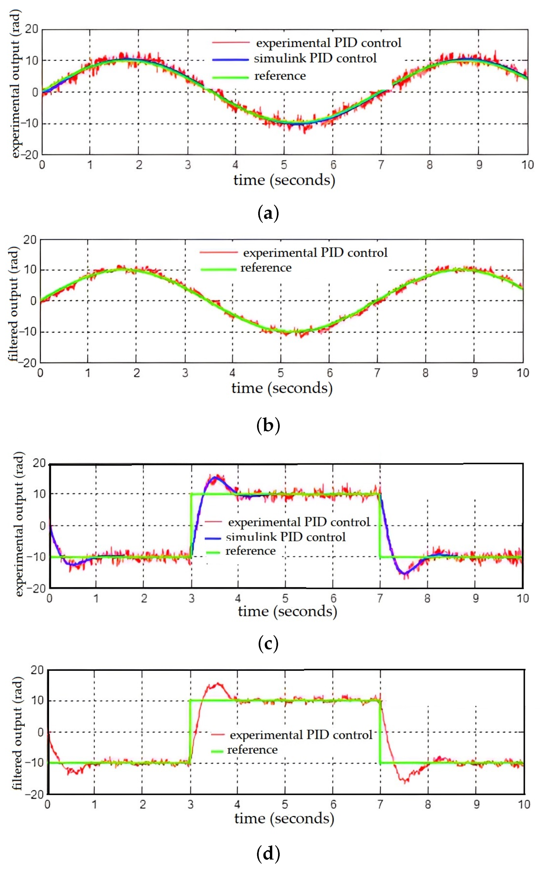
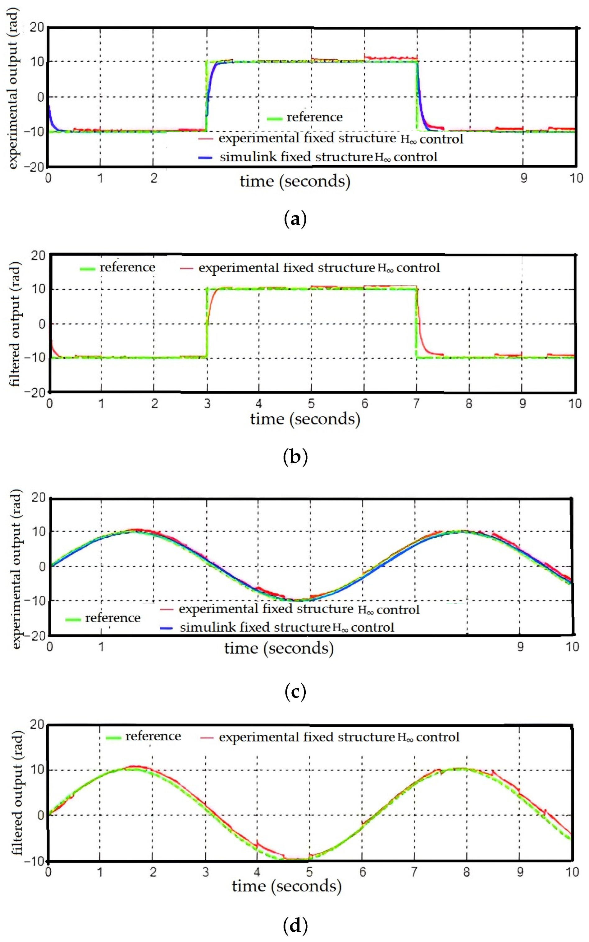
5.2. Results
6. Comparison, Discussion, and Conclusions
6.1. Performance Comparison and Discussion
6.2. Conclusions
Author Contributions
Funding
Institutional Review Board Statement
Informed Consent Statement
Data Availability Statement
Acknowledgments
Conflicts of Interest
References
- Wai, R.J.; Chen, P.C. Robust neural-fuzzy-network control for robot manipulator including actuator dynamics. IEEE Trans. Ind. Electron. 2006, 53, 1328–1349. [Google Scholar] [CrossRef]
- Low, K.S.; Chiun, K.Y.; Ling, K.V. Evaluating generalized predictive control for a brushless DC drive. IEEE Trans. Power Electron. 1998, 13, 1191–1198. [Google Scholar]
- Alshammari, O.; Kchaou, M.; Jerbi, H.; Aoun, S.B.; Leiva, V. A fuzzy design for a sliding mode observer-based control scheme of Takagi-Sugeno Markov jump systems under imperfect premise matching with bio-economic and industrial applications. Mathematics 2022, 10, 3309. [Google Scholar] [CrossRef]
- Wai, R.J.; Muthusamy, R. Fuzzy-neural-network inherited sliding-mode control for robot manipulator including actuator dynamics. IEEE Trans. Neural Netw. Learn. Syst. 2012, 24, 274–287. [Google Scholar]
- Dawson, D.M.; Hu, J.; Burg, T.C. Nonlinear Control of Electric Machinery; CRC Press: New York, NY, USA, 2019. [Google Scholar]
- Sevinc, A. A full adaptive observer for DC servo motors. Turk. J. Electr. Eng. Comput. Sci. 2003, 11, 117–130. [Google Scholar]
- Mehta, S.; Chiasson, J. Nonlinear control of a series DC motor: Theory and experiment. IEEE Trans. Ind. Electron. 1998, 45, 134–141. [Google Scholar] [CrossRef] [Green Version]
- Antić, D.; Milojković, M.; Jovanović, Z.; Nikolić, S. Optimal design of the fuzzy sliding mode control for a DC servo drive. J. Mech. Eng. 2010, 56, 455–463. [Google Scholar]
- Sharkawy, A.B.; Salman, S.A. An adaptive fuzzy sliding mode control scheme for robotic systems. Intell. Control Autom. 2011, 2, 299–309. [Google Scholar] [CrossRef] [Green Version]
- Charfeddine, S.; Alharbi, H.; Jerbi, H.; Kchaou, M.; Abbassi, R.; Leiva, V. A stochastic optimization algorithm to enhance controllers of photovoltaic systems. Mathematics 2022, 10, 2128. [Google Scholar] [CrossRef]
- Akar, M.; Temiz, I. Motion controller design for the speed control of DC servo motor. Int. J. Appl. Math. Inform. 2007, 1, 131–137. [Google Scholar]
- Liu, F.; Zhang, X. Compound adaptive fuzzy synchronization controller design for uncertain fractional-order chaotic systems. Fractal Fract. 2022, 6, 652. [Google Scholar] [CrossRef]
- Ackermann, J.; Guldner, J.; Sienel, W.; Steinhauser, R.; Utkin, V.I. Linear and nonlinear controller design for robust automatic steering. IEEE Trans. Control Syst. Technol. 1995, 3, 132–143. [Google Scholar] [CrossRef]
- Valluru, S.K.; Singh, M. Performance investigations of APSO tuned linear and nonlinear PID controllers for a nonlinear dynamical system. J. Electr. Syst. Inf. Technol. 2018, 5, 442–452. [Google Scholar] [CrossRef]
- Dubey, S.; Srivastava, S.K. A PID controlled real time analysis of DC motor. Int. J. Innov. Res. Comput. Commun. Eng. 2013, 1, 1965–1973. [Google Scholar]
- Mpanza, L.J.; Pedro, J.O. Optimised tuning of a PID-Based flight controller for a medium-scale rotorcraft. Algorithms 2021, 14, 178. [Google Scholar] [CrossRef]
- Sabir, M.M.; Khan, J.A. Optimal design of PID controller for the speed control of DC motor by using metaheuristic techniques. Adv. Artif. Neural Syst. 2014, 2014, 126317. [Google Scholar] [CrossRef]
- Muresan, C.I.; Birs, I.; Ionescu, C.; Dulf, E.H.; De Keyser, R. A review of recent developments in autotuning methods for fractional-order controllers. Fractal Fract. 2022, 6, 37. [Google Scholar] [CrossRef]
- Lien, C.H.; Chang, H.C.; Yu, K.W.; Li, H.C.; Hou, Y.Y. Robust H∞ controller design of switched delay systems with linear fractional perturbations by synchronous switching of rule and sampling input. Fractal Fract. 2022, 6, 479. [Google Scholar] [CrossRef]
- Doyle, J.; Glover, K.; Khargonekar, P.; Francis, B. State-space solutions to standard H2 and H∞ control problems. In Proceedings of the 1988 American Control Conference, Atlanta, GA, USA, 15–17 June 1988; pp. 1691–1696. [Google Scholar]
- Stein, G.; Doyle, J.C. Beyond singular values and loop shapes. J. Guid. Control Dyn. 1991, 14, 5–16. [Google Scholar] [CrossRef] [Green Version]
- McFarlane, D.; Glover, K. A loop-shaping design procedure using H/sub infinity/synthesis. IEEE Trans. Autom. Control 1992, 37, 759–769. [Google Scholar] [CrossRef]
- Rahman, M.Z.U.; Liaquat, R.; Rizwan, M.; Martin-Barreiro, C.; Leiva, V. A robust controller of a reactor electromicrobial system based on a structured fractional transformation for renewable energy. Fractal Fract. 2022, 6, 736. [Google Scholar] [CrossRef]
- Khalil, I.S.; Doyle, J.C.; Glover, K. Robust and Optimal Control; Prentice Hall: New York, NY, USA, 1996. [Google Scholar]
- Gahinet, P.; Apkarian, P. Decentralized and fixed-structure H∞ control in MATLAB. In Proceedings of the 50th IEEE Conference on Decision and Control and European Control Conference, Orlando, FL, USA, 12–15 December 2011; pp. 8205–8210. [Google Scholar]
- Diab, A.A.Z.; Al-Sayed, A.H.M.; Abbas Mohammed, H.H.; Mohammed, Y.S. Robust speed controller design using H∞ theory for high performance sensorless induction motor drives. In Development of Adaptive Speed Observers for Induction Machine System Stabilization; Springer: Singapore, 2019. [Google Scholar]
- Brezina, L.; Brezina, T. H-infinity controller design for a DC motor model with uncertain parameters. Eng. Mech. 2011, 18, 271–279. [Google Scholar]
- Dey, N.; Mondal, U.; Mondal, D. Design of a H-infinity robust controller for a DC servo motor system. In Proceedings of the 2016 International Conference on Intelligent Control Power and Instrumentation, Kolkata, India, 21–23 October 2016; pp. 27–31. [Google Scholar]
- Krishnan, T.D.; Krishnan, C.M.C.; Vittal, K.P. Design of robust H-infinity speed controller for high performance BLDC servo drive. In Proceedings of the 2017 International Conference on Smart grids, Power and Advanced Control Engineering, Bangalore, India, 17–19 August 2017; pp. 37–42. [Google Scholar]
- Apkarian, P.; Bompart, V.; Noll, D. Non-smooth structured control design with application to PID loop-shaping of a process. Int. J. Robust Nonlinear Control 2007, 17, 1320–1342. [Google Scholar] [CrossRef] [Green Version]
- Noll, D.; Apkarian, P.; Bompart, V. Nonsmooth structured control design. IFAC Proc. 2007, 40, 357–362. [Google Scholar] [CrossRef]
- Kaitwanidvilai, S.; Parnichkun, M. Genetic-algorithm-based fixed-structure robust h loop-shaping control of a pneumatic servo system. J. Robot. Mechatron. 2004, 16, 362–373. [Google Scholar] [CrossRef] [Green Version]
- Koch, G.G.; Osorio, C.R.; Pinheiro, H.; Oliveira, R.C.; Montagner, V.F. Design procedure combining linear matrix inequalities and genetic algorithm for robust control of grid-connected converters. IEEE Trans. Ind. Appl. 2019, 56, 1896–1906. [Google Scholar] [CrossRef]
- Schirrer, A.; Westermayer, C.; Hemedi, M.; Kozek, M. Robust H∞ control design parameter optimization via genetic algorithm for lateral control of a BWB type aircraft. IFAC Proc. 2010, 43, 57–63. [Google Scholar] [CrossRef]
- Ramirez-Figueroa, J.A.; Martin-Barreiro, C.; Nieto, A.B.; Leiva, V.; Galindo-Villardón, M.P. A new principal component analysis by particle swarm optimization with an environmental application for data science. Stoch. Environ. Res. Risk Assess. 2021, 35, 1969–1984. [Google Scholar] [CrossRef]
- Singh, V.P.; Mohanty, S.R.; Kishor, N.; Ray, P.K. Robust H-infinity load frequency control in hybrid distributed generation system. Int. J. Electr. Power Energy Syst. 2013, 46, 294–305. [Google Scholar] [CrossRef]
- Singh, V.P.; Kishor, N.; Samuel, P.; Mohanty, S.R. Impact of communication delay on frequency regulation in hybrid power system using optimized H-infinity controller. IETE J. Res. 2016, 62, 356–367. [Google Scholar] [CrossRef]
- Zhao, J.; Gao, Z.M. The fully informed mayfly optimization algorithm. In Proceedings of the 2020 International Conference on Big Data and Artificial Intelligence and Software Engineering, Chengdu, China, 23–25 October 2020; pp. 450–453. [Google Scholar]
- MatLab Team. Robust Control Toolbox 4.1; The Math Works, Inc.: Natick, MA, USA, 2011. [Google Scholar]
- Rahman, M.Z.U.; Shaikh, I.U.H.; Ali, A.; Ahmad, N. Fixed-structure Hα control of couple tank system and anti-integral windup PID control strategy for actuator saturation. In Proceedings of the 2016 World Congress on Industrial Control Systems Security, London, UK, 12–14 December 2016; pp. 1–6. [Google Scholar]
- Mehta, V.K.; Mehta, R. Principles of Electrical Machines; Chand Publishing: New Delhi, India, 2008. [Google Scholar]
- Inteco. Manual. In Modular Servo System (MSS). User’s Manual; Inteco: Krakow, Poland, 2006. [Google Scholar]
- Borase, R.P.; Maghade, D.K.; Sondkar, S.Y.; Pawar, S.N. A review of PID control, tuning methods and applications. Int. J. Dyn. Control 2021, 9, 818–827. [Google Scholar] [CrossRef]
- Shi, T.; Su, H.; Chu, J. Reliable H-infinity filtering for linear systems with sensor saturation. J. Control Theory Appl. 2013, 11, 80–85. [Google Scholar] [CrossRef]
- Gahinet, P.; Apkarian, P. Structured H∞ synthesis in MATLAB. IFAC Proc. 2011, 44, 1435–1440. [Google Scholar] [CrossRef]


| Abbreviation/Acronym | Definition |
|---|---|
| AC | Alternating current |
| A/D | Analog to digital |
| D/A | Digital to analog |
| DC | Direct current |
| EMF | Electromotive force |
| GA | Genetic algorithm |
| H | Hardy space of matrix-value functions |
| I/O | Input to output |
| LFT | Linear fractional transformation |
| LTI | Linear time invariant |
| MIMO | Multi-input multi-output |
| MSS | Modular servo system |
| PCI | Peripheral component interconnect |
| PID | Proportional integral derivative |
| PSO | Particle swarm optimization |
| PWM | Pulse-width modulation |
| Reference input | |
| RCT | Robust control toolbox |
| Sensitivity | |
| SIMO | Single-input multi-output |
| SISO | Single-input single-output |
| Complementary sensitivity |
| Contribution | Description |
|---|---|
| 1 | While considering the cost and complexity issues of conventional robust H controllers, we design a decentralized and fixed-structure robust control system [40]. Thus, the proposed intelligent fixed-structure H controller overcomes the hardware cost and complexity limitations. |
| 2 | The fixed-structure H controller has not been investigated for precisely tracking the position of the DC servo motor. |
| 3 | The proposed controller is robust and linear with a fixed structure and fixed order. |
| 4 | Intelligent optimization of tunable parameters with one degree of freedom for the fixed-structure robust H control problem is another contribution to the proposed research. For this purpose, the proposed fixed-structure H for the control problem is formulated in MATLAB with the help of the robust control toolbox [39]. |
| 5 | The proposed intelligent linear robust controller is also investigated on a real-time model of a DC servo motor. The performance of the proposed controller is compared with PID and conventional H controllers in terms of transient specifications, such as rise time, settling time, steady-state error, overshoot, and peak time. |
| Method | Description |
|---|---|
| Armature control | The angular velocity or position of the DC motor is controlled by varying the armature resistance. |
| Flux control | The flux variation is controlled by adding the resistance parallel to the armature of the DC motor. |
| Input voltage control | The input voltage to the armature of the DC servo motor is varied to control the angular velocity or position of the shaft. |
| Variable | Description |
|---|---|
| Input voltage. | |
| Armature current. | |
| Angular position. | |
| Angular velocity. | |
| Armature resistance. | |
| Inertia moment. | |
| Damping coefficient. | |
| Back EMF. | |
| Electromechanical torque. |
| Variable | Description |
|---|---|
| Angle in radians (rad), which determines the angular shaft position. | |
| Velocity in rad/sec, which represents the angular shaft velocity. |
| Symbol | Values | Units |
|---|---|---|
| 12.00 | V | |
| 1.04 | sec | |
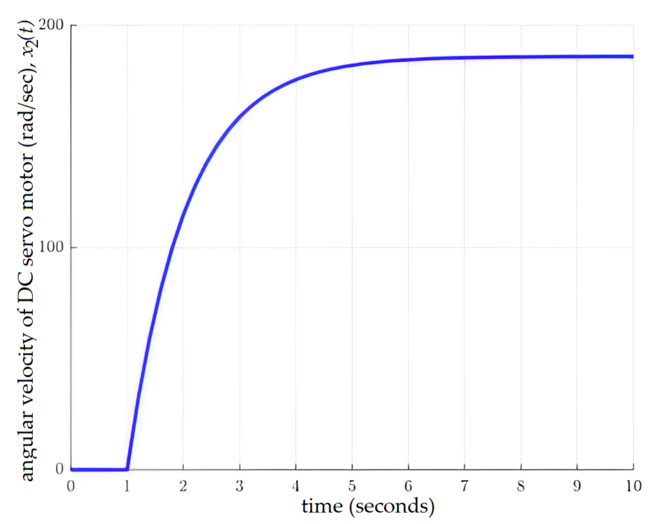
| 186.00 | rad/sec | |
| a | −0.96 | seg |
| b | 178.80 | rad/seg |
| Symbol | Description | Value |
|---|---|---|
| Proportional gain | 0.1405 | |
| Integral gain | 0.0305 | |
| Derivative gain | 0.0240 |
| Symbol | Description | Value |
|---|---|---|
| Proportional gain | 0.0806 | |
| Integral gain | ||
| Derivative gain | 0.086 | |
| 1st order differential coefficient | 0.000129 |
| Controller | Controller | Rise Time | Settling Time | Over-Shoot | Steady-State |
|---|---|---|---|---|---|
| Order | (sec) | (sec) | (%) | Error | |
| Traditional PID | 0.25 | 2.5 | 24.2 | 0% | |
| Conventional H | 3rd | 0.20 | 0.35 | 0 | 0% |
| Intelligent fixed-structure H | 2nd | 0.18 | 0.33 | 0 | 0% |
| Module | Description |
|---|---|
| Tacho generator | Converter of mechanical energy into electrical energy. A tacho generator measures the angular shaft speed and provides output in the form of voltage proportional to the angular velocity. |
| Encoder | Measurer of the angular rotation of the DC motor. The potentiometer is connected outside the servo mechanism. |
| MSS | Connecter of backlash, magnetic brake, gearbox, and circular disk using the MSS inertia load in the chain. |
| MSS toolbox | Tool operated directly in the Simulink of MATLAB environment. This MSS toolbox has the excess of all the PCI/RTDAC acquisition board functions. The PCI board is equipped with an A/D converter, and the whole measurement system is based on this PCI board equipped with an A/D converter. |
| PCI board | Controller of angular speed and position of the DC motor. The PWM pulses are generated in an appropriate sequence. The DC motor is configured with PCI board and I/O board for communication purposes. The PCI board reads encoder signals and produces PWM pulses in the appropriate sequence to control the servo motor. |
Disclaimer/Publisher’s Note: The statements, opinions and data contained in all publications are solely those of the individual author(s) and contributor(s) and not of MDPI and/or the editor(s). MDPI and/or the editor(s) disclaim responsibility for any injury to people or property resulting from any ideas, methods, instructions or products referred to in the content. |
© 2022 by the authors. Licensee MDPI, Basel, Switzerland. This article is an open access article distributed under the terms and conditions of the Creative Commons Attribution (CC BY) license (https://creativecommons.org/licenses/by/4.0/).
Share and Cite
Rahman, M.Z.U.; Leiva, V.; Martin-Barreiro, C.; Mahmood, I.; Usman, M.; Rizwan, M. Fractional Transformation-Based Intelligent H-Infinity Controller of a Direct Current Servo Motor. Fractal Fract. 2023, 7, 29. https://doi.org/10.3390/fractalfract7010029
Rahman MZU, Leiva V, Martin-Barreiro C, Mahmood I, Usman M, Rizwan M. Fractional Transformation-Based Intelligent H-Infinity Controller of a Direct Current Servo Motor. Fractal and Fractional. 2023; 7(1):29. https://doi.org/10.3390/fractalfract7010029
Chicago/Turabian StyleRahman, Muhammad Zia Ur, Víctor Leiva, Carlos Martin-Barreiro, Imran Mahmood, Muhammad Usman, and Mohsin Rizwan. 2023. "Fractional Transformation-Based Intelligent H-Infinity Controller of a Direct Current Servo Motor" Fractal and Fractional 7, no. 1: 29. https://doi.org/10.3390/fractalfract7010029