Article

A Cubic Spline Collocation Method to Solve a Nonlinear Space-Fractional Fisher’s Equation and Its Stability Examination

1
Department of Mathematics and Computer Science, Faculty of Science, Menoufia University, Shebin El-Kom 13829, Egypt
2
Department of Mathematics, Faculty of Science, Damanhour University, Damanhour 22511, Egypt
3
Department of Mathematics, College of Science and Arts in Ar-Rass, Qassim University, Ar Rass 51452, Saudi Arabia
4
Department of Mathematics and Statistics, Faculty of Management Technology and Information Systems, Port Said University, Port Said 42511, Egypt
*
Author to whom correspondence should be addressed.
Fractal Fract. 2022, 6(9), 470; https://doi.org/10.3390/fractalfract6090470
Submission received: 20 July 2022 / Revised: 19 August 2022 / Accepted: 22 August 2022 / Published: 26 August 2022
(This article belongs to the Special Issue Advances in Fractional Differential Operators and Their Applications)

Abstract

:
This article seeks to show a general framework of the cubic polynomial spline functions for developing a computational technique to solve the space-fractional Fisher’s equation. The presented approach is demonstrated to be conditionally stable using the von Neumann technique. A numerical illustration is given to demonstrate the proposed algorithm’s effectiveness. The novelty of the present work lies in the fact that the results suggest that the presented technique is accurate and convenient in solving such problems.

1. Introduction

Fractional calculus is a generalization of classical calculus that deals with fractional order differentiation and integration operations. Everyone who has studied elementary calculus is familiar with the differentiation operator, D = d / d x . Additionally, the n th derivative of a suitable function, D n f ( x ) = d n f ( x ) / d n x , is properly defined as long as n is a positive integer. In 1695, L’Hopital enquired to Leibniz about the meaning of D n f if n was fractional. Many prominent mathematicians, including Euler, Laplace, Fourier, Abel, Liouville, Riemann, and Laurent, have since studied time-fractional calculus. However, it was not until 1884 that the theory of generalized operators progressed to the point where it could be used as a starting point for modern mathematicians. Fractional calculus has been utilized in thermodynamics, viscoelasticity, bioengineering, aerodynamics, control theory, electromagnetics, finance, chemistry, and signal processing in recent decades [1,2,3]. Fractional calculus theory dates back to Leibniz in the sixteenth century, and many different types of fractional operators have been created and developed virtually as far as the classical theory has evolved. The Riemann–Liouville, Caputo, conformable, and Riesz operator approaches are among these [4,5,6,7,8,9]. Fractional differential equations (FDEs) appear in engineering processes, a number of physical phenomena, financial products, and biological systems, such as non-exponential relaxation patterns and anomalous diffusion [10]. Several numerical methods have been developed to obtain an approximate solution of FDEs. These methods include the Adomian decomposition method [11], finite difference method [12], variational iteration method [13], spectral methods [14], and homotopy perturbation method [15,16].
Fisher [17] introduced the nonlinear fractional Fisher equation as a mathematical model to describe the kinetic advancing rate of an advantageous gene. The fractional Fisher’s equation is also used in autocatalytic chemical reactions, nuclear reactor theory, neurophysiology, flame propagation, and branching Brownian motion processes [18,19,20]. In the open literature, many works describe solving the nonlinear fractional Fisher equation, see [20,21,22,23]. In our article, we propose a cubic polynomial spline-based technique for obtaining approximation solutions for the space-fractional Fisher’s equation in the following form [24]:
α u ( x ,   t ) x α = u ( x ,   t ) t u ( x ,   t ) ( 1 u ( x ,   t ) ) + f ( x ,   t ) ,   x > 0 ,
subject to the conditions:
u ( a ,   t ) = 1 ( t ) ,   u ( b ,   t ) = 2 ( t ) ,   0 < t T ,  
and
u ( x ,   0 ) = g ( x ) ,   a x b ,
where α is a parameter in the Caputo sense that describes the fractional order of the space derivative, and 1 < α 2 ; if we take α = 2 , Equation (1) reduces to the classical nonlinear Fisher’s equation. Several scholars have studied and solved the space-fractional nonlinear Fisher’s equation using various numerical techniques, for example, the generalized differential transform method (GDTM) and the variational iteration method (VIM) [25], the radial basis functions method [26], the quadratic polynomial spline-based method (QPSM) [24], and the Legendre spectral collocation method [27]. The above-mentioned articles show how to solve the space-fractional Fisher’s equation in which the exact solution is unknown, but, as far as we are aware, no papers are using cubic polynomial spline for space-fractional Fisher’s equation; hence, that is the motivation for our study.
Definition 1.
The Caputo space-fractional derivative operator of order α > 0 is given by [25]:
D x α a C u ( x ,   t ) = α u ( x ,   t ) x α = { 1 Γ ( n α ) a x n u ( τ ,   t ) τ n ( x τ ) n α 1 d τ ,                                     n 1 < α < n , n u ( x ,   t ) x n ,                                                                                                                                         α = n ,  
where Γ (   ) is the gamma function. The right and left Caputo fractional derivatives of order α are given, respectively, by [28]:
D x C b α u ( x ,   t ) = 1 Γ ( n α ) x b ( 1 ) n n u ( τ ,   t ) τ n ( τ x ) n α 1 d τ ,   n 1 < α n ,
D a C x α u ( x ,   t ) = 1 Γ ( n α ) a x n u ( τ ,   t ) τ n ( x τ ) n α 1 d τ ,   n 1 < α n .
The numerical solutions of fractional differential equations using numerical methods with spline functions and their use is an important area of research in numerical analysis, see [29,30,31,32,33,34]. Such problems appear very often in physics, engineering, medicine, biology, and other sciences. Spline functions can be integrated and differentiated due to being piecewise polynomials and, since they have a basis with small support, many of the integrals that occur in numerical methods are zero. Numerical methods with spline functions in obtaining the numerical solution of the differential equations lead to band matrices with a low computational cost. Cubic splines were used instead of using linear or quadratic splines, because they produce smooth approximations while maintaining a low computational cost.
Definition 2.
Polynomial Spline Function [35,36]:
Let a = x 0 < < x n 1 < x n = b be a subdivision of the interval [ a ,   b ] and m Ν . A function P :   [ a ,   b ] R is called a spline of degree m for this subdivision if P is ( m 1 ) times continuously differentiable on [ a ,   b ] and if the restriction of P to each subinterval [ x i ,   x i + 1 ] for i = 0 ,   1 ,   ,   n 1 reduces to a polynomial of degree at most m . Thus, the polynomial spline function has the form:
P ( x ) = { P 0 ( x ) ,   P 1 ( x ) ,       P n 1 ( x ) ,   if   x [ x 0 ,   x 1 ] , if   x [ x 1 ,   x 2 ] ,   if   x [ x n 1 ,   x n ] .
such that each polynomial spline segment is given by:
P i ( x ) = r = 0 m a i r ( x x r ) r ,   i = 0 ,   1 ,   ,   n 1 ,   x [ x i ,   x i + 1 ] .
The remainder of this article is structured as follows. In Section 2, a method is proposed that is based on the cubic spline polynomial method. In Section 3, the von Neumann method is used to discuss stability theoretically. In Section 4, we use a numerical example to demonstrate the suggested method’s efficiency and accuracy. The conclusion is presented in Section 5.

2. Derivation of the Method

To approximate u ( x ,   t ) by a cubic polynomial spline-based method over finite elements, let the region M = [ a ,   b ] × [ 0 ,   T ] be discretized by a set of points M i j , which are the vertices of a grid of points ( x i ,   t j ) where x i = a + i h , with h = Δ x = b a N for each i = 0 ,   1 ,   ,   N and t j = j k , k = Δ t for j = 0 ,   1 ,   ,   R .
Let W i j be an approximation to u ( x i ,   t j ) obtained by the segment P i ( x i ,   t j ) of the spline function passing through the points ( x i ,   W i j ) and ( x i + 1 ,   W i + 1 j ) . Each segment has the form [37,38]:
P i ( x ,   t j ) = a i ( t j )   ( x x i ) 3 + b i ( t j )   ( x x i ) 2 + c i ( t j )   ( x x i ) + d i ( t j ) ,
for each i = 0 ,   1 ,   ,   N 1 . To obtain expressions for the coefficients of Equation (4) in terms of W i j , W i + 1 j , S i j , and S i + 1 j , we first define:
P i ( x i ,   t j ) = W i j ,
P i ( x i + 1 ,   t j ) = W i + 1 j ,
P i ( α ) ( x i ,   t j ) = α x α P i ( x i ,   t j ) = S i j ,
P i ( α ) ( x i + 1 ,   t j ) = α x α P i ( x i + 1 ,   t j ) = S i + 1 j ,  
where 1 < α 2 . By using (4), (5), and (6), we have:
d i = W i j   ,
  h 3 a i + h 2 b i + h c i + d i = W i + 1 j ,
where a i a i ( t j ) ,   b i b i ( t j ) ,   c i c i ( t j ) , and d i d i ( t j ) . Using the right Caputo fractional derivative and (4) in (7), we obtain:
α x α P i ( x i ,   t j ) = 1 Γ ( 2 α ) x i x i + 1 ( τ x i ) 1 α P i ( 2 ) ( τ ,   t j ) d τ = 6 ( 2 α ) h 3 α Γ ( 4 α ) a i + 2 h 2 α Γ ( 3 α ) b i = S i j ,
and from using the left Caputo fractional derivative and (4) in (8), we obtain:
α x α P i ( x i + 1 ,   t j ) = 1 Γ ( 2 α ) x i x i + 1 ( x i + 1 τ ) 1 α P i ( 2 ) ( τ ,   t j ) d τ = 6 h 3 α Γ ( 4 α ) a i + 2 h 2 α Γ ( 3 α ) b i = S i + 1 j ,
We obtain the following expressions by solving (9)–(12):
a i = Γ ( 4 α ) 6 ( 1 α ) h 3 α ( S i j S i + 1 j ) ,
b i = Γ ( 3 α ) 2 ( 1 α ) h 2 α ( ( 2 α ) S i + 1 j S i j ) ,
c i = 1 h ( W i + 1 j W i j ) + Γ ( 4 α ) 6 ( 1 α ) h 1 α ( S i + 1 j S i j ) + Γ ( 3 α ) 2 ( 1 α ) h 1 α ( S i j ( 2 α ) S i + 1 j ) ,
d i = W i j .
Using the first derivative’s continuity condition at x = x i , that is P i ( 1 ) ( x i ,   t j ) = P i 1 ( 1 ) ( x i ,   t j ) , we obtain:
c i c i 1 = 3 h 2 a i 1 + 2 h b i 1
Substituting the expressions a i , b i   ,   and   c i from Equation (13) into Equation (14), we obtain:
W i + 1 j 2 W i j + W i 1 j + Γ ( 4 α ) 6 ( 1 α ) h α ( S i + 1 j S i j ) + Γ ( 3 α ) 2 ( 1 α ) h α ( S i j ( 2 α ) S i + 1 j ) + Γ ( 4 α ) 6 ( 1 α ) h α ( S i 1 j S i j ) + Γ ( 3 α ) 2 ( 1 α ) h α ( ( 2 α ) S i j S i 1 j ) = Γ ( 4 α ) 2 ( 1 α ) h α ( S i 1 j S i j ) + Γ ( 3 α ) ( 1 α ) h α ( ( 2 α ) S i j S i 1 j ) .  
Equation (15) can be rewritten in the form:
W i + 1 j 2 W i j + W i 1 j = ( Γ ( 4 α ) 2 ( 1 α ) h α Γ ( 3 α ) ( 1 α ) h α Γ ( 4 α ) 6 ( 1 α ) h α + Γ ( 3 α ) 2 ( 1 α ) h α ) S i 1 j + ( 2 Γ ( 4 α ) 6 ( 1 α ) h α Γ ( 3 α ) 2 ( 1 α ) h α ( 2 α ) Γ ( 3 α ) 2 ( 1 α ) h α Γ ( 4 α ) 2 ( 1 α ) h α + ( 2 α ) Γ ( 3 α ) ( 1 α ) h α ) S i j + ( ( 2 α ) Γ ( 3 α ) 2 ( 1 α ) h α Γ ( 4 α ) 6 ( 1 α ) h α ) S i + 1 j
After slight rearrangements, Equation (16) becomes:
W i 1 j 2 W i j + W i + 1 j = β S i 1 j + γ S i j + β S i + 1 j ,   i = 1 ,   ,   N 1 ,
where β = ( 2 α 3 ) h α Γ ( 3 α ) 6 ( α 1 ) and γ = α h α Γ ( 3 α ) 3 ( α 1 ) . As α 2 , system (17) reduces to:
W i 1 j 2 W i j + W i + 1 j = 1 6 ( S i 1 j + 4 S i j + S i + 1 j ) ,   i = 1 ,   ,   N 1 .
Remark 1:
For Equation (17), the local truncation error is:
T i * j = β ( u i 1 j + u i + 1 j ) 2 γ u i j β ( D x 2   u i 1 j + D x 2 u i + 1 j ) γ D x 2 u i j ,  
and can be obtained by expanding this equation in terms of u ( x i , t j ) and its derivatives in the Taylor series, as follows:
T i * j = ( h 2 ( γ + 2 β ) ) D x 2 u i j + ( h 4 12 β h 2 ) D x 4 u i j + ( h 6 360 β h 4 12 ) D x 6 u i j + .
Then, the last expression T i * j can be written as:
T i * j = h α ( h 2 - α θ ) D x 2 u i j + h 2 + α ( h 2 - α 12 δ ) D x 4 u i j + h 4 + α ( h 2 - α 360 δ 12 ) D x 6 u i j + .  
where θ = Γ ( 3 α ) and δ = ( 2 α 3 ) Γ ( 3 α ) 6 ( α 1 ) . From the expression (21) of the local truncation error, our scheme (17) is reduced to O ( h α ) , 1 < α 2 .
The fractional Fisher’s Equation (1) can now be defined as follows in terms of S i j :
S i j = α W i j x α = W i j t W i j ( 1 W i j ) + f ( x i ,   t j ) .
Using the finite difference method, we obtain:
W i j t W i j W i j 1 k .
This allows us to express S i 1 j , S i j , and S i + 1 j as follows:
S i 1 j = W i 1 j W i 1 j 1 k σ i 1 j W i 1 j + f i 1 j , S i j = W i j W i j 1 k σ i j W i j + f i j , S i + 1 j = W i + 1 j W i + 1 j 1 k σ i + 1 j W i + 1 j + f i + 1 j ,
where σ i j = ( 1 W i j ) . Substituting (22) into (17) gives us the following system:
A i W i 1 j + B i W i j + C i W i + 1 j = A i * W i 1 j 1 + B i * W i j + C i * W i + 1 j 1 + ρ i j   , i = 1 ,   ,   N 1 ,   j = 1 ,   ,   R ,
where:
A i = k β + β k σ i 1 j ,   A i * = β ,
B i = 2 k γ + γ k σ i j ,   B i * = γ ,
C i = k β + β k σ i + 1 j ,   C i * = β ,
and:
ρ i j = β k f i 1 j + γ k f i j + β k f i + 1 j .
System (23) consists of N 1 equations in the unknowns W i , i = 0 ,   1 ,   , N . Two additional equations are required to solve this system. The boundary conditions in (2) are used to derive these equations, which can be represented as:
W 0 j = 1 ( t j ) ,   W N j = 2 ( t j ) ,   j = 0 ,   1 ,   ,   R .  
Writing (23) and (24) in matrix form gives:
Φ W j = Φ * W j 1 + r j ,
where:
W j = ( W 0 j ,   W 1 j ,   W 2 j ,       ,   W N 1 j ,   W N j ) T ,
Φ = [ 1 0 0 0 0 0 0 A 1 B 1 C 1 0 0 0 0 0 A 2 B 2 C 2 0 0 0 0 0 0 0 A N 1 B N 1 C N 1 0 0 0 0 0 0 1 ] ,
Φ * = [ 0 0 0 0 0 0 0 A 1 * B 1 * C 1 * 0 0 0 0 0 A 2 * B 2 * C 2 * 0 0 0 0 0 0 0 A N 1 * B N 1 * C N 1 * 0 0 0 0 0 0 0 ] ,
and,
r j = ( 1 ( t j ) ,   ρ 1 j ,   ρ 2 j ,       ,   ρ N 1 j ,   2 ( t j ) ) T
where Φ * and Φ are ( N + 1 ) × ( N + 1 ) matrices and W j and r j are ( N + 1 ) vectors.
Now, the initial condition, u ( x ,   t 0 ) = g ( x ) for a x b , implies that W i 0 for i = 0 ,   1 ,   ,   N . These values can be utilized in (25) to obtain the value of W i 1 for i = 0 ,   1 ,   ,   N . If the technique is reapplied once all the approximations W i 1 are determined, the values of W i 2 , W i 3 , …, W i R can be derived in the same way.
The nonlinear term in the system is linearized using the technique in (25). For example, if j = 1 , we approximate σ i 1 by σ i 1 * computed from w i 0 , which obtains an approximation to w i 1 . For j = m , we approximate σ i m by σ i m * computed from w i m 1 and obtain an approximation to w i m .

3. Stability Analysis

The von Neumann technique will be used to investigate our system’s stability (23). To do this, we must linearize the nonlinear term u ( x ,   t ) ( 1 u ( x ,   t ) ) of Fisher’s Equation (1), by assuming that the corresponding quantities σ i 1 j , σ i j , and σ i + 1 j are equal to a local constant λ * in (23). The key part of the von Neumann analysis is to assume a solution of the form [39]:
W i j = ξ j exp ( φ q i h ) ,
where q = 1 , h is the element size, φ is the mode number, and ξ j is the amplification factor at time level j . As j increases (more time steps are computed), adding the latter W i j expression to the system (23) gives the following characteristic equation:
ξ j ( A i exp ( φ q ( i 1 ) h ) + B i exp ( φ q i h ) + C i exp ( φ q ( i + 1 ) h ) )   = ξ j 1 ( A i * exp ( φ q ( i 1 ) h ) + B i * exp ( φ q i h ) + C i * exp ( φ q ( i + 1 ) h ) ) ,
where:
A i = k β + β k λ * ,   A i * = β ,
B i = 2 k γ + γ k λ * , B i * = γ ,
C i = k β + β k λ * , C i * = β ,
After simple basic calculations, (27) becomes:
ξ = A i * exp ( q ϕ ) + B i * + C i * exp ( q ϕ ) A i exp ( q ϕ ) + B i + C i exp ( q ϕ ) ,
where ϕ = φ h . After using Euler’s formula exp ( q ϕ ) = cos ϕ + q   sin ϕ , the last equation (28) can be simplified as:
ξ = ( A i * + C i * ) cos ϕ + B i * + q ( C i * A i * ) sin ϕ ( A i + C i ) cos ϕ + B i + q ( C i A i ) sin ϕ .
Equation (29) can be rewritten in the forms:
ξ = 2 β cos ϕ γ ( 2 k 2 β + 2 β k λ * ) cos ϕ + ( 2 k γ + γ k λ * ) .  
or
ξ = ( 2 β cos ϕ + γ ) ( 2 β cos ϕ + γ ) + 2 k ( 1 cos ϕ ) λ * ( 2 β k cos ϕ + γ k ) .  
The quantity ( 1 cos ϕ ) is positive or equal to zero but 2 β cos ϕ + γ is surely positive if we choose γ > 0 and β > 0 such that γ > 2 β . If we choose k , β , and γ small enough to make λ * ( 2 β k cos ( ϕ ) + γ k ) 0 , then last (31) is close to:
ξ = ( 2 β cos ϕ + γ ) ( 2 β cos ϕ + γ ) + 2 k ( 1 cos ϕ ) .  
For stability, we must have | ξ | 1 (otherwise ξ j in (26) would expand in an unbounded manner). This condition is satisfied for γ > 0 and β > 0 such that γ > 2 β . Finally, we can say that our numerical scheme is conditionally stable for γ > 0 , β > 0 , and γ > 2 β , if k , β , and γ values chosen are small enough.

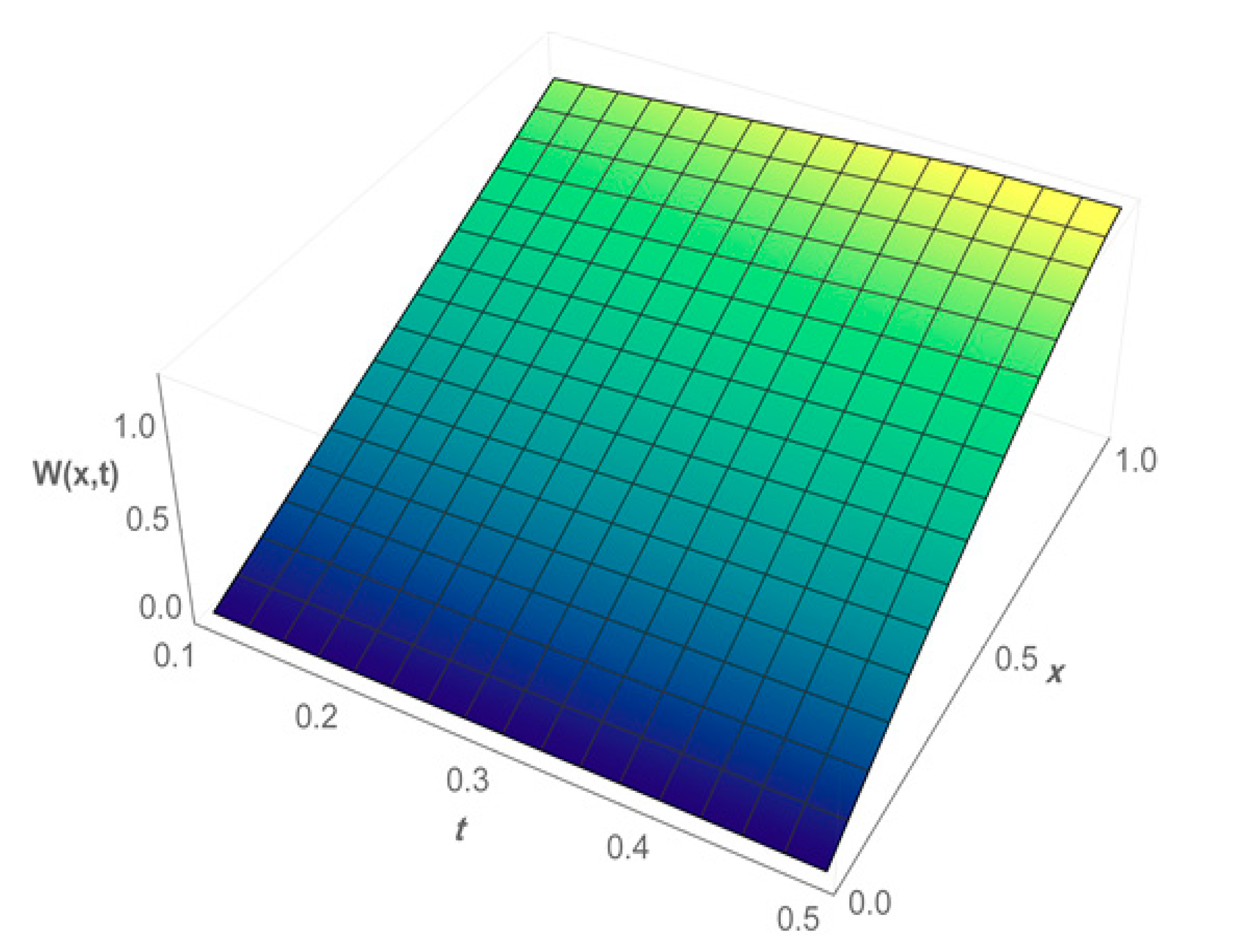
4. Numerical Results

In this part, we employ the suggested method for solving the nonlinear space-fractional Fisher’s equation [17,18] with α = 1 . 5 , f ( x ,   t ) = x 2 , and u ( x ,   0 ) = x and subject to conditions:
u ( 0.0125 ,   t ) 0.0125 ( 1 + t ) + 0.00609375 t 2 0.082176 t 3 0.0210541 t 4 7.16634 × 10 6   t 5 ,
u ( 1.0125 ,   t ) 1.0125 ( 1 + t ) 0.518906 t 2 0.921366   t 3 + 0.310529 t 4 + 0.0845434   t 5 .
The solution of the space-fractional Fisher’s equation, like that of most fractional partial differential equations, is unknown, so we will compare it with the known computational approaches such as GDTM and VIM. We used k = 0.0005 and N = 80 in all our numerical results. Table 1, Table 2 and Table 3 compare our method, which was improved in Section 2, to other existing methods.
Table 1, Table 2 and Table 3 show that for all values of x and t , our approximate solutions are in good agreement with the approximate solutions using other existing methods. This is also shown in Figure 1 and Figure 2.

5. Conclusions

The nonlinear space-fractional Fisher’s equation is numerically treated in this article using a collocation method with cubic polynomial spline functions. The proposed method is demonstrated to be conditionally stable using the von Neumann stability technique. Compared to other useful techniques, such as VIM, GDTM, and QPSM, the numerical results illustrate that our proposed method retains efficiency, capability, and good versatility. The findings of our study are hoped to pique the attention of academics interested in using the cubic polynomial spline to numerically solve nonlinear fractional partial differential equations of the same type. It is proven that our scheme’s local truncation error is to O ( h α ) , 1 < α 2 . Furthermore, the novelty of the present work lies in the fact that the results illustrate that the proposed technique is convenient, accurate, and very efficient in solving such problems.

Author Contributions

A.R.H., F.E.A.A., A.A.A. and T.R.; methodology, A.R.H., F.E.A.A., A.A.A. and T.R.; software, A.R.H., F.E.A.A., A.A.A. and T.R.; validation, A.R.H., F.E.A.A., A.A.A. and T.R.; formal analysis, A.R.H., F.E.A.A., A.A.A. and T.R.; investigation, A.R.H., F.E.A.A., A.A.A. and T.R.; resources, A.R.H., F.E.A.A., A.A.A. and T.R.; data curation, A.R.H., F.E.A.A., A.A.A. and T.R.; writing—original draft preparation, A.R.H., F.E.A.A., A.A.A. and T.R.; writing—review and editing, A.R.H., F.E.A.A., A.A.A. and T.R.; visualization, A.R.H., F.E.A.A., A.A.A. and T.R.; supervision, A.R.H.; project administration, T.R.; funding acquisition, All authors have read and agreed to the published version of the manuscript.

Funding

This research has received no external funding.

Institutional Review Board Statement

Not applicable.

Informed Consent Statement

Not applicable.

Data Availability Statement

No new data were created or analyzed in this study. Data sharing is not applicable to this article.

Acknowledgments

The researchers would like to thank the Deanship of Scientific Research, Qassim University, for funding the publication of this project.

Conflicts of Interest

All the authors declare that they have no conflict of interest.

References

  1. Bagley, R.L.; Torvik, P.J. Fractional calculus in the transient analysis of viscoelasticity damped structures. AIAA J. 1985, 23, 918–925. [Google Scholar] [CrossRef]
  2. Podlubny, I. Fractional Differential Equations. In Mathematics in Science and Engineering; Academic Press: San Diego, CA, USA, 1999. [Google Scholar]
  3. Kilbas, A.A.; Srivastava, H.M.; Trujillo, J.J. Theory and Applications of Fractional Differential Equations; Elsevier: New York, NY, USA, 2006. [Google Scholar]
  4. Cheng, X.; Duan, J.; Li, D. A novel compact ADI scheme for two-dimensional Riesz space fractional nonlinear reaction–diffusion equations. Appl. Math. Comput. 2019, 346, 452–464. [Google Scholar] [CrossRef]
  5. Hadhoud, A.R.; Rageh, A.A.M.; Radwan, T. Computational solution of the time-fractional Schrödinger equation by using trigonometric B-spline collocation method. Fractal Fract. 2022, 6, 127. [Google Scholar] [CrossRef]
  6. Xie, J.; Zhang, Z. The high-order multistep ADI solver for two-dimensional nonlinear delayed reaction–diffusion equations with variable coefficients. Comput. Math. Appl. 2018, 75, 3558–3570. [Google Scholar] [CrossRef]
  7. Kumar, D.; Nisar, K.S. A novel linearized Galerkin finite element scheme with fractional Crank–Nicolson method for the nonlinear coupled delay subdiffusion system with smooth solutions. Math. Methods Appl. Sci. 2022, 45, 1377–1401. [Google Scholar] [CrossRef]
  8. Hadhoud, A.R.; Alaal, F.E.; Abdelaziz, A.A.; Radwan, T. Numerical treatment of the generalized time—fractional Huxley—Burgers ’ equation and its stability examination. Demonstr. Math. 2021, 54, 436–451. [Google Scholar] [CrossRef]
  9. Hadhoud, A.R.; Abd Alaal, F.E.; Abdelaziz, A.A. On the numerical investigations of the time-fractional modified Burgers’ equation with conformable derivative, and its stability analysis. J. Math. Comput. Sci. 2021, 12, 36. [Google Scholar]
  10. Metzler, R.; Klafter, J. The random walk’s guide to anomalous diffusion: A fractional dynamics approach. Phys. Rep. 2000, 339, 1–77. [Google Scholar] [CrossRef]
  11. Ray, S.S.; Bera, R.K. An approximate solution of a nonlinear fractional differential equation by Adomian decomposition method. Appl. Math. Comput. 2005, 167, 561–571. [Google Scholar]
  12. Zhang, Y.; Sun, Z.Z.; Liao, H.L. Finite difference methods for the time-fractional diffusion equation on non-uniform meshes. J. Comput. Phys. 2014, 265, 195–210. [Google Scholar] [CrossRef]
  13. Elsaid, A. The variational iteration method for solving Riesz fractional partial differential equations. Comput. Math. Appl. 2010, 60, 1940–1947. [Google Scholar] [CrossRef]
  14. Bhrawy, A.H.; Zaky, M.A.; Baleanu, D. New numerical approximations for space-time fractional Burgers’ equations via a Legendre spectral-collocation method. Rom. Rep. Phys. 2015, 67, 340–349. [Google Scholar]
  15. Javeed, S.; Baleanu, D.; Waheed, A.; Khan, M.S.; Affan, H. Analysis of homotopy perturbation method for solving fractional order differential equations. Mathematics 2019, 7, 40. [Google Scholar] [CrossRef] [Green Version]
  16. Yavuz, M.; Ozdemir, N. Numerical inverse Laplace homotopy technique for fractional heat equations. Therm. Sci. 2018, 22, S185–S194. [Google Scholar] [CrossRef]
  17. Fisher, R.A. The wave of advance of advantageous genes. Ann. Eugen. 1937, 7, 355–369. [Google Scholar] [CrossRef]
  18. Malfliet, W. Solitary wave solutions of nonlinear wave equations. Am. J. Phys. 1992, 60, 650–654. [Google Scholar] [CrossRef]
  19. Canosa, J. Diffusion in nonlinear multiplicative media. J. Math. Phys. 1969, 10, 1862–1868. [Google Scholar] [CrossRef]
  20. Majeed, A.; Kamran, M.; Iqbal, M.K.; Baleanu, D. Solving time fractional Burgers’ and Fisher’s equations using cubic B-spline approximation method. Adv. Differ. Equ. 2020, 2020, 175. [Google Scholar] [CrossRef]
  21. Khader, M.M.; Saad, K.M. A numerical approach for solving the fractional Fisher equation using Chebyshev spectral collocation method. Chaos Solitons Fractals 2018, 110, 169–177. [Google Scholar] [CrossRef]
  22. Wang, X.Y. Exact and explicit solitary wave solutions for the generalised Fisher equation. Phys. Lett. A 1988, 131, 277–279. [Google Scholar] [CrossRef]
  23. Tyson, J.J.; Brazhnik, P.K. On traveling wave solutions of Fisher’s equation in two spatial dimensions. SIAM J. Appl. Math. 2000, 60, 371–391. [Google Scholar] [CrossRef]
  24. El-Danaf, T.S.; Hadhoud, A.R. Computational method for solving space fractional Fisher’s nonlinear equation. Math. Methods Appl. Sci. 2014, 37, 657–662. [Google Scholar] [CrossRef]
  25. Momani, S.; Odibat, Z. A novel method for nonlinear fractional partial differential equations: Combination of DTM and generalized Taylor’s formula. J. Comput. Appl. Math. 2008, 220, 85–95. [Google Scholar] [CrossRef]
  26. Vanani, S.K.; Aminataei, A. On the numerical solution of fractional partial differential equations. Math. Comput. Appl. 2012, 17, 140–151. [Google Scholar] [CrossRef]
  27. Liu, Z.; Lv, S.; Li, X. Legendre collocation spectral method for solving space fractional nonlinear fisher’s equation. Commun. Comput. Inf. Sci. 2016, 643, 245–252. [Google Scholar]
  28. Caputo, M.C.; Torres, D.F.M. Duality for the left and right fractional derivatives. Signal Processing 2015, 107, 265–271. [Google Scholar] [CrossRef]
  29. Zahra, W.K.; Elkholy, S.M. Quadratic spline solution for boundary value problem of fractional order. Numer. Algorithms 2012, 59, 373–391. [Google Scholar] [CrossRef]
  30. Liu, J.; Fu, H.; Chai, X.; Sun, Y.; Guo, H. Stability and convergence analysis of the quadratic spline collocation method for time-dependent fractional diffusion equations. Appl. Math. Comput. 2019, 346, 633–648. [Google Scholar] [CrossRef]
  31. Pitolli, F.; Sorgentone, C.; Pellegrino, E. Approximation of the Riesz–Caputo Derivative by Cubic Splines. Algorithms 2022, 15, 69. [Google Scholar] [CrossRef]
  32. Shui-Ping, Y.; Ai-Guo, X. Cubic Spline Collocation Method for Fractional Differential Equations. J. Appl. Math. 2013, 2013, 20. [Google Scholar]
  33. Akram, T.; Abbas, M.; Ismail, A.I.; Ali, N.H.M.; Baleanu, D. Extended cubic B-splines in the numericalsolution of time fractional telegraph equation. Adv. Differ. Equ. 2019, 2019, 1–20. [Google Scholar] [CrossRef]
  34. Madiha, S.; Muhammad, A.; Farah, A.A.; Abdul, M.; Thabet, A.; Manar, A.A. Numerical solutions of time fractional Burgers’ equation involving Atangana–Baleanu derivative via cubic B-spline functions. Results Phys. 2022, 34, 105244. [Google Scholar]
  35. Schumaker, L. Spline Functions, Basic Theory.; John Wiley & Sons, Inc.: Hoboken, NJ, USA, 1981. [Google Scholar]
  36. Ahlberg, J.H.; Nilson, E.N.; Walsh, J.L. The Theory of Splines and their Applications. In Mathematics in Science and Engineering; Academic Press: Cambridge, MA, USA, 1967; Available online: https://www.sciencedirect.com/bookseries/mathematics-in-science-and-engineering/vol/38/suppl/C (accessed on 19 July 2022).
  37. El-Danaf, T.S.; Ramadan, M.A.; Abd Alaal, F.E.I. Numerical studies of the cubic non-linear Schrodinger equation. Nonlinear Dyn. 2012, 67, 619–627. [Google Scholar] [CrossRef]
  38. Ramadan, M.A.; Lashien, I.F.; Zahra, W.K. Polynomial and nonpolynomial spline approaches to the numerical solution of second order boundary value problems. Appl. Math. Comput. 2007, 184, 476–484. [Google Scholar] [CrossRef]
  39. Ramadan, M.A.; El-Danaf, T.S.; Abd Alaal, F.E.I. A numerical solution of the Burgers’ equation using septic B-splines. Chaos Solitons Fractals 2005, 26, 1249–1258. [Google Scholar] [CrossRef]
Figure 1. The behaviors of the numerical solution W ( x ,   t ) for various time levels.
Fractalfract 06 00470 g001
Figure 2. Graphs of the approximate solutions W ( x ,   t ) for t 0.5   ( h = 0.0125 ,   k = 0.0005 ) .
Fractalfract 06 00470 g002
Table 1. The comparison between the proposed method and other existing methods for t = 0.1 and various x values.
xPresent MethodVIM [18]GDTM [18]QPSM [17]
0.0 0.000000 0.000000 0.000000 0.000000
0.2 0.220600 0.2205890.2203480.210917
0.4 0.440452 0.4403290.4399570.425837
0.6 0.659483 0.6592140.6587070.645538
0.8 0.877676 0.8771850.8765850.869671
1.0 1.094273 1.0940961.0935871.093920
Table 2. The comparison between the proposed method and other existing methods for t = 0.2 and various x values.
xPresent MethodVIM [18]GDTM [18]QPSM [17]
0.0 0.000000 0.000000 0.000000 0.000000
0.2 0.241796 0.2422400.2402120.223360
0.4 0.480839 0.4809280.4777960.453229
0.6 0.716555 0.7160180.7116920.691755
0.8 0.948791 0.9470580.9417960.936764
1.0 1.173899 1.1729041.1680671.173100
Table 3. The comparison between the proposed method and other existing methods for t = 0.4 and various x values.
xPresent MethodVIM [18]GDTM [18]QPSM [17]
0.0 0.000000 0.000000 0.000000 0.000000
0.2 0.283243 0.2871460.2693270.275929
0.4 0.557963 0.5594330.5317490.542191
0.6 0.819056 0.8163920.7772970.798553
0.8 1.064467 1.0547141.0049781.044459
1.0 1.273878 1.2655081.2144001.277563
Publisher’s Note: MDPI stays neutral with regard to jurisdictional claims in published maps and institutional affiliations.

