Solutions of Initial Value Problems with Non-Singular, Caputo Type and Riemann-Liouville Type, Integro-Differential Operators

Abstract

Motivated by the recent interest in generalized fractional order operators and their applications, we consider some classes of integro-differential initial value problems based on derivatives of the Riemann–Liouville and Caputo form, but with non-singular kernels. We show that, in general, the solutions to these initial value problems possess discontinuities at the origin. We also show how these initial value problems can be re-formulated to provide solutions that are continuous at the origin but this imposes further constraints on the system. Consideration of the intrinsic discontinuities, or constraints, in these initial value problems is important if they are to be employed in mathematical modelling applications.

1. Introduction

In recent years there has been a great deal of interest in generalisations of derivatives defined through operators, involving convolutions, of the form

$${}_0{\mathcal{D}}_{t}f\left(t\right)=\frac{d}{dt}{\int }_0^{t}K(t-\tau )f\left(\tau \right)d\tau$$

(1)

and

$${}_0^{*}{\mathcal{D}}_{t}f\left(t\right)={\int }_0^{t}K(t-\tau )f^{\prime }\left(\tau \right)d\tau ,$$

(2)

where $K\left(t\right)$ is a suitably defined kernel, see for example [1] and references therein. If the kernel is given by

$$K\left(t\right)=\frac{t^{-\alpha }}{\Gamma (1-\alpha )},0<\alpha <1$$

(3)

then Equation (1) defines the Riemann–Liouville fractional derivative of order $\alpha$ and Equation (2) defines the Caputo fractional derivative of order $\alpha$ (see for example [2]). Here, $f^{\prime }\left(t\right)=\frac{df\left(t\right)}{dt}$, although we may also consider this to be the distributional derivative of a generalized function below. The kernel in Equation (3) is singular at $t=0$, viz $\tau =t$ in Equations (1) and (2), so that the integral in these definitions is an improper integral in this case, but it is bounded whenever $f\left(t\right)$ is bounded on $[0,t]$, since $K\left(t\right)$ is locally integrable on $(0,t)$. Some researchers define

$$K\left(t\right)=\frac{t^{-\alpha }}{\Gamma (1-\alpha )}H\left(t\right),$$

(4)

where

$$H\left(t\right)=\left\{\begin{array}{cc}1\hfill & \mathrm{if}t>0,\hfill \\ 0\hfill & \mathrm{otherwise},\hfill \end{array}\right.$$

(5)

and some also take the lower limit in the integral as $0^{+}$ [3].

There has been a growing interest in defining new operators along the lines of Equations (1) and (2) with $K\left(t\right)$ non-singular in $[0,t]$. For example, if

$$K\left(t\right)=\frac{1}{1-\alpha }exp\left(-\frac{\alpha t}{1-\alpha }\right),0<\alpha <1,$$

(6)

then Equation (2) defines a Caputo–Fabrizio (CF) operator of order $\alpha$ [4,5]. If

$$K\left(t\right)=\frac{1}{1-\alpha }{E}_{\alpha }\left(-\frac{\alpha t^{\alpha }}{1-\alpha }\right),0<\alpha <1,$$

(7)

where

$$E_{\alpha }\left(z\right)=\sum _{k=0}^{\infty }\frac{z^k}{\Gamma (\alpha k+1)}$$

(8)

is the Mittag–Leffler function, then Equation (2) defines an Atangana–Baleanu–Caputo (ABC) operator of order $\alpha$ [6]; and Equation (1) defines an Atangana–Baleanu–Riemann (ABR) operator of order $\alpha$ [6]. These operators with non-singular kernels have found widespread use in modelling applications, typically with integer order derivatives replaced with the fractional order operators. The main argument for their introduction has been that it provides a memory affect without possible problems from a singularity at the origin. However, the memory aspect and the fractional calculus aspect of these operators, with these non-singular kernels, has been challenged [7,8,9].

In modelling applications, there is interest in initial value problems (IVPs) of the form

$${}_0{\mathcal{D}}_{t}f\left(t\right)=\frac{d}{dt}{\int }_0^{t}K(t-\tau )f\left(\tau \right)d\tau =G\left(t\right),f\left(0\right)=f_0,$$

(9)

and

$${}_0^{*}{\mathcal{D}}_{t}f\left(t\right)={\int }_0^{t}K(t-\tau )f^{\prime }\left(\tau \right)d\tau =G\left(t\right),f\left(0\right)=f_0,$$

(10)

where $K\left(t\right)$ and $G\left(t\right)$ are right-continuous for $t\ge 0$ and differentiable for $t>0$. Here, $K\left(t\right)$ and $G\left(t\right)$ are expected to be known functions and we solve for $f\left(t\right)$, which is specified at $t=0$. We refer to IVPs of the form Equation (10) as generalized Caputo type IVPs and those of the form Equation (9) as generalized Riemann–Liouville type IVPs.

In recent work, we considered IVPs of the form of Equation (10) with ${}_0^{*}{\mathcal{D}}_t$ given by the CF operator, or the ABC operator, and we showed that, in general, these problems have solutions that are discontinuous at $t=0$ [10]. Here, we have extended this work to show that the problems formulated in Equations (9) and (10), with non-singular kernels, in general, have solutions that are discontinuous at the origin. This includes the case with ${}_0{\mathcal{D}}_t$ given by the ABR operator. As a corollary, we showed that it is possible to re-formulate these IVPs with non-singular kernels to provide solutions that are continuous for $t\ge 0$, but this introduces additional constraints on the system. Consideration of these results is important for modelling applications that would seek to employ these IVPs.

We note that the IVPs in Equations (9) and (10) can be formulated as Volterra integral equations of the first kind and there has been a series of papers written on the existence of generalized solutions for these problems in cases where continuous solutions cannot be obtained (see, for example, [11,12]). The results that we have provided are related to this work. Note especially that the Volterra integral equation

$${\int }_0^{t}K(t-\tau )F\left(\tau \right)d\tau =G\left(t\right)$$

(11)

must have $G\left(0\right)=0$ if $K\left(t\right)$ and $F\left(t\right)$ are classical functions. However, solutions for $F\left(t\right)$ are possible with $G\left(0\right)\ne 0$ if $F\left(t\right)$ is a generalized function and if the integral is also interpreted in a generalized sense. It is important to include such generalized function solutions in modelling applications with Equation (11) because, while $F\left(t\right)$ is defined by Equation (11), $G\left(t\right)$ is not, so that $G\left(0\right)$ may be non-zero. For a useful reference on generalized functions and distributional derivatives see, for example, [13], and references there-in.

The remainder of this paper is organized as follows. In Section 2, we consider generalized Caputo type IVPs with non-singular kernels, and $K\left(0\right)\ne 0$, and we prove that these problems have solutions that are discontinuous at the origin if $G\left(0\right)\ne 0$ but continuous at the origin if $G\left(0\right)=0$. In Section 3, we consider generalized Riemann–Liouville type IVPs, with non-singular kernels, and $K\left(0\right)\ne 0$, and we prove that these problems have solutions that are discontinuous at the origin if $G\left(0\right)\ne f_{0}K\left(0\right)$ but continuous at the origin if $G\left(0\right)=f_{0}K\left(0\right)$. In this section, we also consider a different generalized Riemann–Liouville type IVP, with non-singular kernels, and $K\left(0\right),K^{\prime }\left(0\right)\ne 0$, where the initial value $f\left(0\right)$ is replaced by the right-hand limit, ${lim}_{t\to 0^{+}}f\left(t\right)=f_0$. The solutions to this problem are discontinuous at the origin if $G\left(0\right)\ne K\left(0\right)f_0$ but continuous at the origin if $G\left(0\right)=K\left(0\right)f_0$. However, the form of the solution is very different to that which would be obtained by simply replacing $f\left(0\right)$ with $f_0$ in the generalized Riemann–Liouville type IVP considered earlier. In Section 4, we provide examples that illustrate each of the theorems. We conclude with a Discussion and Summary in Section 5.

Many of our results are framed in terms of Laplace transforms with the following notation: $\widehat{y}\left(s\right)$ or $\mathcal{L}\left[y\right(t\left)\right]\left(s\right)$ is used to denote the Laplace transform of a function $y\left(t\right)$ with respect to t, with Laplace transform variable s; ${\mathcal{L}}^{-1}\left[\widehat{y}\left(s\right)\right]\left(t\right)$ is used to denote the inverse Laplace transform of a function $\widehat{y}\left(s\right)$. The Laplace transform

$$\widehat{y}\left(s\right)={\int }_0^{\infty }{e}^{-st}y\left(t\right)dt$$

(12)

exists if $y\left(t\right)$ is bounded of exponential order, i.e., there exists real valued parameters $\alpha ,M,T>0$ such that

$$e^{-\alpha t}\left|y\left(t\right)\right|\le M\forall t>T,$$

and is piecewise continuous with, at most, a finite number of discontinuities. The inverse Laplace transform $F\left(t\right)={\mathcal{L}}^{-1}\left[\widehat{F}\left(s\right)\right]\left(t\right)$ exists if ${lim}_{s\to \infty }\widehat{F}\left(s\right)=0$, and ${lim}_{s\to \infty }s\widehat{F}\left(s\right)$ is finite.

2. Caputo Type IVPs with Non-Singular Kernels

We begin with a consideration of Caputo type IVPs.

Definition 1.

Suppose that; $K\left(t\right)$ and $G\left(t\right)$ are real-valued and bounded functions, continuous for $t\ge 0$ and differentiable for $t>0$; and $f\left(t\right)$ is a real-valued differentiable function, or generalized function that is differentiable in a distributional sense. Then a Caputo type IVP (C-IVP) is defined by the integro-differential equation

$${}_0^{*}{\mathcal{D}}_{t}f\left(t\right)={\int }_0^{t}K(t-\tau )f^{\prime }\left(\tau \right)d\tau =G\left(t\right)$$

(13)

and the initial value $f\left(0\right)=f_0$ with $f_0\in \mathbb{R}$.

Before considering the construction of the solution to the general IVP, it is enlightening to show the special case where the solution is right-continuous. This lemma will be useful to the proof of the later theorem.

Lemma 1.

The solution of a C-IVP (Definition 1), with $K\left(0\right)\ne 0$ and $G\left(0\right)=0$, is given by

$$f\left(t\right)={\mathcal{L}}^{-1}\left[\frac{\widehat{G}\left(s\right)}{s\widehat{K}\left(s\right)}\right]\left(t\right)+f_0$$

(14)

and is right-continuous at $t=0$.

Proof. 

We first note that the Laplace transforms $\widehat{K}\left(s\right)$ and $\widehat{G}\left(s\right)$ both exist and

$$\underset{s\to \infty }{lim}s\widehat{K}\left(s\right)=\underset{t\to 0}{lim}K\left(t\right)=K\left(0\right)$$

(15)

and

$$\underset{s\to \infty }{lim}s\widehat{G}\left(s\right)=\underset{t\to 0}{lim}G\left(t\right)=G\left(0\right).$$

(16)

We now take the Laplace transform of Equation (13) to write

$$\widehat{K}\left(s\right)(s\widehat{f}\left(s\right)-f_0)=\widehat{G}\left(s\right).$$

(17)

Thus,

$$\widehat{f}\left(s\right)=\frac{\widehat{G}\left(s\right)}{s\widehat{K}\left(s\right)}+\frac{f_0}{s}$$

(18)

and

$$\begin{array}{cc}\hfill \underset{s\to \infty }{lim}s\widehat{f}\left(s\right)& =\underset{s\to \infty }{lim}\frac{s\widehat{G}\left(s\right)}{s\widehat{K}\left(s\right)}+f_0\hfill \end{array}$$

(19)

$$\begin{array}{cc}\hfill & =\underset{t\to 0}{lim}\frac{G\left(0\right)}{K\left(0\right)}+f_0\hfill \end{array}$$

(20)

$$\begin{array}{cc}\hfill & =f_0.\hfill \end{array}$$

(21)

It now also follows that

$$\underset{s\to \infty }{lim}\widehat{f}\left(s\right)=0.$$

(22)

The results in Equations (21) and (22) ensure that $f\left(t\right)={\mathcal{L}}^{-1}\left[\widehat{f}\left(s\right)\right]\left(t\right)$ exists and is right-continuous at $t=0$. □

Considering the more general case where $G\left(0\right)\ne 0$ we can find solutions of the IVP that are not right-continuous at the origin.

Theorem 1.

The solution of a C-IVP (Definition 1), with $K\left(0\right)\ne 0$, is given by

$$f\left(t\right)={\mathcal{L}}^{-1}\left[\frac{\widehat{G}\left(s\right)}{s\widehat{K}\left(s\right)}\right]\left(t\right)+f_0+\frac{G\left(0\right)}{K\left(0\right)}(H\left(t\right)-1),$$

(23)

where $H\left(t\right)$ is the Heaviside function defined in Equation (5).

Proof. 

The proof follows by assuming the solution exists in the form of an ansatz, which is shown to be consistent via direct substitution into the IVP. We begin by taking an ansatz solution of the form

$$f\left(t\right)=f_c\left(t\right)+aH\left(t\right),$$

(24)

where $f_c\left(t\right)$ is right-continuous at $t=0$ and differentiable for $t>0$ and a is a real-valued constant. We then note

$$f_c\left(0\right)=f_0$$

(25)

and

$$f^{\prime }\left(t\right)=f_c^{\prime }\left(t\right)+a\delta \left(t\right),$$

(26)

where $\delta \left(t\right)$ is the Dirac delta generalized function. Substitution of the ansatz solution into Equation (13) now yields

$${\int }_0^{t}K(t-\tau )f_c^{\prime }\left(\tau \right)d\tau =G\left(t\right)-aK\left(t\right).$$

(27)

To find an explicit expression for the constant a we consider $t=0$ where the integral over classical functions vanishes. Thus, we require

$$a=\frac{G\left(0\right)}{K\left(0\right)}.$$

(28)

Substituting this expression for a into Equation (27) gives

$${\int }_0^{t}K(t-\tau )f_c^{\prime }\left(\tau \right)d\tau =L\left(t\right),$$

(29)

where

$$L\left(t\right)=G\left(t\right)-\frac{G\left(0\right)}{K\left(0\right)}K\left(t\right).$$

(30)

It is noticed that Equation (29) is of the same form as Equation (13) with $G\left(t\right)$ replaced by $L\left(t\right)$ and $L\left(0\right)=0$. Hence, we can utilize Lemma 1 to find

$$f_c\left(t\right)={\mathcal{L}}^{-1}\left[\frac{\widehat{G}\left(s\right)}{s\widehat{K}\left(s\right)}\right]\left(t\right)+f_0-\frac{G\left(0\right)}{K\left(0\right)}.$$

(31)

Thus, the final result, given by Equation (23), is then obtained by substituting Equations (28) and (31) into Equation (24). □

As an interesting exercise, an alternate proof of this theorem is given in Appendix A. It is interesting to note that the solution to the IVP with two different initial conditions will only differ by a constant. Another interesting special case occurs when the right-hand side of the equation and the kernel are equal.

Corollary 1.

The solution of a C-IVP (Definition 1) for the special case in which $G\left(t\right)=K\left(t\right)$ is given by

$$f\left(t\right)=f_0+H\left(t\right),$$

(32)

where $H\left(t\right)$ is the Heaviside function defined in Equation (5).

We should note that it is always possible to obtain continuous solutions by the addition of a function on the right-hand side of the IVP that is equal to $-G\left(0\right)$ when $t=0$. As an example, we could consider the case below.

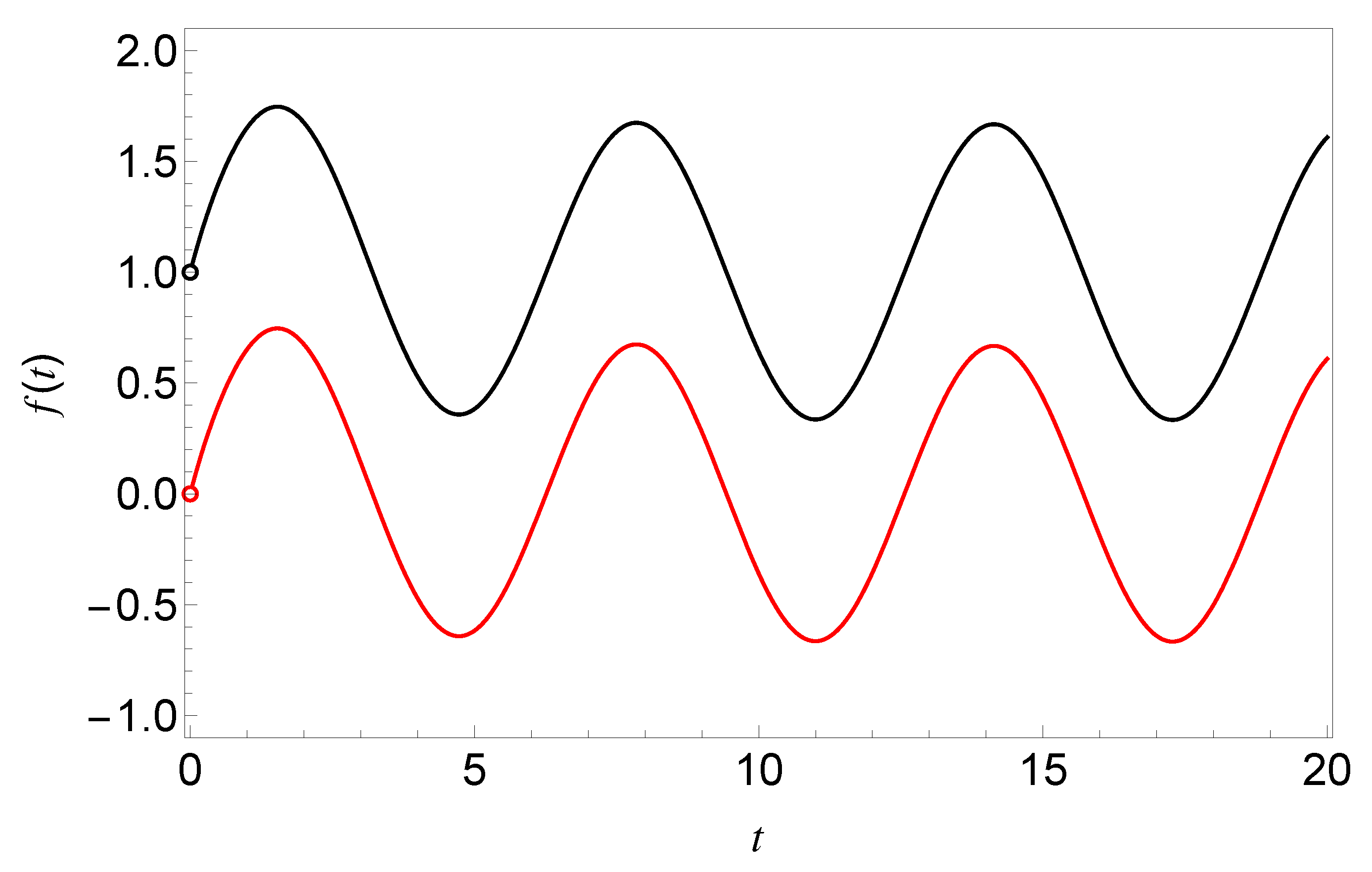
Corollary 2.

Suppose that; $K\left(t\right)$ and $G\left(t\right)$ are real-valued and bounded functions, continuous for $t\ge 0$ and differentiable for $t>0$; $K\left(0\right)\ne 0$; and $f\left(0\right)=f_0$. Then

$${}_0^{*}{\mathcal{D}}_{t}f\left(t\right)={\int }_0^{t}K(t-\tau )f^{\prime }\left(\tau \right)d\tau =G\left(t\right)-\frac{G\left(0\right)}{K\left(0\right)}K\left(t\right)$$

(33)

has a continuous and bounded solution for $t\ge 0$ given by

$$f\left(t\right)={\mathcal{L}}^{-1}\left[\frac{\widehat{G}\left(s\right)}{s\widehat{K}\left(s\right)}\right]\left(t\right)+f_0-\frac{G\left(0\right)}{K\left(0\right)}.$$

(34)

Examples of Caputo type IVPs and their solutions are given in Section 4. In general, we see that the non-singular kernel necessitates that the solution be discontinuous at $t=0$. This needs to be kept in mind for any application of these type of IVPs in modelling situations and otherwise.

3. Riemann–Liouville Type IVPs with Non-Singular Kernels

Next, we will consider the solutions to Riemann–Liouville type IVPs. We again begin with a definition.

Definition 2.

Suppose that; $K\left(t\right)$ and $G\left(t\right)$ are real-valued and bounded functions, continuous for $t\ge 0$ and differentiable for $t>0$; and $f\left(t\right)$ is a real-valued differentiable function, or generalized function that is differentiable in a distributional sense. Then a Riemann–Liouville type IVP of the first kind (RLI-IVP) is defined by the integro-differential equation

$${}_0{\mathcal{D}}_{t}f\left(t\right)=\frac{d}{dt}{\int }_0^{t}K(t-\tau )f\left(\tau \right)d\tau =G\left(t\right)$$

(35)

and the initial condition $f\left(0\right)=f_0$ with $f_0\in \mathbb{R}$.

It is helpful to first consider the special case where the IVP gives right-continuous solutions at the origin. Note that the condition here differs from the required condition on the right-hand side used in Lemma 1.

Lemma 2.

The solution of a RLI-IVP (Definition 2), with $K\left(0\right)\ne 0$ and $G\left(0\right)=K\left(0\right)f_0$, is given by

$$f\left(t\right)={\mathcal{L}}^{-1}\left[\frac{\widehat{G}\left(s\right)}{s\widehat{K}\left(s\right)}\right]\left(t\right)$$

(36)

and is right-continuous at $t=0$.

Proof. 

We first take the Laplace transform of Equation (35) to write

$$s\widehat{K}\left(s\right)\widehat{f}\left(s\right)=\widehat{G}\left(s\right).$$

(37)

Thus,

$$\widehat{f}\left(s\right)=\frac{\widehat{G}\left(s\right)}{s\widehat{K}\left(s\right)}$$

(38)

and

$$\begin{array}{cc}\hfill \underset{s\to \infty }{lim}s\widehat{f}\left(s\right)& =\underset{s\to \infty }{lim}\frac{s\widehat{G}\left(s\right)}{s\widehat{K}\left(s\right)}\hfill \end{array}$$

(39)

$$\begin{array}{cc}\hfill & =\underset{t\to 0}{lim}\frac{G\left(0\right)}{K\left(0\right)}\hfill \end{array}$$

(40)

$$\begin{array}{cc}\hfill & =\frac{K\left(0\right)f_0}{K\left(0\right)}\hfill \end{array}$$

(41)

$$\begin{array}{cc}\hfill & =f_0.\hfill \end{array}$$

(42)

It now also follows that

$$\underset{s\to \infty }{lim}\widehat{f}\left(s\right)=0.$$

(43)

The results in Equations (42) and (43) ensure that $f\left(t\right)={\mathcal{L}}^{-1}\left[\widehat{f}\left(s\right)\right]\left(t\right)$ exists and is right-continuous at $t=0$. □

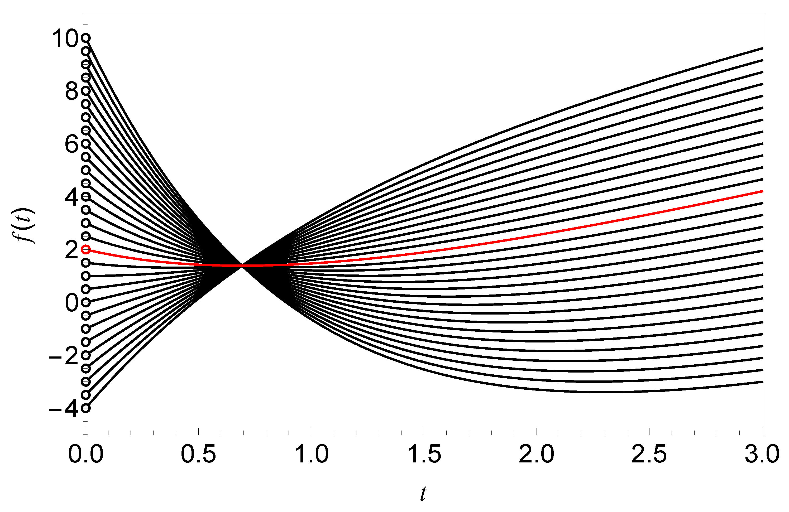
The general case again will display a discontinuity at the origin. It is interesting to note that as $f_0$ is varied the solution only shifts at $t=0$.

Theorem 2.

The solution of a RLI-IVP (Definition 2), with $K\left(0\right)\ne 0$, is given by

$$f\left(t\right)={\mathcal{L}}^{-1}\left[\frac{\widehat{G}\left(s\right)}{s\widehat{K}\left(s\right)}\right]\left(t\right)+\left(\frac{G\left(0\right)}{K\left(0\right)}-f_0\right)(H\left(t\right)-1),$$

(44)

where $H\left(t\right)$ is the Heaviside function defined in Equation (5).

Proof. 

The proof relies on establishing a relationship between Equations (13) and (35) and then utilizing Theorem 1. By interchanging the order of functions in the convolution and applying Leibniz rule for differentiation under the integral sign, we can write

$$\begin{array}{cc}\hfill \frac{d}{dt}{\int }_0^{t}K(t-\tau )f\left(\tau \right)d\tau & =\frac{d}{dt}{\int }_0^{t}K\left(\tau \right)f(t-\tau )d\tau \hfill \end{array}$$

(45)

$$\begin{array}{cc}\hfill & =K\left(t\right)f_0+{\int }_0^{t}K\left(\tau \right)f^{\prime }(t-\tau )d\tau \hfill \end{array}$$

(46)

$$\begin{array}{cc}\hfill & =K\left(t\right)f_0+{\int }_0^{t}K(t-\tau )f^{\prime }\left(\tau \right)d\tau .\hfill \end{array}$$

(47)

We now use the result of Equation (47) in Equation (35) and rearrange terms to re-write this as

$${\int }_0^{t}K(t-\tau )f^{\prime }\left(\tau \right)d\tau =M\left(t\right),$$

(48)

where $M\left(t\right)=G\left(t\right)-K\left(t\right)f_0$. It is noticed that this equation is of the same form as Equation (13) but with $G\left(t\right)$ replaced by $M\left(t\right)$. The final result, given by Equation (44), is then obtained by applying Theorem 1 to Equation (48). □

As an interesting exercise, an alternate proof of this theorem is given in Appendix A. The initial condition of the IVP only changes the solution at $t=0$. For $t>0$, with given functions K and G, the solutions are identical for all values of $f_0$. Similarly to the Caputo type case the special case where the kernel and right-hand side of the IVP are equal gives an interesting solution.

Corollary 3.

The solution of a RLI-IVP (Definition 2) for the special case in which $G\left(t\right)=K\left(t\right)$ is given by

$$f\left(t\right)=f_0+(1-f_0)H\left(t\right),$$

(49)

where $H\left(t\right)$ is the Heaviside function defined in Equation (5).

It is always possible to obtain continuous solutions to the IVP by the addition of a function on the right-hand side of the IVP that is equal to $f_{0}K\left(0\right)-G\left(0\right)$ when $t=0$. An example is given below.

Corollary 4.

Suppose that; $K\left(t\right)$ and $G\left(t\right)$ are real-valued and bounded functions, continuous at $t=0$ and differentiable for $t>0$; $K\left(0\right)\ne 0$; and $f\left(0\right)=f_0$. Then

$${}_0{\mathcal{D}}_{t}f\left(t\right)=\frac{d}{dt}{\int }_0^{t}K(t-\tau )f\left(\tau \right)d\tau =G\left(t\right)-\left(\frac{G\left(0\right)}{K\left(0\right)}-f_0\right)K\left(t\right)$$

(50)

has a continuous and bounded solution for $t\ge 0$ given by

$$f\left(t\right)={\mathcal{L}}^{-1}\left[\frac{\widehat{G}\left(s\right)}{s\widehat{K}\left(s\right)}\right]\left(t\right)+f_0-\frac{G\left(0\right)}{K\left(0\right)}.$$

(51)

In IVPs with continuous solutions, giving the initial condition as either $f\left(0\right)$ or ${lim}_{t\to 0}f\left(t\right)$ will be equivalent. This is not the case for either the Caputo or Riemann–Liouville type IVPs in general. Most interestingly, we find that the solution to Riemann–Liouville IVPs will propagate as a functional form of t. To find the solutions with this alternate form of initial condition, we will first define an alternate form to the IVP.

Definition 3.

Suppose that; $K\left(t\right)$ and $G\left(t\right)$ are real-valued and bounded functions, continuous for $t\ge 0$ and differentiable for $t>0$; and $f\left(t\right)$ is a real-valued differentiable function, or generalized function that is differentiable in a distributional sense. Then a Riemann–Liouville type IVP of the second kind (RLII-IVP) is defined by the integro-differential equation

$${}_0{\mathcal{D}}_{t}f\left(t\right)=\frac{d}{dt}{\int }_0^{t}K(t-\tau )f\left(\tau \right)d\tau =G\left(t\right)$$

(52)

and the limiting condition ${lim}_{t\to 0^{+}}f\left(t\right)=f_0$ with $f_0\in \mathbb{R}$.

Similar to the previous theorems, we see that the general case will display a discontinuity at the origin.

Theorem 3.

The solution of a RLII-IVP (Definition 3), with $K\left(0\right),K^{\prime }\left(0\right)\ne 0$, is given by

$$f\left(t\right)={\mathcal{L}}^{-1}\left[\frac{\widehat{G}\left(s\right)}{s\widehat{K}\left(s\right)}-\left(1-\frac{K\left(0\right)}{s\widehat{K}\left(s\right)}\right)\left(\frac{G\left(0\right)-f_{0}K\left(0\right)}{K^{\prime }\left(0\right)}\right)\right]\left(t\right)+\frac{G\left(0\right)-f_{0}K\left(0\right)}{K^{\prime }\left(0\right)}\delta \left(t\right),$$

(53)

where $\delta \left(t\right)$ is the Dirac delta generalized function.

Proof. 

The proof follows in a similar manner to that for Theorem 1. We begin by taking an ansatz solution of the form

$$f\left(t\right)=f_c\left(t\right)+b\delta \left(t\right),$$

(54)

where $f_c\left(t\right)$ is right-continuous at $t=0$ and differentiable for $t>0$ and b is a real-valued constant. We then note ${lim}_{t\to 0^{+}}f\left(t\right)=f_c\left(0\right)$, or equivalently, $f_c\left(0\right)=f_0$. Substitution of the ansatz solution into Equation (52) gives

$$\frac{d}{dt}{\int }_0^{t}K(t-\tau )f_c\left(\tau \right)d\tau =G\left(t\right)-b{K}^{\prime }\left(t\right).$$

(55)

To find an explicit expression for the constant b we consider the limit $t\to 0$ and employ the initial value theorem to find that the integral over classical functions gives

$$\underset{t\to 0}{lim}\frac{d}{dt}{\int }_0^{t}K(t-\tau )f_c\left(\tau \right)d\tau =\underset{s\to \infty }{lim}\left(s\widehat{K}\left(s\right)·s\widehat{f_c}\left(s\right)\right)=K\left(0\right)f_0.$$

(56)

Thus, we require

$$b=\frac{G\left(0\right)-f_{0}K\left(0\right)}{K^{\prime }\left(0\right)}.$$

(57)

Substituting this expression for b into Equation (55) yields

$$\frac{d}{dt}{\int }_0^{t}K(t-\tau )f_c\left(\tau \right)d\tau =N\left(t\right),$$

(58)

where

$$N\left(t\right)=G\left(t\right)-\left(\frac{G\left(0\right)-f_{0}K\left(0\right)}{K^{\prime }\left(0\right)}\right)K^{\prime }\left(t\right).$$

(59)

It is noticed that Equation (58) is of the same form as Equation (35) with $G\left(t\right)$ replaced by $N\left(t\right)$ and $N\left(0\right)=f_{0}K\left(0\right)$. Since $f_c\left(t\right)$ is is right-continuous at $t=0$, we know that the initial and limiting condition are equal. Hence, we can utilize Lemma 2 to find

$$f_c\left(t\right)={\mathcal{L}}^{-1}\left[\frac{\widehat{G}\left(s\right)}{s\widehat{K}\left(s\right)}-\left(1-\frac{K\left(0\right)}{s\widehat{K}\left(s\right)}\right)\left(\frac{G\left(0\right)-f_{0}K\left(0\right)}{K^{\prime }\left(0\right)}\right)\right]\left(t\right).$$

(60)

Thus, the final result, given by Equation (53), is then obtained by substituting Equations (57) and (60) into Equation (54). □

As an interesting exercise, an alternate proof of this theorem is given in Appendix A. Again we can modify the IVP to ensure that solutions are continuous by the addition of a function on the right-hand side that is equal to $f_{0}K\left(0\right)-G\left(0\right)$ when $t=0$. An example of this is given below.

Corollary 5.

Suppose that; $K\left(t\right)$ and $G\left(t\right)$ are real-valued and bounded functions, continuous for $t\ge 0$ and differentiable for $t>0$; $K\left(0\right),K^{\prime }\left(0\right)\ne 0$; and ${lim}_{t\to 0^{+}}f\left(t\right)=f_0$. Then

$${}_0{\mathcal{D}}_{t}f\left(t\right)=\frac{d}{dt}{\int }_0^{t}K(t-\tau )f\left(\tau \right)d\tau =G\left(t\right)-\left(\frac{G\left(0\right)-f_{0}K\left(0\right)}{K^{\prime }\left(0\right)}\right)K^{\prime }\left(t\right).$$

(61)

has a continuous and bounded solution for $t\ge 0$ given by

$$f\left(t\right)={\mathcal{L}}^{-1}\left[\frac{\widehat{G}\left(s\right)}{s\widehat{K}\left(s\right)}-\left(1-\frac{K\left(0\right)}{s\widehat{K}\left(s\right)}\right)\left(\frac{G\left(0\right)-f_{0}K\left(0\right)}{K^{\prime }\left(0\right)}\right)\right]\left(t\right).$$

(62)

4. Examples

In this section we present some examples of solutions to generalized Caputo and Riemann–Liouville type IVPs with non-singular kernels. In general, the solutions to RLI-IVPs and RLII-IVPs are equivalent for the special case in which the solution is right-continuous at $t=0$. This can be seen from the initial condition, since ${lim}_{t\to 0^{+}}f\left(t\right)=f\left(0\right)$ by the right-continuity of f. The solution to each example can be easily verified via direct substitution into the respective IVP.

4.1. C-IVP with $K\left(t\right)=1-t^2$

Consider the C-IVP with

$${\int }_0^t\left(1-{(t-\tau )}^2\right)f^{\prime }\left(\tau \right)d\tau =cos\left(t\right)exp(-t)\mathrm{and}f\left(0\right)=f_0$$

(63)

with $f_0\in \mathbb{R}$. The solution of this IVP is given by

$$f\left(t\right)=f_0-1+\frac{1}{2}\left(cosh\left(\sqrt{2}t\right)+exp\left(t\right)\left(cos\left(t\right)+sin\left(t\right)\right)\right)+H\left(t\right).$$

(64)

Notice that the solution has a discontinuity at $t=0$.

4.2. C-IVP with $K\left(t\right)=1+texp(-t)$

Consider the C-IVP

$${\int }_0^t\left(1+(t-\tau )exp(\tau -t)\right)f^{\prime }\left(\tau \right)d\tau =sin\left(t\right)\mathrm{and}f\left(0\right)=f_0,$$

(65)

with $f_0\in \mathbb{R}$. The solution of this IVP is given by

$$f\left(t\right)=f_0+\frac{2}{3}sin\left(t\right)+\frac{2\sqrt{5}}{15}exp\left(\frac{-3t}{2}\right)sinh\left(\frac{\sqrt{5}t}{2}\right).$$

(66)

This solution is continuous for all $t\in \mathbb{R}$, which is expected as $G\left(t\right)=sin\left(t\right)$ vanishes at $t=0$.

4.3. RLI-IVP with $K\left(t\right)=cos\left(t\right)+sin\left(t\right)$

Consider the RLI-IVP with

$$\frac{d}{dt}{\int }_0^t\left(cos(t-\tau )+sin(t-\tau )\right)f\left(\tau \right)d\tau =g\mathrm{and}f\left(0\right)=f_0$$

(67)

with $g,f_0\in \mathbb{R}$. The solution of this IVP is given by

$$f\left(t\right)=f_0+\left(t-2+2exp(-t)\right)g+(g-f_0)H\left(t\right).$$

(68)

Notice that the solution has a discontinuity at $t=0$ unless $g=f_0$.

4.4. RLI-IVP with $K\left(t\right)=1+texp(-t)$

Consider the RLI-IVP with

$$\frac{d}{dt}{\int }_0^t\left(1+(t-\tau )exp(\tau -t)\right)f\left(\tau \right)d\tau =sin\left(t\right)\mathrm{and}f\left(0\right)=f_0$$

(69)

with $f_0\in \mathbb{R}$. The solution of this IVP is given by

$$f\left(t\right)=f_0+\frac{2}{3}sin\left(t\right)+\frac{2\sqrt{5}}{15}exp\left(\frac{-3t}{2}\right)sinh\left(\frac{\sqrt{5}t}{2}\right)-f_{0}H\left(t\right).$$

(70)

This solution has a discontinuity at $t=0$ unless $f_0=0$. When $t>0$, we see that Equation (70) is independent of the initial value $f_0$ and the difference between Equations (66) and (70) is equal to the precise value of $f_0$. This is illustrated in Figure 1, where there is a vertical shift of $f_0=1$ for the curve representing Equation (66) from the curve representing Equation (70). For the special case in which $f_0=0$, then Equation (66) is equivalent to Equation (70). This is true in general, where Equation (23) is equivalent to Equation (44) when $f_0=0$.

4.5. RLII-IVP with $K\left(t\right)=exp\left(\frac{\beta }{\beta -1}t\right)$

Consider the RLII-IVP

$$\frac{d}{dt}{\int }_0^{t}exp\left(\frac{\beta }{\beta -1}(t-\tau )\right)f\left(\tau \right)d\tau =g\mathrm{and}\underset{t\to 0^{+}}{lim}f\left(t\right)=f_0$$

(71)

with $g,f_0\in \mathbb{R}$ and $\beta >1$. The solution of this IVP is given by

$$f\left(t\right)=f_0-\frac{\beta gt}{\beta -1}+\frac{(g-f_0)(\beta -1)}{\beta }\delta \left(t\right).$$

(72)

Notice that we have ${lim}_{t\to 0^{+}}f\left(t\right)=f_0$ but due to the Dirac delta $f\left(0\right)\ne f_0$ unless $f_0=g$.

4.6. RLII-IVP with $K\left(t\right)=cos\left(t\right)+sin\left(t\right)$

Consider the RLII-IVP with

$$\frac{d}{dt}{\int }_0^t\left(cos(t-\tau )+sin(t-\tau )\right)f\left(\tau \right)d\tau =g\mathrm{and}\underset{t\to 0^{+}}{lim}f\left(t\right)=f_0$$

(73)

with $g,f_0\in \mathbb{R}$. The solution of this IVP is given by

$$f\left(t\right)=gt+\left(2exp(-t)-1\right)f_0+(g-f_0)\delta \left(t\right).$$

(74)

In contrast to Equation (68), we see that Equation (74) is dependent on the initial value $f_0$. Consequently, varying $f_0$ will affect the form of Equation (74). This is illustrated in Figure 2, where the curves representing Equation (74) vary according to the specific value of $f_0$ and the curve representing Equation (68) remains unchanged. For the special case in which $g=f_0$, Equation (68) is equivalent to Equation (74).

5. Summary and Discussion

Here we have considered IVPs for integro-differential equations of the form ${\mathcal{D}}_{t}f\left(t\right)=G\left(t\right)$ where the operator ${\mathcal{D}}_t$ is either similar to the Riemann–Liouville derivative, or similar to the Caputo derivative, but with the singular kernel in those operators replaced by a non-singular kernel $K\left(t\right)$, and $K\left(0\right)\ne 0$. We have not attempted to motivate this replacement by modelling considerations; rather, we have sought to understand what the implications of such replacements would be in modelling applications. Our motivation in this pursuit has been guided by the plethora of integro-differential operators that have been introduced in recent years. In modelling applications, it would be expected that $G\left(t\right)$ and $K\left(t\right)$ are prescribed functions, and $f\left(t\right)$ is unknown except at the origin. We find that the IVPs for these integro-differential equations with non-singular kernels, in general, have solutions that have intrinsic discontinuities at the origin. We also show that it is possible to re-formulate these IVPs so that solutions are guaranteed to be continuous at the origin but this comes at the cost of effectively constraining the right-hand side of the equations so that they are no longer just dependent on the prescribed function $G\left(t\right)$. These results are problematic for modelling applications which would seek to employ Riemann–Liouville type, or Caputo type, differential operators but with the singular kernel replaced by a non-singular kernel.

References

1. De Oliveira, E.C.; Tenreiro Machado, J.A. A Review of Definitions for Fractional Derivatives and Integral. Math. Probl. Eng. 2014, 2014, 238459. [Google Scholar] [CrossRef] [Green Version]
2. Li, C.; Qian, D.; Chen, Y. On Riemann-Liouville and Caputo Derivatives. Discret. Dyn. Nat. Soc. 2011, 2011, 562494. [Google Scholar] [CrossRef] [Green Version]
3. Ortigueira, M.D. A new look at the initial condition problem. Mathematics 2022, 10, 1771. [Google Scholar] [CrossRef]
4. Caputo, M.; Fabrizio, M. A new definition of fractional derivative without singular kernel. Prog. Fract. Differ. Appl. 2015, 1, 73–85. [Google Scholar]
5. Losada, J.; Nieto, J.J. Properties of a new fractional derivative without singular kernel. Prog. Fract. Differ. Appl. 2015, 1, 87–92. [Google Scholar]
6. Atangana, A.; Baleanu, D. New fractional derivatives with non-local and non-singular kernel. Themal Sci. 2016, 20, 763–769. [Google Scholar] [CrossRef] [Green Version]
7. Ortigueira, M.D.; Tenreiro Machado, J. A critical analysis of the Caputo-Fabrizio operator. Commun. Nonlinear Sci. Numer. Simul. 2018, 59, 608–611. [Google Scholar] [CrossRef]
8. Tarasov, V.E. Caputo–Fabrizio operator in terms of integer derivatives: Memory or distributed lag? Comput. Appl. Math. 2019, 38, 113. [Google Scholar] [CrossRef]
9. Hanyga, A. A comment on a controversial issue: A generalized fractional derivative cannot have a regular kernel. Fract. Calc. Appl. Anal. 2020, 23, 211–223. [Google Scholar] [CrossRef] [Green Version]
10. Angstmann, C.N.; Jacobs, B.A.; Henry, B.I.; Xu, Z. Intrinsic discontinuities in solutions of evolution equations involving fractional Caputo–Fabrizio and Atangana–Baleanu operators. Mathematics 2020, 8, 2023. [Google Scholar] [CrossRef]
11. Faleleev, M.V.; Sidorov, N.A.; Sidorov, D.N. Generalized solutions of Volterra integral equations of the first kind. Lobachevskii J. Math. 2005, 20, 47–57. [Google Scholar]
12. Sidorov, N.A.; Sidorov, D.N. Existence and construction of generalized solutions of nonlinear Volterra integral equations of the first kind. Differ. Equ. 2006, 42, 1312–1316. [Google Scholar] [CrossRef]
13. Ziemanian, A.H. An introduction to generalized functions and the generalized Laplace and Legendre transformations. SIAM Rev. 1968, 10, 1–24. [Google Scholar] [CrossRef]
Figure 1. The black and red curves represent the IVP solutions given by Equations (66) and (70) respectively with f 0 = 1 . The open circle on each curve indicates that both solutions are valid for t > 0 .
Fractalfract 06 00436 g001
Figure 2. The black and red curves represent the IVP solutions given by Equations (68) and (74) respectively for varying values of f 0 with g = 2 . The open circle on each curve indicates that both solutions are valid for t > 0 .
Fractalfract 06 00436 g002
Publisher’s Note: MDPI stays neutral with regard to jurisdictional claims in published maps and institutional affiliations.