A Bi-Geometric Fractional Model for the Treatment of Cancer Using Radiotherapy

Abstract

Our study is based on the modification of a well-known predator-prey equation, or the Lotka–Volterra competition model. That is, a system of differential equations was established for the population of healthy and cancerous cells within the tumor tissue of a patient struggling with cancer. Besides, fractional differentiation remedies the situation by obtaining a meticulous model with more flexible parameters. Furthermore, a specific type of non-Newtonian calculus, bi-geometric calculus, can describe the model in terms of proportions and implies the alternative aspect of a dynamic system. Moreover, fractional operators in bi-geometric calculus are formulated in terms of Hadamard fractional operators. In this article, the development of fractional operators in non-Newtonian calculus was investigated. The model was extended in these criteria, and the existence and uniqueness of the model were considered and guaranteed in the first step by applying the Arzelà–Ascoli. The bi-geometric analogue of the numerical method provided a suitable tool to solve the model approximately. In the end, the visual graphs were obtained by using the MATLAB program.

1. Introduction

Cancer is a fatal disease: the last updates of cancer incidence and mortality showed that an estimated 19.3 million new cancer cases and almost 10 million cancer deaths occurred in 2020 [1]. Broadly speaking, there are many areas where theory has contributed the most to cancer research and these areas were classified into three major parts [2]. One of the oldest and best developed topics in biomathematics is the mathematical modeling of growth with consideration of differentiation, and mutations of cells in tumors. The dynamic system that contains the population of healthy and cancerous cells can be interpreted as an ecological system [3,4,5]. This correspondence implies the usage of Lotka–Volterra equations to describe the competition between healthy and cancerous cells in the struggling tissue [6,7]. Roughly speaking, the treatment methods for cancer can be categorized into four different methods, namely, surgery, chemotherapy, radiotherapy, and immunotherapy. These treatment methods can be considered as some factors in the system of equations. Furthermore, fractional derivative can be seen as an alternative to ordinary derivative and ODE (ordinary differential equation) can be replaced by FDE (fractional differential equation) to obtain a better fitting function with non-local properties [8,9,10,11]. There are different types of fractional operators and each comes from a different origin with some interesting properties but mainly the Reimann–Liouville type is used to model most of the real phenomena due to the compatible attitude of this operator with Newtonian calculus. Newtonian calculus refers to the formulation of arithmetic operators on this field and the alternative ways determine non-Newtonian calculi. One of the most famous non-Newtonian calculi is called bi-geometric calculus and it is equipped with the Hadamard fractional operator [12,13]. There are some attempts to model cancer treatments by using the Hadamard fractional operators, but the reliable method needs profound investigation into the nature of the calculus that is used [14].

The outline of this paper is as follows: The first section involves the development of concepts in non-Newtonian calculi, and through this debate, the special case, bi-geometric calculus, is more emphasized. Generally, we stress historical origin when it is helpful. The second section contains a glimpse of biological contents that lead to stating a dynamic system of healthy and cancerous cell populations in terms of bi-geometric calculus. Therefore, the fractional bi-geometric model and its uniqueness and existence are considered in this chapter. In the last chapter the numerical solution is introduced. Indeed, the bi-geometric analogue of numerical methods for Reimann–Liouville operators extends the methods for Hadamard operators with the logarithmic-weighted integral.

2. Non-Newtonian Calculi and Fractional Operators

The real numbers can be assumed as a complete set with two binary operators and the order on the set. Most mathematical systems are sets with some binary operations, some relations, or distinguished subsets. In this analogy, without any sort of tacit, we can demonstrate the real set as a quadruple $(R,+,-,<)$. Here, the real system with these binary operators and inequality satisfies the axioms of a complete Archimedean ordered field. The main idea of non-Newtonian calculi can be summarized by modifying the arithmetic operators. For instance, replacing addition with multiplication and subtraction with division can result in a new calculus which is called the multiplicative calculus or geometric calculus. Here, many things are changed, such as arithmetic means to geometric means and etc. Generally, if we denote the arithmetic operators $\left(+,-,\times , /\right)$ by ⋆ then corresponding operators on non-Newtonian calculi can be rewritten as

$$a{⊛}_{\alpha }b=\alpha \left({\alpha }^{-1}\left(a\right)\star {\alpha }^{-1}\left(b\right)\right)$$

As far as we know, the original idea belongs to Michael Grossman and Robert Katz, who introduced the non-Newtonian calculus in 1972 in a book titled non-Newtonian calculi [15]. Almost simultaneously, E. Pop was inspired by t-conorm decomposable measures and defined g-calculus by putting $g^{-1}\left(x\right)$ instead of $\alpha \left(x\right)$ and these binary operators were named Pseudo-operators [16,17]. These two different analogies of the same concept were developed quite separately in different aspects. It is a safe bet that researchers in these two branches have not found out the similarity of the concept, and the consequence is that many articles with the same purpose have been published with different notations [18,19]. Besides, there is no consensus about the conditions generally in both approaches. Indeed, the function $\alpha \left(x\right)$ plays the role of converting between different calculi and maintaining the algebraic structure of real numbers, which is overly related to the properties of an invertible function. Here, if we want to emphasize on preserving topological properties, we should consider $\alpha \left(x\right)$ as a bijection. Furthermore, being differentiable is necessary to meet the need for defining the derivative in non-Newtonian calculus. Fortunately, the exponential function satisfies all these conditions and is even analytic for complex values. With these criteria, the general derivative and integral can be rewritten as [12]

$${}_{}{}^{\alpha \left(x\right)}D\left(f\right)\left(x\right)=f^{\widehat{\alpha }}\left(x\right)=\underset{y\to x}{\lim }\left(\left(f\left(y\right){⊝}_{\alpha }f\left(x\right)\right){\oslash }_{\alpha }\left(y{⊝}_{\alpha }x\right)\right)=\alpha \left(\frac{{\alpha }^{-1}{\left(f\left(x\right)\right)}^{\prime }}{{\alpha }^{-1}{\left(x\right)}^{\prime }}\right),$$

$$\begin{array}{c}{}_{}{}^{\alpha \left(x\right)}I\left(f\right)\left(x\right)={\int }_a^{x}f\left(t\right)d^{\widehat{\alpha }}t=\underset{n\to \infty }{\lim }{}_n{}^{i=1}⨁_{\alpha }\left(\left(f\left(c_i\right){⨂}_{\alpha }\left(x_{i+1}{⊝}_{\alpha }{x}_i\right)\right)\right)\\ =\alpha \left({\int }_a^x{\alpha }^{-1}\left(f\left(t\right)\right){\alpha }^{-1}{\left(t\right)}^{\prime }dt\right).\end{array}$$

Using h-derivative or applying the formula as we mentioned above, we can obtain a derivative formula from two different limits. In particular, if we consider the exponential function, then two different formulas will come out as

$${}_{}{}^{\exp }D\left(f\right)\left(x\right)=f^{*}\left(x\right)=\underset{y\to x}{\lim }\sqrt[ln\left(\frac{y}{x}\right)]{\frac{f\left(y\right)}{f\left(x\right)}}=\exp \left(\frac{x{\left(f\left(x\right)\right)}^{\prime }}{f\left(x\right)}\right)$$

$${}_{}{}^{\exp }D{}^o\left(f\right)\left(x\right)=f^o\left(x\right)=\underset{h\to 0}{\lim }\sqrt[lnh]{\frac{f\left(x+h\right)}{f\left(x\right)}}=\exp \left(\frac{{\left(f\left(x\right)\right)}^{\prime }}{f\left(x\right)}\right)$$

Due to the usage of pairs of distinct values in the forms of $f\left(x\right)$ and $f\left(y\right)$, to compute the derivative in the first formula, $f^{*}\left(x\right)$ is called the bi-geometric derivative, and the derived formula from h-derivative, $f^o\left(x\right)$, is called the geometric derivative or multiplicative derivative [20]. In fact, the multiplicative derivative, $f^o\left(x\right)$, has its own interpretation as a positive number, which represents how many times $f\left(x\right)$ increases at the moment x or the growth factor at the moment x [21]. This interpretation helps us understand the attitude of the function and leads to some applications in actuarial science, economics, biology, demography, etc. For instance, in a specific part of our model, logistic growth is used, which can be considered generally as

$${}_{}{}^{\exp }D{}^o\left(N\right)\left(t\right)=\exp \left(\frac{\beta }{a}\left(1-{\left(\frac{N}{K}\right)}^a\right)\right),N\left(t=0\right)=N_o>0$$

Here, $\beta$ denotes the proliferation factor, and $K>0$ represents the carrying capacity of the population, and in the case of catching the value, the multiplicative derivative equals to one that interprets the only single increase in the population function. Almost the entire exponential growth of small tumors and growth saturation can be predicted by the logistic growth law when $a=1$. Furthermore, $a \to 0^{+}$ obtains the Gompertzian growth law, which is considered in terms of multiplicative calculus in [21]. Besides, this method of demonstration does not reformulate the old version of the population’s model. Indeed, because of the nature of exponential functions, negative values in the interval $\left[0, 1\right]$ are shrunk, and the allocated calculus only deals with positive values. Moreover, it is essential, or rather obligatory, to express the model in non-dimensional terms, and writing the function in terms of proportions prepares the non-dimensional terms. This has several advantages. For example, the units used in the analysis are then unimportant, and the adjectives “small” and “large” have a definite relative meaning. It also always reduces the number of relevant parameters to dimensionless groupings that determine the dynamics.

Fractional Operators on Non-Newtonian Calculus

The primary goal of fractional calculus is to define the derivative of the function in any order, preferably the complex number. This idea could be traced back to letters that were written between L’Hopital and Leibniz in 1695 and assumed as the birth day of fractional calculus. In 1823, N. H. Abel was studying the tautochrone problem of mechanics, the problem of which, in the absence of friction, is reduced to that of solving the equation as [22]

$${\int }_0^y{\left(y-z\right)}^{-\frac{1}{2}}u\left(z\right)dz=\sqrt{2g}t\left(y\right),y\in \left[0,H\right]$$

where $u\left(z\right)=\sqrt{1+{\varphi }^2{\left(z\right)}^{\prime }}$ and $x=\varphi \left(y\right)$ is an increasing function, under constant downward acceleration of $g$, a particle must be constrained to fall, in order that its falling time equals a prescribed function $t\left(\overline{y}\right)$ of the initial height $\overline{y}$. Indeed, he treated a more general equation by replacing ${\left(y-z\right)}^{-\frac{1}{2}}$ with ${\left(y-z\right)}^{\mu -1}$ (for $0<\mu <1$). In fact, this equation was one of the first integral equations ever treated, and in honor of V. Volterra, the more general type is called the singular Volterra equation of the first kind. This integral equation has a kernel with a singularity of the type ${\left(y-z\right)}^{\mu -1}$. In 1892, Hadamard published a series of articles and investigated the singularity of the integral equation. In the third part of these publications, Hadamard investigated the relation between the coefficients of a series with a unit radius of convergent and treated the Reimann operator by using logarithmic functions as a kernel of the Volterra integral [23]. The Reimann and Hadamard fractional integrals are known as follows:

$${}_a{}^{}I{}_x^{\mu }\left(f\right)\left(x\right)=\frac{1}{\mathsf{\Gamma }\left(\mu \right)}{\int }_a^x{\left(x-s\right)}^{\mu -1}f\left(s\right)ds$$

$${}_a{}^{H}J{}_x^{\mu }\left(f\right)\left(x\right)=\frac{1}{\mathsf{\Gamma }\left(\mu \right)}{\int }_a^x{\left(ln\left(\frac{x}{s}\right)\right)}^{\mu -1}f\left(s\right)\frac{ds}{s}$$

The idea of the fractional integral in terms of any arbitrary function was well developed in the remarkable works of Osler, which led to the $\mathrm{\Psi }$-fractional differential operators [24]. The key point of Osler’s discussion was applying the general Leibniz formula to derive the fractional derivative of a composite function. The general Leibniz formula and product rule of non-Newtonian calculus can be written respectively as follows

$$D_{g\left(z\right)}{}^n\left(u\left(x\right)·v\left(x\right)\right)={\displaystyle \sum _{k=0}^n}\left(\begin{array}{c}n\\ k\end{array}\right)D_{g\left(z\right)}{}^k\left(u\left(x\right)\right)D_{g\left(z\right)}{}^{n-k}\left(v\left(x\right)\right)=$$

$${\displaystyle \sum _{k=0}^n}\left(\begin{array}{c}n\\ k\end{array}\right){\left(\frac{1}{g{\left(x\right)}^{\prime }}\frac{d}{dx}\right)}^k\left(u\left(x\right)\right){\left(\frac{1}{g{\left(x\right)}^{\prime }}\frac{d}{dx}\right)}^{n-k}\left(v\left(x\right)\right),$$

$$\begin{array}{c}{{}_{}{}^{\alpha \left(x\right)}D}^n\left(u\left(x\right){\otimes }_{\alpha }v\left(x\right)\right)=\alpha \left({\left(\frac{1}{{\alpha }^{-1}{\left(x\right)}^{\prime }}\frac{d}{dx}\right)}^n\left({\alpha }^{-1}ou\left(x\right)·{\alpha }^{-1}ov\left(x\right)\right)\right)\\ ={}_{k=0}{}^n\oplus _{\alpha \left(x\right)}\left(\alpha \left(\frac{n!}{k!\left(n-k\right)!}\right){\otimes }_{\alpha }{D}^k\left(u\left(x\right)\right){\otimes }_{\alpha }{D}^{n-k}\left(v\left(x\right)\right)\right)\\ =\alpha \left({\displaystyle \sum _{k=0}^n}\left(\begin{array}{c}n\\ k\end{array}\right){\left(\frac{1}{{\alpha }^{-1}{\left(x\right)}^{\prime }}\frac{d}{dx}\right)}^k\left({\alpha }^{-1}ou\left(x\right)\right){\left(\frac{1}{{\alpha }^{-1}{\left(x\right)}^{\prime }}\frac{d}{dx}\right)}^{n-k}\left({\alpha }^{-1}ov\left(x\right)\right)\right).\end{array}$$

There are different approaches to fractional operators. One may use the Cauchy iterated integrals to define the fractional order of integration, or one may follow Osler’s method to define the fractional derivative. For instance, katugambola applied the polynomials in the chains of iterated integrals to make the general forms of fractional integral operators. Similarly, we can make the fractional operators for non-Newtonian calculi, and the results can be seen as

$${\displaystyle \underset{a}{\overset{x}{\int }}}{d}^{\widehat{\alpha }}{t}_1{\displaystyle \underset{a}{\overset{t_1}{\int }}}{d}^{\widehat{\alpha }}{t}_2\dots {\displaystyle \underset{a}{\overset{t_{n-1}}{\int }}}f\left(t_n\right)d^{\widehat{\alpha }}{t}_n=\alpha \left(\frac{1}{\left(n-1\right)!}{\displaystyle \underset{a}{\overset{x}{{\displaystyle \int }}}}{\left({\alpha }^{-1}\left(x\right)-{\alpha }^{-1}\left(s\right)\right)}^{n-1}{\alpha }^{-1}\left(f\left(s\right)\right){\alpha }^{-1}{\left(s\right)}^{\prime }ds\right)$$

The resulting operators have a close resemblance to fractional operators with respect to any functions. However, fractional operators on non-Newtonian calculi are the natural extension of these operators in the corresponding calculi. Moreover, there are two different types of fractional derivatives that can be considered as a result of the different orders of action of the derivative and integral. The Reimann fractional derivative is the analytic continuum of order, and the fractional integral is first applied to the function, and then the natural order derivative will be taken. Thus, this fractional derivative can be considered as a natural extension of the fundamental theorem of calculus. On the other hand, the Caputo fractional derivative results from applying the natural order derivative first, and then the fractional integral. Due to the uniqueness of the inverse analytic continuum operator in their order, the Caputo derivative does not have the same properties as inverse operators. However, the initial values in FDE that use the Caputo derivative are more convenient to describe the real phenomena. In the following

Table 1. Comparison of differentiation operators in different Calculi.

Type of Calculus	Derivative (μ = 1)	Integral (μ = −1)
Newtonian	$f^{\prime }\left(x\right)$	${}_a{}^{}I{}_x\left(f\right)\left(x\right)={{\displaystyle \int }}_a^{x}f\left(s\right)ds$
Bi-Geometric	$f^{*}\left(x\right)=\exp \left(\frac{x\left(f\left(x\right)\right){}^{\prime }}{f\left(x\right)}\right)$	${}_a{}^{\mathrm{e}\mathrm{x}\mathrm{p}\left(x\right)}I{}_x\left(f\right)\left(x\right)=\exp \left({{\displaystyle \int }}_a^{x}ln\left(f\left(s\right)\right)\frac{ds}{s}\right)$
$t^p$-calculus	$f^{\left(p\right)}\left(x\right)=\frac{{\left(f\left(x\right)\right)}^q{\left(f\left(x\right){}^{\prime }\right)}^p}{x^q}, \frac{1}{p}+\frac{1}{q}=1$	${}_a{}^{x^p}I{}_x\left(f\right)\left(x\right)={\left(\frac{1}{p}{{\displaystyle \int }}_a^x{f}^{\frac{1}{p}}\left(s\right)s^{\frac{1}{q}}ds\right)}^p$
Bi-Positive Calculus	$f^{\left(\mathcal{l}\right)}\left(x\right)=ln\left(f{\left(x\right)}^{\prime }\right)+f\left(x\right)-x$	${}_a{}^{ln\left(x\right)}I{}_x\left(f\right)\left(x\right)=ln\left({{\displaystyle \int }}_a^x\mathrm{e}\mathrm{x}\mathrm{p}\left(sf\left(s\right)\right)ds\right)$
$\alpha$-Calculus	${}_{}{}^{\alpha \left(x\right)}D\left(f\right)\left(x\right)=\alpha \left(\frac{{\alpha }^{-1}\left(f\left(x\right)\right){}^{\prime }}{{\alpha }^{-1}\left(x\right){}^{\prime }}\right)$	${}_a{}^{\alpha \left(x\right)}I{}_x\left(f\right)\left(x\right)=\alpha \left({{\displaystyle \int }}_a^x{\alpha }^{-1}\left(f\left(s\right)\right){\alpha }^{-1}\left(s\right){}^{\prime }ds\right)$
Type of Calculus	Fractional Integral (μ)
Newtonian	${}_a{}^{}I{}_x^{\mu }\left(f\right)\left(x\right)=\frac{1}{\Gamma \left(\mu \right)}{\int }_a^x{\left(x-s\right)}^{\mu -1}f\left(s\right)ds$
Bi-Geometric	${}_a{}^{\mathrm{e}\mathrm{x}\mathrm{p}}I{}_x^{\mu }\left(f\right)\left(x\right)=\mathrm{e}\mathrm{x}\mathrm{p}\left(\frac{1}{\Gamma \left(\mu \right)}{\int }_a^x{\left(ln\left(\frac{x}{s}\right)\right)}^{\mu -1}ln\left(f\left(s\right)\right)\frac{ds}{s}\right)$
$t^p$-calculus	${}_a{}^{x^p}I{}_x^{\mu }\left(f\right)\left(x\right)={\left(\frac{1}{p\Gamma \left(\mu \right)}{{\displaystyle \int }}_a^x{\left(x^{\frac{1}{p}}-s^{\frac{1}{p}}\right)}^{\mu -1}{f}^{\frac{1}{p}}\left(s\right)s^{\frac{1}{q}}ds\right)}^p$
Bi-Positive Calculus	${}_a{}^{ln}I{}_x^{\mu }\left(f\right)\left(x\right)=ln\left(\frac{1}{\Gamma \left(\mu \right)}{{\displaystyle \int }}_a^x{\left(e^x-e^s\right)}^{\mu -1}\mathrm{e}\mathrm{x}\mathrm{p}\left(f\left(s\right)+s\right)ds\right)$
$\alpha$-Calculus	${}_a{}^{}I{}_x^{\mu }\left(f\right)\left(x\right)=\alpha \left(\frac{1}{\Gamma \left(\mu \right)}{{\displaystyle \int }}_a^x{\left({\alpha }^{-1}\left(x\right)-{\alpha }^{-1}\left(s\right)\right)}^{\mu -1}{\alpha }^{-1}\left(f\left(s\right)\right){\alpha }^{-1}\left(s\right)\right)$
Type of Calculus	Caputo Fractional Derivative (−μ)
Newtonian	${}_a{}^{C}D{}_x^{\mu }\left(f\right)\left(x\right)=\frac{1}{\Gamma \left(n-\mu \right)}{{\displaystyle \int }}_a^x{\left(x-s\right)}^{n-\mu -1}{f}^{\left(n\right)}\left(s\right)ds$
Bi-Geometric	${}_a{}^{\mathrm{e}\mathrm{x}\mathrm{p}}D{}_x^{\mu }\left(f\right)\left(x\right)=\mathrm{e}\mathrm{x}\mathrm{p}\left(\frac{1}{\Gamma \left(n-\mu \right)}{{\displaystyle \int }}_a^x{\left(ln\left(\frac{x}{s}\right)\right)}^{n-\mu -1}{\left(s\frac{d}{ds}\right)}^{n}ln\left(f\left(s\right)\right)\frac{ds}{s}\right)$
$t^p$-calculus	${}_a{}^{x^p}D{}_x^{\mu }\left(f\right)\left(x\right)={\left(\frac{1}{\Gamma \left(n-\mu \right)}{{\displaystyle \int }}_a^x{\left(x^{\frac{1}{p}}-s^{\frac{1}{p}}\right)}^{n-\mu -1}{\left(\frac{1}{p}{s}^{\frac{1}{q}}\frac{d}{ds}\right)}^n{f}^{\frac{1}{p}}\left(s\right)s^{\frac{1}{q}}ds\right)}^p$
Bi-Positive Calculus	${}_a{}^{ln}D{}_x^{\mu }\left(f\right)\left(x\right)=ln\left(\frac{1}{\Gamma \left(n-\mu \right)}{{\displaystyle \int }}_a^x{\left(e^x-e^s\right)}^{n-\mu -1}{\left(e^s\frac{d}{ds}\right)}^n\mathrm{e}\mathrm{x}\mathrm{p}\left(f\left(s\right)\right)e^{s}ds\right)$
$\alpha$-Calculus	${}_a{}^{}D{}_x^{\mu }\left(f\right)\left(x\right)=\alpha \left(\frac{1}{\Gamma \left(n-\mu \right)}{{\displaystyle \int }}_a^x{\left({\alpha }^{-1}\left(x\right)-{\alpha }^{-1}\left(s\right)\right)}^{n-\mu -1}{\left(\frac{1}{{\alpha }^{-1}\left(s\right){}^{\prime }}\frac{d}{ds}\right)}^n{\alpha }^{-1}\left(f\left(s\right)\right){\alpha }^{-1}{\left(s\right)}^{\prime }ds\right)$

, we list the fractional operators in different non-Newtonian calculi:

We finalize this section by two lemmas about the properties of bi-geometric fractional operators.

Lemma 1.

The operators ${}_a{}^{\exp }I{}_x^{\mu }$ and ${}_a{}^{\exp }D{}_x^{\mu }$ are the continuations of each other with respect to $\mu$ on the respective half line, or half plane in complex case. If f(x) is differentiable in bi-geometric calculus, so that ${}_a{}^{\exp }I{}_x^{\mu }f\left(x\right)$ and ${}_a{}^{\exp }D{}_x^{\mu }f\left(x\right)$ are defined, then they coincide at $\mu =0$. In particular, we have

$$\underset{\mu \to 0^{+}}{\lim }\left({}_a{}^{\exp }I{}_x^{\mu }f\left(x\right)\right)=\underset{\mu \to 0^{+}}{\lim }\left({}_a{}^{\exp }D{}_x^{\mu }f\left(x\right)\right)=f\left(x\right)$$

Proof. 

The proof can be obtained due to continuity of the exponential function and property 2.27 of [25]. □

Lemma 2.

The fractional Caputo derivative for differentiable function f(x) on bi-geometric calculus is defined as

$${}_a{}^{\exp ,C}D{}_x^{\mu }\left(f\right)\left(x\right)=\exp \left(\frac{1}{\mathsf{\Gamma }\left(n-\mu \right)}{\int }_a^x{\left(ln\left(\frac{x}{s}\right)\right)}^{n-\mu -1}{\left(s\frac{d}{ds}\right)}^{n}ln\left(f\left(s\right)\right)\frac{ds}{s}\right)=\exp \left({}_a{}^{H}I{}_x^{n-\mu }{\delta }^{n}lnf\left(x\right)\right)$$

Moreover, this operator has the following properties

$${}_a{}^{\exp ,C}D{}_x^{\mu }\left(f\right)\left(x\right)={}_a{}^{\exp }D{}_x^{\mu }\left(f\left(t\right)-{\displaystyle \sum _{k=0}^{n-1}}\frac{{\delta }^{k}f\left(a\right)}{k!}{\left(ln\frac{t}{a}\right)}^k\right)\left(x\right)$$

In particular, for 0 < μ < 1, we have

$${}_a{}^{\exp ,C}D{}_x^{\mu }\left(f\right)\left(x\right)={}_a{}^{\exp }D{}_x^{\mu }\left(f\left(t\right)-f\left(a\right)\right)\left(x\right)$$

$${}_a{}^{\exp }I{}_x^{\mu }\left({}_a{}^{\exp ,C}D{}_x^{\mu }\right)\left(f\right)\left(x\right)=\exp \left(lnf\left(x\right)-{\displaystyle \sum _{k=0}^{n-1}}\frac{{\delta }^{k}lnf\left(a\right)}{k!}{\left(ln\frac{x}{a}\right)}^k\right)$$

Proof. 

The first property is a direct consequence of Theorem 2.1 of [26] and for the second one, we have

$${}_a{}^{\exp }I{}_x^{\mu }\left({}_a{}^{\exp ,C}D{}_x^{\mu }\right)\left(f\right)\left(x\right)=\exp \left({}_a{}^{H}I{}_x^{\mu }\ln \left(\exp \left({}_a{}^{H,C}D{}_x^{\mu }\right)\left(lnf\right)\right)\right)\left(x\right)$$

Now applying Lemma 2.5 in [26] leads to the conclusion. □

3. Mathematical Model

The cooperation of more than ten million cells is needed to maintain the healthy life of a human being. At the most basic level of definition, cancer is caused by rebellious, selfish cells that alter the harmony between cells. Eventually, the absence of treatment leads to the death of the organism. Although, understanding the mechanism of cancer and cancer biology, which involves many components, is sophisticated. We focus on the molecular and cellular biology of cancer in any specific tissue. An interested reader can find a comprehensive overview of cancer biology in some standard textbooks [27]. Roughly speaking, cancer is a disease of the DNA that causes alterations or mutations in the genetic material and imminent uncontrolled growth of cells. Once a cancerous cell has emerged, it undergoes a process known as clonal expansion. The population of cancerous cells is increased by cell division. However, cells can acquire a variety of further mutations that lead to more advanced progression. The process by which cancerous cells migrate to a different site and start growing in another organ is referred to as metastasis.

The increase of cancerous cells in the population leads to emerging tumors. Tumor evolution is a sophisticated process involving many different phenomena that occur at different scales. Three natural viewpoints in medicine or biology are remarkable in describing the phenomena occurring during the evolution of tumors. These are the sub-cellular level (microscopic scale), the cellular level (mesoscopic scale), and the tissue level (macroscopic scale) [28]. The mesoscopic scale refers to the cellular level and therefore to the main activities of the cell populations. For example, statistical description of the progression and activation state, interactions among tumor cells and the other types of cells present in the body, such as endothelial cells, macrophages, lymphocytes, proliferative and destructive interactions, aggregation and disaggregation properties, and intravasation and extravasation processes. Here, we study the effects of radiotherapy treatment for cancer. Radiotherapy, or radiation therapy, is a cancer treatment that uses high doses of radiation to kill cancer cells and shrink tumors by damaging their DNA. This procedure is not the immediate consequence of irradiation. Indeed, it takes days or weeks of treatment before DNA is damaged enough for cancer cells to die.

One method for simulating the population of healthy and cancerous cells during a given time is by using the Lotka–Volterra equation [7]. In this method, we assume the population of corresponding cells is similar to the populations of rabbits and sheep on an island. Both species compete for food resources, and their populations are affected by this competition. The suggested model can be written as

$$\{\begin{array}{l}\frac{d{x}_1}{dt}=D\left(x_1\right)\left(t\right)={\alpha }_1{x}_1\left(1-\frac{x_1}{K_1}\right)-{\beta }_1{x}_1{x}_2-\epsilon {\xi }_1\left(t\right)x_1,\\ \frac{d{x}_2}{dt}=D\left(x_2\right)\left(t\right)={\alpha }_2{x}_2\left(1-\frac{x_2}{K_2}\right)-{\beta }_2{x}_1{x}_2-{\xi }_2\left(t\right)x_2.\end{array}$$

(1)

Here $x_1$ and $x_2$ express the population of healthy and cancerous cells in the struggling tissue respectively. We assume that the concentrations of healthy and cancer cells exist in the same region of the organism. Furthermore, ${\alpha }_i>0 \left(i=1, 2\right)$ are the respective proliferation coefficients, $K_i \left(i=1, 2\right)$ are the respective carrying capacities, and ${\beta }_i \left(i=1, 2\right)$ are the respective competition coefficients. Radiotherapy and chemotherapy play the role of a control mechanism on the rates of change of the concentrations of healthy and cancerous cells with one distinguishable function; radiotherapy harvests the cancerous cells and chemotherapy kills the cancerous cells. Moreover, a small number of healthy cells and a large number of cancer cells are removed in the administration of radiation. The appropriate cell population at a particular location in the organism is deduced to be small and large here. The effect of treatment method is denoted by ${\xi }_i\left(t\right)$ and $\epsilon$. The bi-geometric analogue of this model to determine the healthy and cancerous cell population can be reformulated as

$$\{\begin{array}{l}{X}_1{}^{*}=\exp \left({\alpha }_{1}t\left(1-\frac{X_1\left(t\right)}{K_1}\right)-{\beta }_{1}t{X}_2\left(t\right)-t\epsilon D\left(t\right)\right)\\ X_2{}^{*}=\mathrm{e}\mathrm{x}\mathrm{p}\left({\alpha }_{2}t\left(1-\frac{X_2\left(t\right)}{K_2}\right)-{\beta }_{2}t{X}_1\left(t\right)-tD\left(t\right)\right)\end{array}$$

Here, the effect of radiotherapy as a treatment is determined by the function $D \left(t\right)$. Indeed, the patient receives radiation exposure at different periods according to the strategy of treatment. Assume that $n$ is the number of times that the radiation is implemented during $L$ units of time, and that $w$ determines the whole treatment time. Due to the nature of bi-geometric calculus, we should partition the time duration as $\left[1, L\left], \right[L, w\left], \right[w, Lw\left], \right[Lw, w^2\right]$,…. In the odd partitions, the value of the function is considered as $\gamma >0$, and in the even partitions, the patient is in the rest and $D \left(t\right)$ is identically zero. Therefore,

$$D\left(t\right)=\{\begin{array}{c}\gamma >0 t\in \left[w^n,L\right]\\ 0 t\in \left[L,w^{n+1}\right]\end{array}$$

The corresponding fractional model in bi-geometric calculus can be developed for $0<\mu <1$ as

$$\{\begin{array}{l}\left({}_a{}^{\exp ,C}D{}_x^{\mu }\right)\left(X_1\right)\left(t\right)=\mathrm{e}\mathrm{x}\mathrm{p}\left({\alpha }_{1}t\left(1-\frac{X_1\left(t\right)}{K_1}\right)-{\beta }_{1}t{X}_2\left(t\right)-t\epsilon D\left(t\right)\right)\\ \left({}_a{}^{\exp ,C}D{}_x^{\mu }\right)\left(X_2\right)\left(t\right)=\mathrm{e}\mathrm{x}\mathrm{p}\left({\alpha }_{2}t\left(1-\frac{X_2\left(t\right)}{K_2}\right)-{\beta }_{2}t{X}_1\left(t\right)-tD\left(t\right)\right)\end{array}$$

(2)

Now, applying Lemma 2 implies the equivalent integral Volterra equation (IVE) as

$$\{\begin{array}{l}ln\left(\frac{X_1\left(t\right)}{X_1\left(a\right)}\right)=\frac{1}{\mathsf{\Gamma }\left(\mu \right)}{\int }_a^t{\left(ln\left(\frac{t}{s}\right)\right)}^{\mu -1}\left({\alpha }_1\left(1-\frac{X_1\left(s\right)}{K_1}\right)-{\beta }_1{X}_2\left(s\right)-\epsilon D\left(s\right)\right)ds\\ ln\left(\frac{X_2\left(t\right)}{X_2\left(a\right)}\right)=\frac{1}{\mathsf{\Gamma }\left(\mu \right)}{\int }_a^t{\left(ln\left(\frac{t}{s}\right)\right)}^{\mu -1}\left({\alpha }_2\left(1-\frac{X_2\left(s\right)}{K_2}\right)-{\beta }_2{X}_1\left(s\right)-D\left(s\right)\right)ds\end{array}$$

(3)

This integral equation describes the converted model to bi-geometric calculus, and the positive solutions are a consequence of this definition. In fact, Equation (2) is written in terms of Hadamard operators, and this is the right way to model the real phenomena with the aid of Hadamard operators. However, there have been some attempts to model the dynamic system with Hadamard operators, but considering the bigger scale as bi-geometric calculus helps to understand the methods [14]. This is a common misunderstanding and even leads to incorrect conclusions. Here, we assume that $X=C\left(I\right)$, the set of all continuous functions in a closed interval endowed with maximum norm.

Proposition 1.

Non-negative quadrant of ${ℝ}^2$ is invariant for system (3).

Proof. 

The first equation in (2) expresses the population in terms of exponential function, meaning

$$X_1\left(t\right)=X_1\left(a\right)\exp \left(\frac{1}{\mathsf{\Gamma }\left(\mu \right)}{\int }_a^t{\left(ln\left(\frac{t}{s}\right)\right)}^{\mu -1}\left({\alpha }_1\left(1-\frac{X_1\left(s\right)}{K_1}\right)-{\beta }_1{X}_2\left(s\right)-\epsilon D\left(s\right)\right)ds\right)$$

Thus $X_1\left(t\right)$ should be positive for any positive $X_1\left(a\right)$. Moreover, this formula shows that if $X_1\left(\tau \right)=0$ at some $\tau \ge 0$ then the population should be identically zero after that. □

Proposition 2.

The given Equation (2) has a solution $\left(u,v\right)\in X^2$.

Proof. 

Let us define the operator $T:X^2\to X^2$ for $u,v\in X$ as

$$T\left(u,v\right)\left(t\right)=\frac{1}{\mathsf{\Gamma }\left(\mu \right)}\left({\int }_a^t{\left(ln\left(\frac{t}{s}\right)\right)}^{\mu -1}\left(\phi \left(u,v\right)\right)\frac{ds}{s},{\int }_a^t{\left(ln\left(\frac{t}{s}\right)\right)}^{\mu -1}\left(\psi \left(u,v\right)\right)\frac{ds}{s}\right)=\left(T_1\left(u,v\right)\left(t\right), T_2\left(u,v\right)\left(t\right)\right)$$

Here, $\phi \left(u,v\right)$ and $\psi \left(u,v\right)$ are defined as

$$\phi \left(u,v\right)={\alpha }_{1}s\left(1-\frac{u\left(s\right)}{K_1}\right)-{\beta }_{1}sv\left(s\right)-\epsilon sD\left(s\right)$$

$$\psi \left(u,v\right)={\alpha }_{2}s\left(1-\frac{v\left(s\right)}{K_2}\right)-{\beta }_{2}su\left(s\right)-sD\left(s\right)$$

These two functions are bounded because

$$\left|\phi \left(u,v\right)\right|\le \left|{\alpha }_1\right|\left|s\right|\left(1+\frac{\left|u\left(s\right)\right|}{K_1}\right)+\left|{\beta }_1\right|\left|s\right|\left|v\left(s\right)\right|+\epsilon \gamma \left|s\right|\le M_1$$

$$\left|\psi \left(u,v\right)\right|\le \left|{\alpha }_2\right|\left|s\right|\left(1+\frac{\left|v\left(s\right)\right|}{K_2}\right)+\left|{\beta }_2\right|\left|s\right|\left|u\left(s\right)\right|+\gamma \left|s\right|\le M_2$$

We emphasize that $u,v\in X=C\left(I\right)$ and $I$ is a closed interval with the positive values greater than $e^0=1$. Moreover, we can see that the operator is bounded with respect to its norm and consequently, the first condition of the Arzelà–Ascoli theorem is verified. It is correct because

$$\left|T_1\left(u\left(t\right),v\left(t\right)\right)\right|\le \frac{1}{\mathsf{\Gamma }\left(\mu \right)}\left|{\int }_a^t{\left(ln\left(\frac{t}{s}\right)\right)}^{\mu -1}\phi \left(u\left(s\right),v\left(s\right)\right)\frac{ds}{s}\right|\le \frac{M_1}{\mathsf{\Gamma }\left(\mu \right)}\left|{\int }_a^t{\left(ln\left(\frac{t}{s}\right)\right)}^{\mu -1}\frac{ds}{s}\right|=\frac{M_1}{\mathsf{\Gamma }\left(\mu +1\right)}{\left(ln\left(\frac{t}{a}\right)\right)}^{\mu }\le N_1$$

Therefore, $\Vert T_1\left(u,v\right)\Vert =ma{x}_{t\in I}\left|T_1\left(u\left(t\right),v\left(t\right)\right)\right|\le N_1$ and similarly we can see $\Vert T_2\left(u,v\right)\Vert \le N_2$ for some positive constant $N_2$. This implies that

$$\Vert T\left(u,v\right)\Vert =\Vert \left(T_1\left(u,v\right),T_2\left(u,v\right)\right)\Vert =max\left(\Vert T_1\left(u,v\right)\Vert ,T_2\Vert \left(u,v\right)\Vert \right)\le N$$

where $N=max\left(N_1,N_2\right)$. Furthermore, the given operator is equicontinuous because

$$\begin{gathered} |T_1\left(u\left(t_2\right),v\left(t_2\right)\right)-T_1\left(u\left(t_1\right),v\left(t_1\right)\right)|=|\frac{1}{\Gamma \left(\mu \right)}{\int }_a^{t_2}{\left(ln\left(\frac{t_2}{s}\right)\right)}^{\mu -1}\phi \left(u\left(s\right),v\left(s\right)\right)\frac{ds}{s}-\frac{1}{\Gamma \left(\mu \right)}{\int }_a^{t_1}{\left(ln\left(\frac{t_1}{s}\right)\right)}^{\mu -1}\phi \left(u\left(s\right),v\left(s\right)\right)\frac{ds}{s}\mp \\ \frac{1}{\Gamma \left(\mu \right)}{\int }_a^{t_1}{\left(ln\left(\frac{t_2}{s}\right)\right)}^{\mu -1}\phi \left(u\left(s\right),v\left(s\right)\right)\frac{ds}{s}|=|\frac{1}{\Gamma \left(\mu \right)}{\int }_a^{t_1}\left({\left(ln\left(\frac{t_2}{s}\right)\right)}^{\mu -1}-{\left(ln\left(\frac{t_1}{s}\right)\right)}^{\mu -1}\right)\phi \left(u\left(s\right),v\left(s\right)\right)\frac{ds}{s}+\frac{1}{\Gamma \left(\mu \right)}{\int }_{t_1}^{t_2}{\left(ln\left(\frac{t_2}{s}\right)\right)}^{\mu -1}\phi \left(u\left(s\right),v\left(s\right)\right)\frac{ds}{s}|\le \\ \frac{M_1}{\Gamma \left(\mu \right)}\left({\int }_a^{t_1}\left({\left(ln\left(\frac{t_2}{s}\right)\right)}^{\mu -1}-{\left(ln\left(\frac{t_1}{s}\right)\right)}^{\mu -1}\right)\frac{ds}{s}+{\int }_{t_1}^{t_2}{\left(ln\left(\frac{t_2}{s}\right)\right)}^{\mu -1}\frac{ds}{s}\right)=\frac{M_1}{\Gamma \left(\mu +1\right)}\left({\left(ln\left(\frac{t_2}{t_1}\right)\right)}^{\mu }-{\left(ln\left(\frac{t_1}{a}\right)\right)}^{\mu }\right). \end{gathered}$$

Similarly, we can see

$$\left|T_2\left(u\left(t_2\right),v\left(t_2\right)\right)-T_2\left(u\left(t_1\right),v\left(t_1\right)\right)\right|\le \frac{M_2}{\mathsf{\Gamma }\left(\mu +1\right)}\left({\left(ln\left(\frac{t_2}{t_1}\right)\right)}^{\mu }-{\left(ln\left(\frac{t_1}{a}\right)\right)}^{\mu }\right)$$

Now, we use the fact that logarithmic function in closed interval $I$ is uniformly continuous to obtain that the operator $T$ in $X^2$ is equicontinuous. Therefore, $T$ is completely continuous and the Equation (2) has a solution in $U\subseteq X$. □

Proposition 3.

Consider the following constants

$${\xi }_1=\frac{1}{\mathsf{\Gamma }\left(\mu +1\right)}ma{x}_{t\in I}\left\{\frac{{\alpha }_1}{K_1}{\left(ln\left(\frac{t}{a}\right)\right)}^{\mu },{\beta }_1{\left(ln\left(\frac{t}{a}\right)\right)}^{\mu }\right\}$$

$${\xi }_2=\frac{1}{\mathsf{\Gamma }\left(\mu +1\right)}ma{x}_{t\in I}\left\{\frac{{\alpha }_2}{K_2}{\left(ln\left(\frac{t}{a}\right)\right)}^{\mu },{\beta }_2{\left(ln\left(\frac{t}{a}\right)\right)}^{\mu }\right\}$$

 have the properties that $\xi =max\left\{{\xi }_1,{\xi }_2\right\}<1$ then, the given system (2), has a unique solution.

Proof. 

Let $\left(u\left(t\right), v\left(t\right)\right)$ and $\left(x\left(t\right), y\left(t\right)\right)$ be two couples of ordered pairs in $X^2$, then we can see

$$\begin{gathered} |T_1\left(u\left(t\right), v\left(t\right)\right)-T_1\left(x\left(t\right), y\left(t\right)\right)|=\left|\frac{1}{\Gamma \left(\mu \right)}{\int }_a^t{\left(ln\left(\frac{t}{s}\right)\right)}^{\mu -1}\left(\phi \left(u\left(s\right),v\left(s\right)\right)-\phi \left(x\left(s\right),y\left(s\right)\right)\right)\frac{ds}{s}\right|= \\ \left|\frac{1}{\Gamma \left(\mu \right)}{\int }_a^t{\left(ln\left(\frac{t}{s}\right)\right)}^{\mu -1}\left(\frac{{\alpha }_1}{K_1}\left(x\left(s\right)-u\left(s\right)\right)+{\beta }_1\left(y\left(s\right)-v\left(s\right)\right)\right)\frac{ds}{s}\right|\le \frac{1}{\Gamma \left(\mu +1\right)}{\left(ln\left(\frac{t}{a}\right)\right)}^{\mu }(\frac{{\alpha }_1}{K_1}\Vert u-x\Vert +{\beta }_1\Vert v-y\Vert )\le \\ \xi \Vert \left(u,v\right)-\left(x,y\right)\Vert . \end{gathered}$$

We should emphasize that the norm on the ordered pair of continuous functions was defined as

$$\Vert \left(u,v\right)-\left(x,y\right)\Vert =\Vert \left(u-x,v-y\right)\Vert =max\left\{\Vert u-x\Vert ,\Vert v-y\Vert \right\}=max\left\{ma{x}_{t\in I}\left|u\left(t\right)-x\left(t\right)\right|,ma{x}_{t\in I}\left|v\left(t\right)-y\left(t\right)\right|\right\}$$

Similarly, we can see

$$\left|T_2\left(u\left(t\right), v\left(t\right)\right)-T_2\left(x\left(t\right), y\left(t\right)\right)\right|\le \xi \Vert \left(u,v\right)-\left(x,y\right)\Vert$$

Hence, for the Euclidean distance d on ${ℝ}^2$, we get

$$d\left(T\left(u,v\right),T\left(x,y\right)\right)=d\left(\left(T_1\left(u,v\right),T_2\left(u,v\right)\right),\left(T_1\left(x,y\right),T_2\left(x,y\right)\right)\right)=\sqrt{{\left(T_1\left(u,v\right)-T_1\left(x,y\right)\right)}^2+{\left(T_2\left(u,v\right)-T_2\left(x,y\right)\right)}^2}\le \xi d\left(\left(u,v\right),\left(x,y\right)\right)$$

That is, T is a contraction, and the Banach contraction principle guarantees the uniqueness of solution. □

4. Numerical Solution

Numerical solution is a straight way to approximate the given integral with numerical methods to find the solution to the system (2). However, this procedure is not that trivial since we have the non-local nature of FDE. Indeed, the presence of a real power ($\mu \in ℝ$) in the kernel of an integral equation like ${\left(ln\left(\frac{t}{s}\right)\right)}^{\mu -1}$ makes the singularity, and it is not possible to divide the solution at some previous point plus the increment term related to the interval, as is common with ordinary differential equations. Furthermore, we have another obstacle, which is that the method of partitions and the given meshes are not suitable for logarithmic functions. Besides, the radiotherapy factor, D (t), is not smooth in the given interval and it poses some problems for the numerical computation since methods based on polynomial approximations fail to provide accurate results in the presence of some lack of smoothness.

Example 1.

One of the oldest methods of solving FDE is by applying the approximation method for integration on the relevant VIE. Product integration rules were introduced by Young [29] to numerically solve the second type of weakly singular VIE. They hence apply in a natural way to FDEs due to their formulation as integral presentation. In this method, the given integral is split into different partitions, and different orders of interpolation polynomials are used to approximate the integral. In this example, the first interpolation polynomial in bi-geometric calculus is described, and the trapezoidal method is also described. Without losing generality, since the exponential function is a bijection, we can assume that the interval is $\left[e^a,e^b\right]$. Here the steps are defined as $t_i=e^a{\otimes }_{\exp }\left(e^i{\otimes }_{\mathrm{e}\mathrm{x}\mathrm{p}}{e}^h\right)=e^a\left(e^{ih}\right)$ and the steps are changed by multiplying instead of adding. In other words, the nodes are defined as $e^a,e^{a+h}, e^{a+2h},\dots ,e^b$. The first order interpolation polynomial of f(x) in the interval $\left[t_i, t_{i+1}\right]$ is the line that connects $\left(t_i, f\left(t_i\right)\right)$ to $\left(t_{i+1}, f\left(t_{i+1}\right)\right)$ with the slope of $\left(f\left(t_{i+1}\right){\ominus }_{\mathrm{e}\mathrm{x}\mathrm{p}}f\left(t_i\right)\right){\oslash }_{\exp }{e}^h=\sqrt[h]{\frac{f\left(t_{i+1}\right)}{f\left(t_i\right)}}$, where the analogue of the given line will be $y=f\left(t_i\right)·{\left(\frac{t}{t_i}\right)}^{\left(\frac{lnf\left(t_{i+1}\right)-lnf\left(t_i\right)}{h}\right)}$. Thus, the approximation of the bi-geometric integral in terms of the first order interpolation polynomial can be expressed as

$$\begin{gathered} {\int }_{t_0}^{t_n}f\left(\tau \right)d^{\tau }={}_{i=0}{}^{n-1}\oplus _{\exp }{\int }_{t_i}^{t_{i+1}}f\left(\tau \right)d^{\tau }=\text{exp}({\sum }_{i=0}^{n-1}{\int }_{t_i}^{t_{i+1}}f\left(\tau \right)d^{\tau })=\text{exp}\left({\sum }_{i=0}^{n-1}ln\left({\int }_{t_i}^{t_{i+1}}f\left(t_i\right)·{\left(\frac{t}{t_i}\right)}^{\left(\frac{lnf\left(t_{i+1}\right)-lnf\left(t_i\right)}{h}\right)}{d}^{\tau }\right)\right)= \\ \text{exp}\left({\sum }_{i=0}^{n-1}{\int }_{t_i}^{t_{i+1}}\left(lnf\left(t_i\right)+\left(\frac{lnf\left(t_{i+1}\right)-lnf\left(t_i\right)}{h}\right)\left(ln\tau -ln{t}_i\right)\right)\frac{d\tau }{\tau }\right)=\text{exp}({\sum }_{i=0}^{n-1}(ln\left(\frac{t_{i+1}}{t_i}\right)·lnf\left(t_i\right)+\left(\frac{\Delta lnf}{h}\right)\left(\frac{{\left(ln{t}_{i+1}\right)}^2}{2}-\frac{{\left(ln{t}_i\right)}^2}{2}\right)- \\ \frac{\Delta lnf}{h}ln{t}_{i}ln\left(\frac{t_{i+1}}{t_i}\right)))==\text{exp}\left({\sum }_{i=0}^{n-1}h\left(lnf\left(t_i\right)+lnf\left(t_{i+1}\right)\right)\right). \end{gathered}$$

Let us now look at some similar partitions. Indeed, as previously stated, the interval $\left[a=e^{lna},t=e^{lnt}\right]$ can be divided into steps $e^h$. Given a grid $t_n=a\left(e^{nh}\right)$, with constant step size h > 0, in product integration rules, the solution of (3) at $t_n$ is first written in a piece-wise way as

$$\{\begin{array}{c}ln\left(\frac{u\left(t_n\right)}{u\left(a\right)}\right)=\frac{1}{\mathsf{\Gamma }\left(\mu \right)}{\sum }_{j=0}^{n-1}{\int }_{t_j}^{t_{j+1}}{\left(ln\left(\frac{t_n}{s}\right)\right)}^{\mu -1}\phi \left(u\left(s\right),v\left(s\right)\right)\frac{ds}{s}\\ ln\left(\frac{v\left(t_n\right)}{v\left(a\right)}\right)=\frac{1}{\mathsf{\Gamma }\left(\mu \right)}{\sum }_{j=0}^{n-1}{\int }_{t_j}^{t_{j+1}}{\left(ln\left(\frac{t_n}{s}\right)\right)}^{\mu -1}\psi \left(u\left(s\right),v\left(s\right)\right)\frac{ds}{s}\end{array}$$

And $\phi \left(u\left(s\right),v\left(s\right)\right)$ and $\psi \left(u\left(s\right),v\left(s\right)\right)$ is approximated, in each subinterval $\left[t_j, t_{j+1}\right]$, by means of some interpolation polynomials. The resulting integrals are hence computed in an exact way to lead to $u\left(t_n\right)$ and $v\left(t_n\right)$. Using the constant values as an interpolation polynomial leads to

$$\{\begin{array}{c}ln\left(\frac{u\left(t_n\right)}{u\left(a\right)}\right)=\frac{h^{\mu }}{\mathsf{\Gamma }\left(\mu +1\right)}{\sum }_{j=0}^{n-1}\phi \left(u\left(t_j\right),v\left(t_j\right)\right)\left({\left(n-j\right)}^{\mu }-{\left(n-j-1\right)}^{\mu }\right)\\ ln\left(\frac{v\left(t_n\right)}{v\left(a\right)}\right)=\frac{h^{\mu }}{\mathsf{\Gamma }\left(\mu +1\right)}{\sum }_{j=0}^{n-1}\psi \left(u\left(t_j\right),v\left(t_j\right)\right)\left({\left(n-j\right)}^{\mu }-{\left(n-j-1\right)}^{\mu }\right)\end{array}$$

We can summarize the calculation by setting the constants $b_n^{\left(\mu \right)}$ and

$$\{\begin{array}{c}ln\left(\frac{u\left(t_n\right)}{u\left(a\right)}\right)={\displaystyle \sum _{j=0}^{n-1}}{b}_{n-j-1}^{\left(\mu \right)}\phi \left(u\left(t_j\right),v\left(t_j\right)\right)\\ ln\left(\frac{v\left(t_n\right)}{v\left(a\right)}\right)={\displaystyle \sum _{j=0}^{n-1}}{b}_{n-j-1}^{\left(\mu \right)}\psi \left(u\left(t_j\right),v\left(t_j\right)\right)\end{array}$$

(4)

$$b_n^{\left(\mu \right)}=\frac{h^{\mu }}{\mathsf{\Gamma }\left(\mu +1\right)}\left({\left(n+1\right)}^{\mu }-n^{\mu }\right)$$

The first order interpolation polynomial obtains

$$\{\begin{array}{c}\begin{array}{l}ln\left(\frac{u\left(t_n\right)}{u\left(a\right)}\right)=\frac{1}{\Gamma \left(\mu \right)}{\sum }_{j=0}^{n-1}{\int }_{t_j}^{t_{j+1}}{\left(ln\left(\frac{t_n}{s}\right)\right)}^{\mu -1}\left(\begin{array}{c}\phi \left(u\left(t_{j+1}\right),v\left(t_{j+1}\right)\right)+\left(\frac{lns-ln\left(t_{j+1}\right)}{ln\left(e^h\right)}\right)\\ \left(\phi \left(u\left(t_{j+1}\right),v\left(t_{j+1}\right)\right)-\phi \left(u\left(t_j\right),v\left(t_j\right)\right)\right)\end{array}\right)\frac{ds}{s}\\ \end{array}\\ ln\left(\frac{v\left(t_n\right)}{v\left(a\right)}\right)=\frac{1}{\Gamma \left(\mu \right)}{\displaystyle {\sum }_{j=0}^{n-1}}{\int }_{t_j}^{t_{j+1}}{\left(ln\left(\frac{t_n}{s}\right)\right)}^{\mu -1}\left(\begin{array}{c}\psi \left(u\left(t_{j+1}\right),v\left(t_{j+1}\right)\right)+\left(\frac{lns-ln\left(t_{j+1}\right)}{ln\left(e^h\right)}\right)\\ \left(\psi \left(u\left(t_{j+1}\right),v\left(t_{j+1}\right)\right)-\psi \left(u\left(t_j\right),v\left(t_j\right)\right)\right)\end{array}\right)\frac{ds}{s}\end{array}$$

(5)

The first equation can be rewritten as

$$\begin{array}{c}\frac{1}{\Gamma \left(\mu \right)}{\displaystyle \sum _{j=0}^{n-1}}{\int }_{t_j}^{t_{j+1}}{\left(ln\left(\frac{t_n}{s}\right)\right)}^{\mu -1}\left({\phi }_{j+1}+ln\left(\frac{s}{t_{j+1}}\right)\left(\frac{\Delta \phi }{h}\right)\right)\frac{ds}{s}\hfill \\ \hspace{1em}\hspace{1em}\hspace{1em}\hspace{1em}=\frac{1}{\Gamma \left(\mu \right)}{\displaystyle {\displaystyle \sum }_{j=0}^{n-1}}-\left(\frac{{\left(ln\left(\frac{t_n}{s}\right)\right)}^{\mu }}{\mu \left(\mu +1\right)}\right){\left({\phi }_{j+1}\left(\mu +1\right)+\frac{\Delta \phi }{h}\left(\left(\mu +1\right)ln\left(\frac{s}{t_{j+1}}\right)+ln\left(\frac{t_n}{s}\right)\right)\right)}_{t_j}^{t_{j+1}}\hfill \\ \hspace{1em}\hspace{1em}\hspace{1em}\hspace{1em}=\frac{1}{\Gamma \left(\mu +2\right)}{\displaystyle {\displaystyle \sum }_{j=0}^{n-1}}({\left(n-j\right)}^{\mu }{h}^{\mu }\left({\phi }_{j+1}\left(\mu +1\right)+\frac{\Delta \phi }{h}\left(-\left(\mu +1\right)h+\left(n-j\right)h\right)\right)\hfill \\ \hspace{1em}\hspace{1em}\hspace{1em}\hspace{1em}-{\left(n-j-1\right)}^{\mu }{h}^{\mu }\left({\phi }_{j+1}\left(\mu +1\right)+\frac{\Delta \phi }{h}\left(\left(n-j-1\right)h\right)\right))\hfill \\ \hspace{1em}\hspace{1em}\hspace{1em}\hspace{1em}=\frac{h^{\mu }}{\Gamma \left(\mu +2\right)}{\displaystyle \sum _{j=0}^{n-1}}(({\left(n-j\right)}^{\mu }\left(\mu +1\right)-{\left(n-j-1\right)}^{\mu }\left(\mu +1\right)+{\left(n-j\right)}^{\mu }\left(-\mu +n-j-1\right)\hfill \\ \hspace{1em}\hspace{1em}\hspace{1em}\hspace{1em}-{\left(n-j-1\right)}^{\mu +1}){\phi }_{j+1}+\left({\left(n-j-1\right)}^{\mu +1}+{\left(n-j\right)}^{\mu }\left(\mu -n+j+1\right)\right){\phi }_j)\hfill \end{array}$$

Now, we recap the coefficients of ${\phi }_j=\phi \left(u\left(t_j\right),v\left(t_j\right)\right)$ by splitting the first and last terms and gathering the similar indexes. Therefore,

$$\begin{array}{c}\frac{1}{\Gamma \left(\mu \right)}{\displaystyle \sum _{j=0}^{n-1}}{\int }_{t_j}^{t_{j+1}}{\left(ln\left(\frac{t_n}{s}\right)\right)}^{\mu -1}\left({\phi }_{j+1}+ln\left(\frac{s}{t_{j+1}}\right)\left(\frac{\Delta \phi }{h}\right)\right)\frac{ds}{s}\\ \hspace{1em}\hspace{1em}\hspace{1em}\hspace{1em}\hspace{1em}=\frac{h^{\mu }}{\Gamma \left(\mu +2\right)}\left({\left(n-1\right)}^{\mu +1}+n^{\mu }\left(\mu -n+1\right)\right){\phi }_0+\frac{h^{\mu }}{\Gamma \left(\mu +2\right)}{\phi }_n\\ \hspace{1em}\hspace{1em}\hspace{1em}\hspace{1em}\hspace{1em}\hspace{1em}\hspace{1em}\hspace{1em}\hspace{1em}\hspace{1em}+\frac{h^{\mu }}{\Gamma \left(\mu +2\right)}{\displaystyle \sum _{i=1}^{n-1}}\left(\left({\left(n-i-1\right)}^{\mu +1}-2{\left(n-i\right)}^{\mu +1}+{\left(n-i+1\right)}^{\mu +1}\right){\phi }_j\right)\end{array}$$

We can summarize the calculation by setting the constants ${\tilde{c}}_n^{\left(\mu \right)}$ and $c_n^{\left(\mu \right)}$, then

$${\tilde{c}}_n^{\left(\mu \right)}=\frac{{\left(n-1\right)}^{\mu +1}+n^{\mu }\left(\mu -n+1\right)}{\mathsf{\Gamma }\left(\mu +2\right)},$$

$$c_n^{\left(\mu \right)}=\{\begin{array}{c}\frac{1}{\mathsf{\Gamma }\left(\mu +2\right)} n=0\\ \frac{{\left(n-1\right)}^{\mu +1}-2n^{\mu +1}+{\left(n+1\right)}^{\mu +1}}{\mathsf{\Gamma }\left(\mu +2\right)} n=1,2,\dots \end{array}$$

$$\{\begin{array}{c}ln\left(\frac{u\left(t_n\right)}{u\left(a\right)}\right)=h^{\mu }\left({\tilde{c}}_n^{\left(\mu \right)}{\phi }_0+{\displaystyle \sum _{i=1}^n}{c}_{n-i}^{\left(\mu \right)}{\phi }_i\right)\\ ln\left(\frac{v\left(t_n\right)}{v\left(a\right)}\right)=h^{\mu }\left({\tilde{c}}_n^{\left(\mu \right)}{\psi }_0+{\displaystyle \sum _{i=1}^n}{c}_{n-i}^{\left(\mu \right)}{\psi }_i\right)\end{array}$$

(6)

Unlike what one would expect, using interpolation polynomials of higher degree does not necessarily improve the accuracy of the obtained approximation [30]. The main problem with Equation (6) is the presence of $u\left(t_n\right)$ on both sides of the equation as well as $v\left(t_n\right)$ on both sides of the second equation. Therefore, we use Equation (4), the explicit product integral rectangular approximation in an iterated process, as a predictor, and then we insert a preliminary approximation for the implicit trapezoidal ${\phi }_n$ and ${\psi }_n$ on the right-hand side of Equation (6) to acquire a better approximation that can then be used. The result will be as follows:

$$\{\begin{array}{c}{u}_n{}^{\left(p\right)}=u\left(a\right){\displaystyle \prod _{j=0}^{n-1}}\exp \left(b_{n-j-1}^{\left(\mu \right)}\phi \left(u\left(t_j\right),v\left(t_j\right)\right)\right)\\ v_n{}^{\left(p\right)}=v\left(a\right){\displaystyle \prod _{j=0}^{n-1}}\exp \left(b_{n-j-1}^{\left(\mu \right)}\psi \left(u\left(t_j\right),v\left(t_j\right)\right)\right)\end{array}$$

(7)

$$\{\begin{array}{c}u\left(t_n\right)=u\left(a\right)\mathrm{e}\mathrm{x}\mathrm{p}\left(h^{\mu }\left({\tilde{c}}_n^{\left(\mu \right)}\phi \left(u\left(a\right),v\left(a\right)\right)\right)\right)\mathrm{e}\mathrm{x}\mathrm{p}\left(h^{\mu }\left(c_0^{\left(\mu \right)}\phi \left(u_n{}^{\left(p\right)},v_n{}^{\left(p\right)}\right)\right)\right)\\ \hspace{1em}\hspace{1em}\hspace{1em}{\displaystyle \prod _{j=0}^{n-1}}\mathrm{e}\mathrm{x}\mathrm{p}\left(h^{\mu }{c}_{n-j}^{\left(\mu \right)}\phi \left(u\left(t_j\right),v\left(t_j\right)\right)\right)\\ v\left(t_n\right)=u\left(a\right)\mathrm{e}\mathrm{x}\mathrm{p}\left(h^{\mu }\left({\tilde{c}}_n^{\left(\mu \right)}\psi \left(u\left(a\right),v\left(a\right)\right)\right)\right)\mathrm{e}\mathrm{x}\mathrm{p}\left(h^{\mu }\left(c_0^{\left(\mu \right)}\psi \left(u_n{}^{\left(p\right)},v_n{}^{\left(p\right)}\right)\right)\right)\\ \hspace{1em}\hspace{1em}\hspace{1em}{\displaystyle \prod _{j=0}^{n-1}}\mathrm{e}\mathrm{x}\mathrm{p}\left(h^{\mu }{c}_{n-j}^{\left(\mu \right)}\psi \left(u\left(t_j\right),v\left(t_j\right)\right)\right)\end{array}$$

(8)

Here, we used the fractional variant of the trapezoidal formula, which is also called the Adams–Moulton method. In addition, the implicit relationship is remedied by using predictor terms. The error analysis of this method is given in the following proposition:

Proposition 4.

For the given dynamic system, the following relations hold true:

$$\left|\frac{1}{\mathsf{\Gamma }\left(\mu \right)}{\int }_a^b{\left(ln\left(\frac{t}{s}\right)\right)}^{\mu -1}\phi \left(u\left(s\right),v\left(s\right)\right)\frac{ds}{s}-\sum _{j=0}^{n-1}{b}_{n-j-1}^{\left(\mu \right)}\phi \left(u\left(t_j\right),v\left(t_j\right)\right)\right|\le \frac{Ah\xi }{\mu }{\left(ln\left(\frac{b}{a}\right)\right)}^{\mu }$$

$$\left|\frac{1}{\mathsf{\Gamma }\left(\mu \right)}{\int }_a^b{\left(ln\left(\frac{t}{s}\right)\right)}^{\mu -1}\phi \left(u\left(s\right),v\left(s\right)\right)\frac{ds}{s}-h^{\mu }\left({\tilde{c}}_n^{\left(\mu \right)}{\phi }_0+{\displaystyle \sum _{i=1}^n}{c}_{n-i}^{\left(\mu \right)}{\phi }_i\right)\right|\le \frac{B{h}^2\xi }{4\mu }{\left(ln\left(\frac{b}{a}\right)\right)}^{\mu }$$

Here, ξ is the same as the introduced constant in Proposition 3. Furthermore, constants A and B represent the maximums of u (x) and v (x), and their derivatives in the interval [a, b], respectively. A similar relationship can be written for the second equation of (3).

Proof. 

The first equation determines the error of zero interpolant polynomial approximation or rectangular method. The proof is straight-forward and can be derived by partitioning the integral into the given intervals. We can rewrite the first inequality as:

$$\left|\frac{1}{\mathsf{\Gamma }\left(\mu \right)}{\displaystyle {\displaystyle \sum }_{j=0}^{n-1}}{\int }_{t_j}^{t_{j+1}}{\left(ln\left(\frac{t_n}{s}\right)\right)}^{\mu -1}\left(\phi \left(u\left(s\right),v\left(s\right)\right)-\phi \left(u\left(t_j\right),v\left(t_j\right)\right)\right)\frac{ds}{s}\right|\le hA\xi {\int }_a^b{\left(ln\left(\frac{b}{s}\right)\right)}^{\mu -1}\frac{ds}{s}$$

 □

In Proposition 3, we chose $\xi$ such that

$$\left|\phi \left(u\left(s\right),v\left(s\right)\right)-\phi \left(u\left(t_j\right),v\left(t_j\right)\right)\right|\le \xi \left|\left(u\left(s\right),v\left(s\right)\right)-\left(u\left(t_j\right),v\left(t_j\right)\right)\right|\le \xi Ah$$

As we mentioned before, $u\left(t\right)$ and $v\left(t\right)$ determine the population of healthy and cancerous cells, respectively, and are continuous. Therefore, these functions are bounded within the interval $\left[a, b\right],$ and “$A$” denotes the maximum of both. Moreover, we assume that their derivatives are bounded in the allocated interval and the maximum of $u^{\prime }\left(t\right)$ and $v^{\prime }\left(t\right)$ is denoted by $B$. The proof of the second inequality is similar and can be derived by using extended Taylor expansion for the functions of two variables. Indeed, the first interpolant polynomial can be considered as a truncated Taylor expansion of the first degree, and the extended mean value theorem leads us to the result.

Furthermore, Proposition 3 achieves the sufficient conditions for convergence of the given numerical method. By tending the bi-geometric partitions to zero, equations in (7) and (8) approach the solution of (2). A comprehensive study of different numerical methods for fractional differential equations in Newtonian calculus is investigated in ref. [31].

Computer Program and Determining Constants

All the experiments were carried out in MATLAB R2008b (version 7.7) on a computer equipped with a CPU Intel i5- 10210U at 2.11 GHz running under the operating system Windows 10. The written codes are attached in Appendix A, and different cases with given initial constants can be examined by the reader. In fact, Equations (7) and (8) were solved in the given codes, and the values for healthy and cancerous cell populations were stored in two vectors. In the end, we plot the graph of healthy and cancerous cell populations with respect to time. The introduced nonlinear system of ordinary differential equations in (1) determines the population of healthy and cancerous cells by using the classic Lotka–Volterra equation. The analytic solution of this system when the cancerous cells are eradicated and their corresponding graphs are given in ref. [6]. The corresponding Newtonian fractional model can be simulated by the MATLAB code FDE12.m [32]. However, we present the bi-geometric FDE solution here by using the predictor–corrector method of Adams–Bashforth–Moulton for Hadamard FDE.

The disease is diagnosed when some 30 cell doublings from the progenitor cancer cells occur. At this stage, a tumor is clinically detectable with conventional diagnostic tools at approximately 1 ${\mathrm{cm}}^3$ in volume, representing a population of about 1 billion cells [32]. Regardless of the different masses and development times, mammals, birds, and fish all share a common growth pattern [33]. However, this value for different types of cancer and situations can be changed. Individual responses to radiation therapy for cervical cancer (tumor type: Adenocarcinoma, Squamous Cell Carcinoma) in practice are published, and we used the same data to compute our initial values [34]. The carrying capacities of healthy and cancerous cells determine the maximum population that can be accommodated and were chosen to be $e^1$. According to the construction of the model, when the population reaches $e^1$, the profiling stops. The value of 1 signified a population of approximately 100 billion cells. The rates of proliferation were obtained primarily by using values of growth fraction. Many experiments have been carried out to determine the growth fractions of different cancer cells, and the rate of proliferation has been computed by multiplying growth fractions by $ln2$ [35]. As a result, we assumed growth fractions of 0.49 and 1.4 × 10⁻³ for cancerous and healthy cells, respectively. The associated ${\alpha }_i$ in the bi-geometric analogue can be calculated as ${\alpha }_1=\exp \left(9.7041\times {10}^{-4}\right)$ and ${\alpha }_2=\exp \left(0.3396\right)$. In the absence of radiation, cancer wins, resulting in the following conditions [4]:

$$K_1\langle \frac{{\alpha }_2}{{\beta }_2}, K_2\rangle \frac{{\alpha }_1}{{\beta }_1}$$

Therefore, we assumed ${\beta }_1=\exp \left(0.0433\right)$ and ${\beta }_1=\exp \left(0.2385\right)$ to obtain the necessary conditions for our model. The privilege of conformal radiotherapy is that it is less harmful to healthy cells, and we control the effect of radiation by putting $\epsilon =\exp \left(0.0008\right)$ based on the assumption that e is less than 0.1% [35]. In the end, for the initial values of healthy and cancerous cells, we assume the approximation values of [32] and gross tumor volume in cm³ multiplied by a billion.

It is noticeable that the radiotherapy is implemented on 5 days of the week and the duration of radiation is 15 to 20 min. This period of treatment is called fractions. The effects of radiotherapy are determined by the $\xi$ function in Equation (1). For simplicity of calculations, we assumed $\xi$ is a Heaviside step function for our discussion. However, we can improve the details of our model by using more parameters in $\xi$ [36]. We remedy the situation by considering the proportion of treatment in the time interval. We refer to the effect of fractions (estimated as 0.25 h times 25 times implementations) as a proportion of 0.26 days in comparison to 7 weeks of second monitoring. In addition, the given data in ref. [34] are categorized into 16 cases, and only two patients were treated by radiotherapy with staging $N_0{M}_0$. (The N factor denotes the number of nearby lymph nodes that have cancer, and M denotes the metastasis.) The results are summarized in the following

Table 2. Patient data: tumor Type (Squamous Cell Carcinoma, Adenocarcinoma), therapy (Radiotherapy).

	Patient 1	Patient 2
Tumor	SCC	SCC
Staging	T1bN0M0	T1bN0M0
therapy	RT	RT
Initial and final population	24.1 × 109–3.59 × 109	17.4 × 109–8.61 × 109
Final population by model	3.26 × 109	8.16 × 109

:

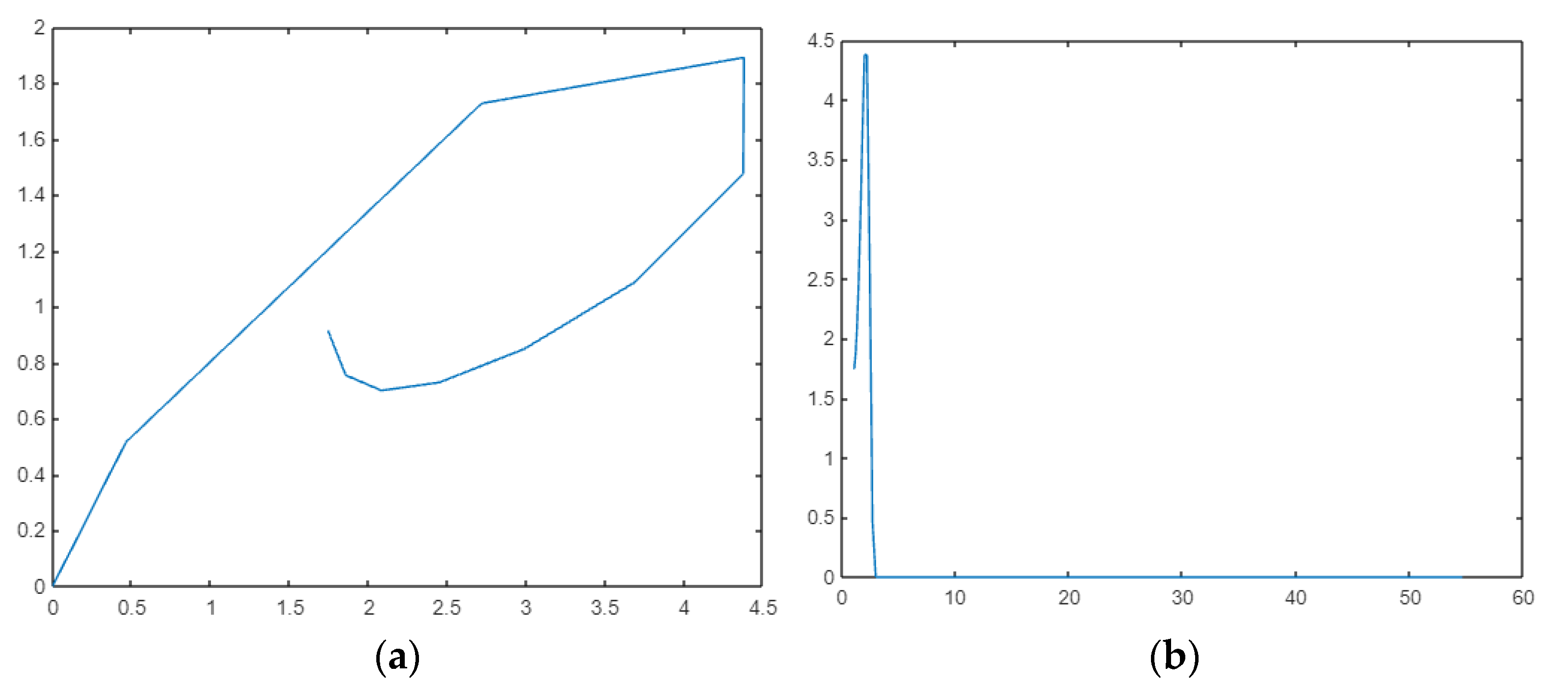
Moreover, the graph of the cancerous cell population with respect to time is sketched in Figure 1. We set initial values and constants according to the previous discussion, and the cell population is stored in the vectors B and C. Since Equation (1) is autonomous, we can rewrite that system of ODE into one single equation. Consequently, we have an ODE that is based on the derivative of healthy cells in terms of cancerous cells. The phase diagram in this case shows the population of one species with respect to another one.

5. Discussion

We introduced a model based on bi-geometric calculus, a kind of non-Newtonian calculus. This new interpretation of the population model gives insight into the description of the real phenomena in the new dialogue. This approach leads to the Hadamard fractional differential equation, whose existence and uniqueness are debated. The numerical method is extended and generalized to fit the corresponding system. Many different models have been introduced before to describe the dynamic system, but our model is based on different aspects of debates. The results can be compared to previous models in which Newtonian calculus was used extensively. In this paper, we introduced different operators of non-Newtonian calculus, and each has specific properties with interesting attitudes. Further work can be dedicated to making different models based on different calculi.