
On the Equivalence between Integer- and Fractional Order-Models of Continuous-Time and Discrete-Time ARMA Systems


Abstract
:1. Introduction
- We work always on the sets of reals, , and integers, .
- All the ARMA systems, continuous-time or discrete-time, are considered as time-invariant, meaning that the corresponding equations are defined by constant parameters.
- We used the bilateral Laplace transform (LT) [13]:where is any real or complex function/distribution defined on and is its transform, provided it has a non-void region of convergence (ROC)
- The Fourier transform (FT) is obtained from the LT through the substitution with .
- The standard convolution is given by
- The Z transform (ZT) is defined bywhere is any discrete-time signal and .
- With the substitution, we obtain the discrete-time Fourier transform.
2. Background
2.1. Classic ARMA Models
2.2. The Problem
- The differential equation by a difference equation;
- The TF by pole-zero mapping techniques;
- The TF by the zero-order hold-equivalence technique;
- The system response by a covariance equivalence technique.
2.3. Signal Framework
- Deterministic signals that we will assume are bounded piecewise continuous or tempered distributions [45]. Besides, they are:
- (a)
- Exponential-order signals that have Laplace or Z transforms.In the CT case, these signals are assumed to be synthesized through the Bromwich integral (inverse Laplace transform):where is the LT of , is the abscissa of a vertical straight line inside the corresponding region of convergence, and .In the DT case, the signals are obtained with the Cauchy integral, inverse Z transform:where is the ZT and is a circle inside the corresponding region of convergence.With this class of signals, we can define the TF of a given system.
- (b)
- Signals absolutely or square integrable (summable) that have a Fourier transform. We may include periodic signals.These signals are synthesized by the CT and DT inverse Fourier transforms given by:where is the CT Fourier transform of , andwhere is the DT Fourier transform.With this class of signals, we can obtain the frequency response of any linear system.
- Stochastic processesLet , be a zero-mean, second-order stationary process with the power spectral density function (PSD) . For each realization of the process, we can introduce a Crámer spectral representation [46] that assumes the formin the CT case. Similarly, for the DT case, we have [35,46]In each case, is an orthogonal stochastic process with and The operator stands for the expected value. As in the deterministic case, with this class of signals, we can obtain the frequency response of any linear system. To show it, we insert (12) into (14) and define the frequency response as the FT of the impulse response.
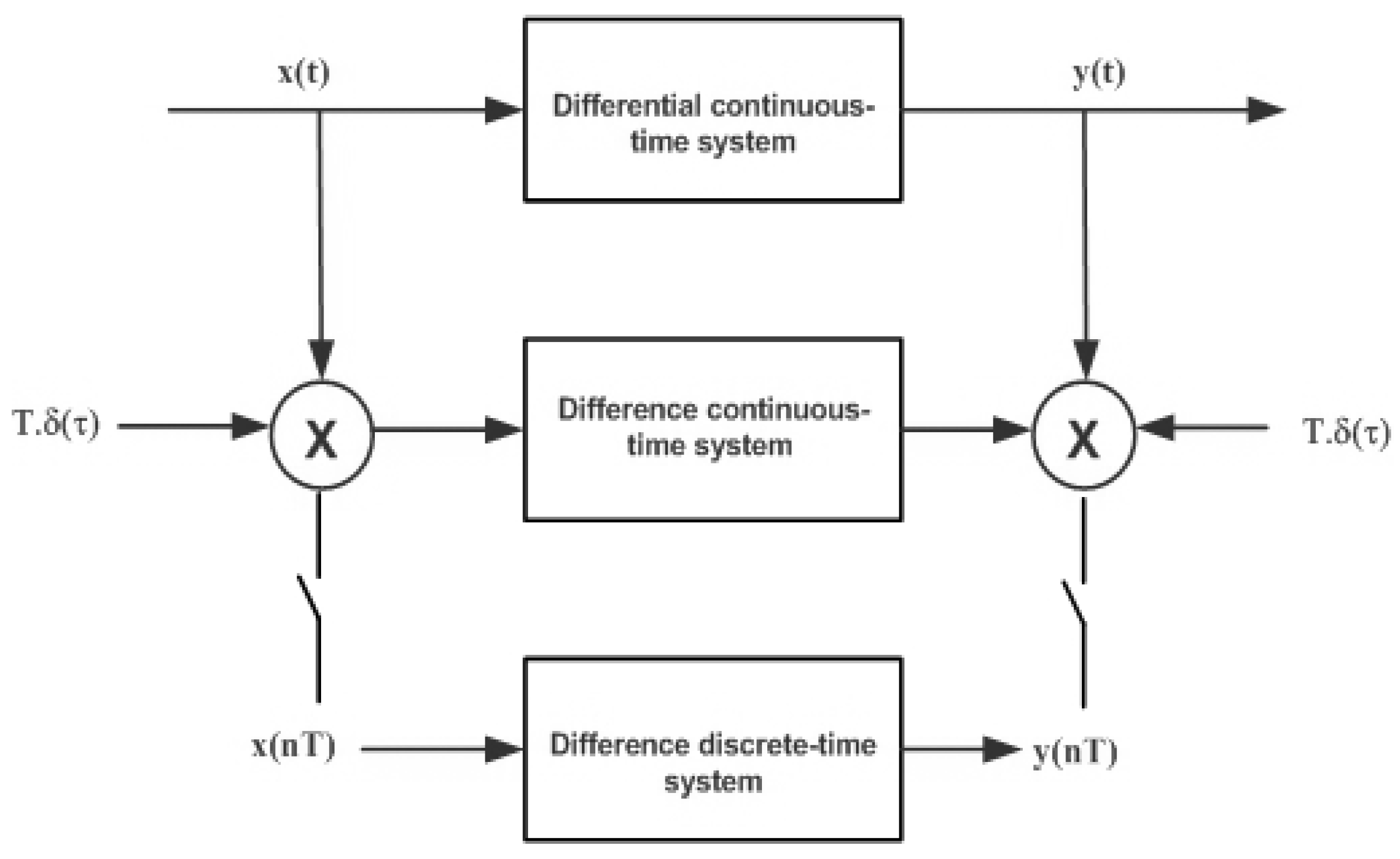
2.4. Equivalent Systems
- Is there any discrete-time linear system that gives as the output when the input is ?
- If it exists, which is its TF, ?
- Is there any relation between the transfer functions of the continuous- and discrete-time systems?
- Can we use the parameters of the discrete-time system to identify the continuous-time system?
- Is there any continuous-time linear system that relates the interpolated signals and ?
- If it exists, which is its TF, ?
- Is there any relation between the transfer functions of the continuous- and discrete-time systems?
- How can we compute the TF from ?
3. From Continuous-Time to Discrete-Time in Integer-Order Systems
3.1. Generalities
3.2. Sampling
3.3. The “Sampled” System
- Using (14),and so, there is a relation between and :that is the discrete-time convolution (The factor T may seem useless in several expressions. It serves to give coherence to the formulae and to allow the recovery of the continuous formulation when T goes to zero.).
- The function is a discrete-time signal resulting from the sampling of the impulse response of the system (7). Therefore, there is a TF, , of the “sampled system” such that and given by
- The eigenvalue corresponding to the eigenfunction is
3.4. A Continuous-Time Difference Equation
3.5. Non-Ideal Sampling and Interpolation
3.6. Discrete-Time Difference Equations
- The pole transformation is one-to-one ;
- The stability is preserved;
- The zeros are not preserved, because the new ones depend also on the poles;
- If , the sampled ARMA model we obtain has in general zeroes. Attending to (30), the system with only one pole is transformed into a system with also a zero.
3.7. Conversion Rules For Equivalence
3.7.1. Continuous To Discrete
- Simple poles:
- Double poles:
- Triple poles:
- For higher-order poles, we can obtain similar formulae by successive derivation. However, the above expressions suggest a general formulation:where numbers (see the “On-Line Encyclopedia of Integer Sequences ”: https://oeis.org/, accessed on 28 January 2022) are given by
- There is a one-to-one correspondence between the original poles and the poles of the discrete system;
- The stability is preserved, since gives ;
- The zeros are not preserved. The new zeros depend on the original, but also on the poles. To see this, consider a simple example . The corresponding discrete system is:
3.7.2. Discrete to Continuous
- Simple poles:If all the poles in (35) have order one, the sum of the residues is null and we can forget the constant term ().
- Second order poles
- Third-order poles:
- In the fourth order, we have
- The fifth order is
- In a matrix formulation, we can writeA general formula remains to be found.
3.8. Consequences
- Identifiability of continuous-time systems:We can identify a continuous-time system using the following procedure:
- (a)
- Sample input and output signals;
- (b)
- Compute the impulse response or directly the TF of the equivalent discrete system;
- (c)
- Obtain the partial fraction decomposition of the TF;
- (d)
- Using the conversion formulae, compute the TF of the continuous system;
- (e)
- From the TF, obtain the differential equation.
- Design of discrete-time systems from continuous-time templates:The design of continuous-time systems is a very well-studied and established theme with many methods existing, which have led to several templates. With these templates and using the above conversion formulae, we can obtain discrete-time equivalent systems. This procedure is exact and does not require a very small sampling interval.
- EmbeddingWe can find always a continuous-time system equivalent to a given discrete-time one.
4. Covariance Equivalence
- Energy signals:A signal is an energy signal or type energy [17] if . In this case, we define the function:such that . We conclude that
- Power signals:There are signals with infinite energy, but that have finite mean power defined by . We call them power signals or signals-type power. In this case, we define the function:such that . With this function, we reobtain (59).
- Stationary stochastic processes:For this case, we could also use the last result, since stationary stochastic processes are power signals. However, we would need to assume that the process was ergodic. Either way, we introduce the autocovariance:and obtain (59) again. Here, we can have a problem: the process may have a non-zero average. This is equivalent to including an intercept term [37], . According to the results in Section 3.1, when the input is a constant, the corresponding output is given by . For now, we assume that the system does not have a pole at the origin (singular case).
- Non-stationary stochastic processes:Consider the more involved situation in which the autocovariance is defined byHowever, it is not difficult to obtainwhich is similar to (59) and has the same interpretation: there is a new (non-causal) linear system having the TF with input and output verifying the differential equation:where with and with .
- No poles on the imaginary axis:If the TF of the original system, , has no poles on the imaginary axis, is analytical on a vertical strip that includes such an axis. This means that the system described by (61) is a stable system and all the considerations made in Section 3.1 and Section 3.7 remain valid, in particular all the conversion rules are applied also.The stability is assured by the absolute integrability of the impulse response, .
- Poles on the imaginary axis:If has poles on the imaginary axis, then doubles the poles there. This is a singular case that was treated in [47]. The corresponding time response increases without bound. The system is unstable.
- The covariance equivalence implies the input–output equivalence;
- The input–output equivalence may not imply the covariance equivalence (we can have poles on the imaginary axis);
- The input–output equivalence and the covariance equivalence are the same if:
- There are no poles on the imaginary axis of the continuous-time system (on the unit circle in the discrete case);
- All the zeroes are in the left half plane (in the unit disk).
The covariance “loses the phase” of the system.
5. The Bilinear Transformation: A Spectral Equivalence
5.1. The s to z Conversion
- It transforms the whole left complex plane into the unit disk;
- It maps the imaginary axis on the unit circle;
- It allows a one-to-one transformation from pole to pole and from zero to zero;
- It has an interpretation in terms of the trapezoidal integration.
- The frequency warping that happens in going from the imaginary axis to the unit circle [4];
- The zero at .
- :The discrete TF we obtain with the bilinear transformation iswith the new pole located atWe conclude that the new pole is at , but it should be at . We will study this change below for several values of p. Meanwhile, we must realize that the static gain does not change: . As above, a zero at appears.
- Now, we obtainwith .On the other hand, we have again
- If the continuous-time system is stable, the corresponding discrete-time one is also stable;
- If the continuous-time system is minimum phase, so is the corresponding discrete-time one—if zeros on the left half complex plane are transformed into zeros inside the unit circle, as is easy to see;
- The static gain is invariant;
- If the original system is an ARMA(N,M), the TF of the discrete-time system is an ARMA(N,N). This is clear from the above examples. We can see that the simple fractions without zero originate a zero at . Therefore, the corresponding spectrum is zero at . The zero at has order .
5.2. Spectral Equivalence
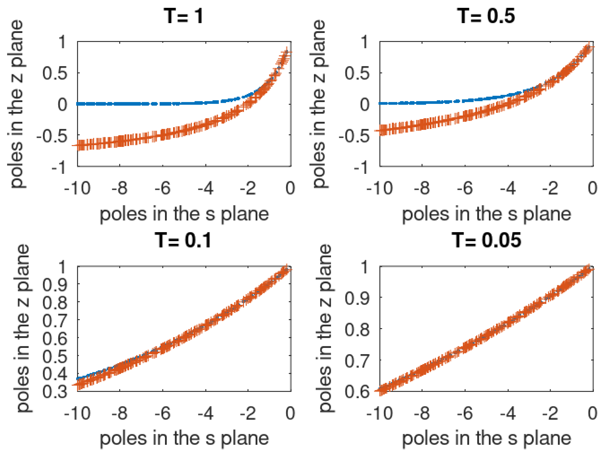
- Continuous to discrete:In this case, we can write from aboveWe can choose T as small as we can to obtainThis means that the bilinear equivalence can be assured, as we will see later, in the continuous to discrete conversion.In Figure 3, we illustrate the evolution of the transformed poles. We generated 200 negative real poles and applied the exponential and the binomial transformation for .
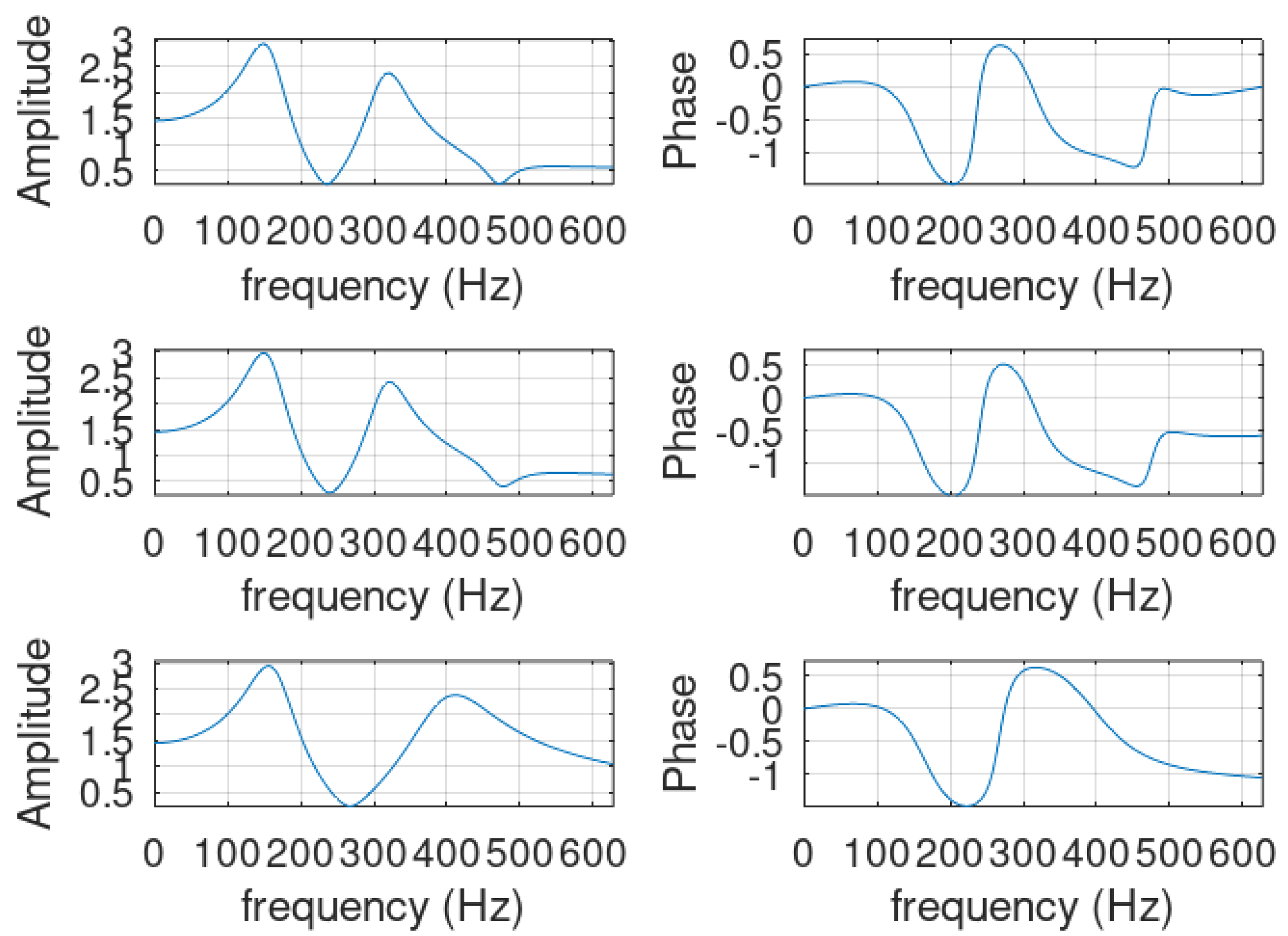
- Discrete to continuous:This situation is different from the above since the approximation does not depend on T. In fact, from (65), only if is small and which is independent of the sampling interval. This leads us to conclude that only the spectral components with a low frequency can remain undistorted when going from discrete to continuous. We will illustrate this situation later.
5.3. The FIR Systems
5.4. The Pole at
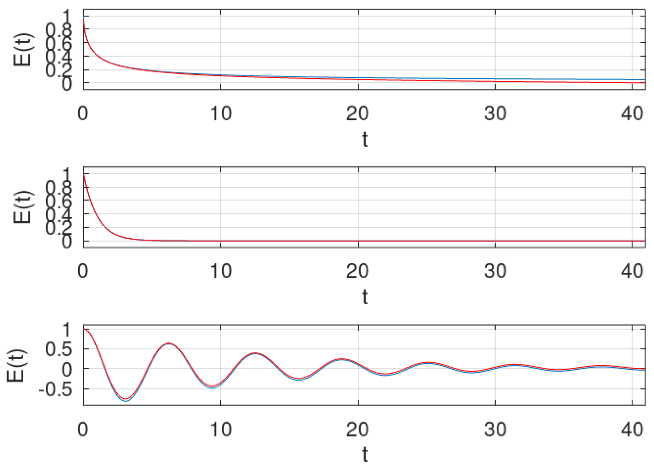
5.5. Simulation Results
6. From Continuous-Time to Discrete-Time in Fractional Systems
6.1. The Fractional Linear Systems
6.2. On the Fractional Discrete-Time Models
6.2.1. Euler Type Systems
- Many stable DT systems are outside the stability region implied by this derivative;
- We have to define a new DT Laplace transform [11], preventing the direct use of the Z transform and, consequently, the FFT.
6.2.2. Bilinear-Type Systems
6.3. The Bilinear Discrete-Time Linear Systems
6.4. Equivalence
7. Conclusions
Author Contributions
Funding
Data Availability Statement
Conflicts of Interest
Abbreviations
| ARMA | autoregressive-moving average |
| CT | continuous-time |
| DT | discrete-time |
| FARMA | fractional autoregressive-moving average |
| FT | Fourier transform |
| FFT | Fast Fourier transform |
| GL | Grünwald-Letnikov |
| LT | Laplace transform |
| TF | transfer function |
| ZT | Z transform |
References
- Kailath, T. Linear Systems; Information and System Sciences Series; Prentice-Hall: Hoboken, NJ, USA, 1980. [Google Scholar]
- Oppenheim, A.V.; Schafer, R.W. Digital Signal Processing; Prentice-Hall: Englewood Clifs, NJ, USA, 1975. [Google Scholar]
- Ortigueira, M.D.; Valério, D. Fractional Signals and Systems; De Gruyter: Berlin, Germany; Boston, MA, USA, 2020. [Google Scholar]
- Proakis, J.G.; Manolakis, D.G. Digital Signal Processing: Principles, Algorithms, and Applications; Prentice Hall: Hoboken, NJ, USA, 2007. [Google Scholar]
- Kirshner, H.; Unser, M.; Ward, J.P. On the Unique Identification of Continuous-Time Autoregressive Models From Sampled Data. IEEE Trans. Signal Process. 2014, 62, 1361–1376. [Google Scholar] [CrossRef]
- Box, G.E.P.; Jenkins, G.M. Time Series Analysis: Forecasting and Control; Holden Day: San Francisco, CA, USA, 1976. [Google Scholar]
- Ljung, L. System Identification: Theory for the User; Prentice-Hall: Englewood Cliffs, NJ, USA, 1999. [Google Scholar]
- Ortigueira, M.D. ARMA Realization from the Reflection Coefficient Sequence. Signal Process. 1993, 32, 329–342. [Google Scholar] [CrossRef]
- Pintelon, R.; Schoukens, J. System Identification: A Frequency Domain Approach; IEEE Press: New York, NY, USA, 2001. [Google Scholar]
- Ortigueira, M.D.; Machado, J.A.T. New discrete-time fractional derivatives based on the bilinear transformation: Definitions and properties. J. Adv. Res. 2020, 25, 1–10. [Google Scholar] [CrossRef]
- Ortigueira, M.D.; Coito, F.J.V.; Trujillo, J.J. Discrete-time differential systems. Signal Process. 2015, 107, 198–217. [Google Scholar] [CrossRef]
- Ortigueira, M.D.; Machado, J.A.T. The 21st century systems: An updated vision of discrete-time fractional models. IEEE Circuits Syst. Mag. 2022, 22. [Google Scholar] [CrossRef]
- Ortigueira, M.D.; Machado, J.A.T. A Review of Sample and Hold Systems and Design of a New Fractional Algorithm. Appl. Sci. 2020, 10, 7360. [Google Scholar] [CrossRef]
- Antoniou, A. Digital Signal Processing, 2nd ed.; Mcgraw-Hill: New York, NY, USA, 2016. [Google Scholar]
- Papoulis, A. Signal Analysis; McGraw-Hill Electrical and Electronic Engineering Series; McGraw-Hill: New York, NY, USA, 1977. [Google Scholar]
- DeCarlo, R.A. Linear Systems: A State Variable Approach with Numerical Implementation; Prentice-Hall, Inc.: Upper Saddle River, NJ, USA, 1989. [Google Scholar]
- Haykin, S.; Van Veen, B. Signals and Systems; John Wiley & Sons, Inc.: Hoboken, NJ, USA, 1999. [Google Scholar]
- Roberts, M.J. Signals and Systems: Analysis Using Transform Methods and Matlab; McGraw-Hill: New York, NY, USA, 2003. [Google Scholar]
- Marelli, D.; Fu, M. On the indirect approaches for CARMA model identification. Automatica 2007, 43, 1457–1463. [Google Scholar]
- Dorf, R.C.; Bishop, R.H. Modern Control Systems, 11th ed.; Pearson Prentice Hall: Hoboken, NJ, USA, 2008. [Google Scholar]
- Svoboda, J.A.; Dorf, R.C. Introduction to Electric Circuits; John Wiley & Sons: Hoboken, NJ, USA, 2013. [Google Scholar]
- Garnier, H.; Young, P.C. What does continuous-time model identification have to offer? IFAC Proc. Vol. 2012, 45, 810–815. [Google Scholar] [CrossRef] [Green Version]
- Brockwell, P.J. Representations of continuous-time ARMA processes. J. Appl. Probab. 2004, 41, 375–382. [Google Scholar] [CrossRef]
- Andersen, P.; Brincker, R.; Kirkegaard, P.H. Theory of Covariance Equivalent ARMAV Models. Civil Engineering Structures. In Proceedings of the 14th International Modal Analysis Conference (IMAC), Dearborn, MI, USA, 12–15 February 1996. [Google Scholar]
- Aström, K.J.; Hagander, P.; Sternby, J. Zeros of Sampled Systems. Automatica 1984, 20, 31–38. [Google Scholar] [CrossRef]
- Unbehauen, H.; Rao, G.P. A review of identification in continuous-time systems. Annu. Rev. Control 1998, 22, 145–171. [Google Scholar] [CrossRef]
- Brockwell, P.J. Recent results in the theory and applications of CARMA processes. Ann. Inst. Stat. Math. 2014, 66, 647–685. [Google Scholar] [CrossRef]
- Rao, G.P.; Unbehauen, H. Identification of Continuous-Time Systems. IEE Proc. Control Theory Appl. 2006, 153, 185–220. [Google Scholar] [CrossRef]
- Garnier, H.; Wang, L. Identification of Continuous-Time Models from Sampled Data; Springer: London, UK, 2008. [Google Scholar]
- Gillberg, J.; Ljung, L. Frequency-domain identification of continuous-time ARMA models from sampled data. Automatica 2009, 45, 1371–1378. [Google Scholar] [CrossRef] [Green Version]
- Kirshner, H.; Maggio, S.; Unser, M. A Sampling Theory Approach for Continuous ARMA Identification. IEEE Trans. Signal Process. 2011, 59, 4620–4644. [Google Scholar] [CrossRef] [Green Version]
- Marelli, D.; Fu, M. A Continuous-Time Linear System Identification Method for Slowly Sampled Data. IEEE Trans. Signal Process. 2010, 58, 2521–2533. [Google Scholar] [CrossRef]
- Marelli, D.; You, K.; Fu, M. Identification of ARMA models using intermittent and quantized output observations. Automatica 2013, 49, 360–369. [Google Scholar] [CrossRef]
- Pollock, D.S.G. The Correspondence Between Stochastic Linear Difference and Differential Equations. In International Conference on Time Series and Forecasting; Springer: Cham, Switzerland, 2019; pp. 31–49. [Google Scholar]
- Pollock, D.S.G. Linear Stochastic Models in Discrete and Continuous Time. Econometrics 2020, 8, 35. [Google Scholar] [CrossRef]
- Söderström, T.; Irshad, I.; Mossberg, M.; Zheng, W.X. On the accuracy of a covariance matching method for continuous-time errors-in-variables identification. Automatica 2013, 49, 2982–2993. [Google Scholar] [CrossRef]
- Thornton, M.A.; Chambers, M.J. Continuous-time autoregressive moving average processes in discrete time: Representation and embeddability. J. Time Ser. Anal. 2013, 34, 552–561. [Google Scholar] [CrossRef]
- Brockwell, A.E.; Brockwell, P.J. A Class of Non-Embeddable ARMA Processes. J. Time Ser. Anal. 1998, 20, 483–486. [Google Scholar] [CrossRef]
- Unser, M. Sampling-50 years after Shannon. Proc. IEEE 2000, 88, 569–587. [Google Scholar] [CrossRef] [Green Version]
- Arratia, A.; Cabaña, A.; Cabaña, E.M. Embedding in law of discrete time ARMA processes in continuous time stationary processes. J. Stat. Plan. Inference 2018, 197, 156–167. [Google Scholar] [CrossRef]
- Huzii, M. Embedding a Gaussian discrete-time autoregressive moving average process in a Gaussian continuous-time autoregressive moving average process. J. Time Ser. Anal. 2007, 28, 498–520. [Google Scholar] [CrossRef]
- Ortigueira, M.D. The comb signal and its Fourier Transform. Signal Process. 2001, 81, 581–592. [Google Scholar] [CrossRef] [Green Version]
- Kwakernaak, H.; Sivan, R. Modern Signals and Systems; Prentice-Hall, Inc.: Hoboken, NJ, USA, 1991. [Google Scholar]
- Mossberg, M. Estimation of continuous-time stochastic signals from sample covariances. IEEE Trans. Signal Process. 2008, 56, 821–825. [Google Scholar] [CrossRef]
- Zemanian, A.H. Distribution Theory and Transform Analysis; Dover Publications: New York, NY, USA, 1987. [Google Scholar]
- Priestley, M.B. Spectral Analysis and Time Series; Academic Press: London, UK, 1981. [Google Scholar]
- Ortigueira, M.D. On the particular solution of constant coefficient ordinary differential equations. Appl. Math. Comput. 2014, 232, 254–260. [Google Scholar]
- Ferreira, J.C. Introduction to the Theory of Distributions; Pitman Publ.: Dordrecht, The Netherlands, 1997. [Google Scholar]
- Braslavsky, J.; Meinsma, G.; Middleton, R.; Freudenberg, J. On a key sampling formula relating the Laplace and Z transforms. Syst. Control Lett. 1997, 29, 181–190. [Google Scholar] [CrossRef]
- Henrici, P. Applied Computational Complex Analysis; Wiley-Interscince Publication: Hoboken, NJ, USA, 1974; Volume 1. [Google Scholar]
- Gonçalves, E. Une généralisation des processus ARMA. Annales d’Economie Statistique 1987, 109–145. [Google Scholar] [CrossRef]
- Pollock, D.S.G. (Ed.) Handbook of Time Series Analysis, Signal Processing, and Dynamics; Academic Press: London, UK, 1999. [Google Scholar]
- Ortigueira, M.D. Introduction to fractional linear systems. Part 2. Discrete-time case. IEE Proc. Vision Image Signal Process. 2000, 147, 71–78. [Google Scholar] [CrossRef] [Green Version]
- Ortigueira, M.D.; Machado, J.A.T. The 21st century systems: An updated vision of continuous-time fractional models. IEEE Circuits Syst. Mag. 2022, 22. [Google Scholar] [CrossRef]
- Doukhan, P. Stochastic Models for Time Series; Springer: Berlin, Germany, 2018; Volume 80. [Google Scholar]
- Tustin, A. A method of analysing the behavior of linear systems in terms of time series. J. Inst. Electr. Eng. Part IIA Autom. Regul. Servo Mech. 1947, 94, 130–142. Available online: https://digital-library.theiet.org/content/journals/10.1049/ji-2a.1947.0020 (accessed on 28 January 2022).
- Magin, R.; Ortigueira, M.D.; Podlubny, I.; Trujillo, J. On the fractional signals and systems. Signal Process. 2011, 91, 350–371. [Google Scholar] [CrossRef]
- Ortigueira, M.D. Fractional Calculus for Scientists and Engineers; Lecture Notes in Electrical Engineering, 84; Springer: Dordrecht, The Netherlands, 2011. [Google Scholar]
- Gorenflo, R.; Kilbas, A.A.; Mainardi, F.; Rogosin, S.V. Mittag-Leffler Functions, Related Topics and Applications; Springer Monographs in Mathematics; Springer: Berlin/Heidelberg, Germany, 2014. [Google Scholar]
- Ortigueira, M.D.; Lopes, A.M.; Machado, J.A.T. On the numerical computation of the Mittag-Leffler function. Int. J. Nonlinear Sci. Numer. Simul. 2019, 20, 725–736. [Google Scholar] [CrossRef]
- Ortigueira, M.D.; Bengochea, G.; Machado, J.A.T. Substantial, tempered, and shifted fractional derivatives: Three faces of a tetrahedron. Math. Methods Appl. Sci. 2021, 44, 9191–9209. [Google Scholar] [CrossRef]
- Ortigueira, M.D. Two-sided and regularised Riesz-Feller derivatives. Math. Methods Appl. Sci. 2021, 44, 8057–8069. [Google Scholar] [CrossRef]
- Ortigueira, M.D.; Bengochea, G. Bilateral Tempered Fractional Derivatives. Symmetry 2021, 13, 823. [Google Scholar] [CrossRef]


| T | |||
|---|---|---|---|
| Max-abs | |||
| Min-abs | |||
| Max-angle |
Publisher’s Note: MDPI stays neutral with regard to jurisdictional claims in published maps and institutional affiliations. |
© 2022 by the authors. Licensee MDPI, Basel, Switzerland. This article is an open access article distributed under the terms and conditions of the Creative Commons Attribution (CC BY) license (https://creativecommons.org/licenses/by/4.0/).
Share and Cite
Ortigueira, M.D.; Magin, R.L. On the Equivalence between Integer- and Fractional Order-Models of Continuous-Time and Discrete-Time ARMA Systems. Fractal Fract. 2022, 6, 242. https://doi.org/10.3390/fractalfract6050242
Ortigueira MD, Magin RL. On the Equivalence between Integer- and Fractional Order-Models of Continuous-Time and Discrete-Time ARMA Systems. Fractal and Fractional. 2022; 6(5):242. https://doi.org/10.3390/fractalfract6050242
Chicago/Turabian StyleOrtigueira, Manuel Duarte, and Richard L. Magin. 2022. "On the Equivalence between Integer- and Fractional Order-Models of Continuous-Time and Discrete-Time ARMA Systems" Fractal and Fractional 6, no. 5: 242. https://doi.org/10.3390/fractalfract6050242