1. Introduction
Infectious diseases, especially the outbreak and pandemic of emerging infectious diseases, have become a major public health problem around the world. Neither modern science nor technology can predict when and where a new infection will occur. However, once this occurs, it is often not possible to respond in a timely and effective manner due to a lack of understanding of the epidemic. For example, COVID-19, at the end of 2019, with its high infection rate and rapid onset of the cycle, has posed a huge threat to human lives and caused immeasurable losses to the economy of China and even the entire world. Therefore, the study of pathogenesis, the law of transmission, as well as strategies for the prevention and treatment of infectious diseases are of great practical importance and perspective.
The network model is one of the most widely studied models in recent years. Individuals in a crowd are treated as nodes in the network, and the relationship between individuals is described by edges between the nodes. The most influential research was carried out by Pastor-Satorras and Vespignani in [
1], where SIS (susceptible-infected-susceptible) and SIR (susceptible-infected-recovered) models were studied using mean field theory. Moreover, in order to better analyze the characteristics of disease transmission in the population, not only the evolution of the population network was taken into account but also the transmission of information about the disease. Recently, some researchers [
2,
3,
4,
5] have extended the dynamics of transmission of infectious disease to a multi-layer network, which led to a deeper study of mathematical epidemiology. Kan et al. [
6] introduced a self-consciousness variable and found that the infection threshold and the infected density are influenced by the consciousness network, the topology of the disease network, and the effective transmission rate. In addition, some scientists proposed a transmission model of infectious diseases in a multi-layer coupling network from a new perspective in [
7,
8,
9]. The transmission probability among the set of possible node states and the influence of network topology on the transmission threshold were analyzed in a multi-layer network. In [
10], the awareness of infection risk was incorporated into the Volz–Miller SIR epidemic model, to study the effect of awareness on disease dynamics.
As the above research progressed, it became clear that the strength of the relationship between people can seriously affect the transmission of the epidemic. Edge weights indicate the familiarity or intimacy of interactive individuals. The larger the weight of the edge between two nodes is, the easier the susceptible can be infected and the quicker the unknown individual can acquire the disease message. In [
11,
12,
13,
14], some methods for estimating disease transmission along the edges in weighted networks were presented. A modified epidemic SIS model with a birth–death process and nonlinear infectivity in an adaptive and weighted contact network was proposed in [
15]. The model indicated that the intimacy or familiarity between two related individuals would decrease as the disease progresses. To estimate the epidemic threshold and epidemic size on networks with general degree and weight distributions, a new edge-weight-based compartmental approach was developed in [
16]. It was found in [
17] that the weight exponent can contribute to the transmission of the epidemic by increasing the basic reproduction number, and the effect of the internal rate of infectiousness on the prevalence of the epidemic was greater than the effect of the rate of cross-infection for various network structures.
It can be found that the weight of the network has a great influence on the spread of disease. However, these studies did not put forward a control strategy to control the disease from the perspective of network weights. Therefore, in order for the transmission process to represent a realistic system, in this paper, we build a model of the epidemic on a weighted two-layer network and evaluate the impact of network weights on disease transmission, and try to propose an effective control method based on the network weights.
Since the fractional-order epidemic model is an extension of the integer-order epidemic model and it is more advantageous to describe processes that have memory and heritability, many scientists [
18,
19,
20] have used fractional order differential equations to analyze the dynamics of transmission of infectious diseases. Based on the basic reproduction number and Lyapunov’s theory of stability, Zafar et al. [
21] analyzed the stability of the equilibrium point of a fractional-order HIV/AIDS model and the control of its spread. Rostamy et al. [
22] discussed the existence of multiple equilibrium points in the SIR model and showed that choosing appropriate fractional order parameters can extend the stable region of the equilibrium points. In [
23], a mathematical model consisting of a system of nonlinear fractional order differential equations was presented, in which bats were considered as the origin of the virus that spread the disease into the human population. A fractional-order SIR model, which employs the Caputo fractional derivative and incorporates infectious and noninfectious abandonment dynamics, was discussed in [
24]. Furthermore, fractional-order SIR systems in the context of COVID-19 were built [
25,
26], especially, a novel modified predictor-corrector method was proposed to capture the nature of the obtained solution for a suitable nonlinear fractional dynamical system with different arbitrary orders [
27]. However, few studies [
28,
29] have analyzed the specific influence of fractional order on transmission dynamics. Therefore, quantifying the effect of fractional order on the transmission threshold for a specific model is a significant supplement to the dynamics of infectious diseases.
In addition, for fractional-order infectious disease models, some researchers have proposed vaccination control strategies to prevent the spread of the disease. If the immunity control objects are different, the control effect will be different. Age-targeted immunity [
30,
31], internet-information-driven immunity [
32,
33,
34], and dynamic immunity of human behavior [
35] are common control methods. A few studies [
36,
37,
38] have shown that people with low immunity are more likely to be infected and are less treatable. From the perspective of a complex network, people with low immunity are the nodes with low weights in the network. Therefore, the implementation of vaccination control for the nodes whose weight is less than a certain threshold can play a great role in controlling the spread of infectious diseases. Based on the fractional-order epidemic model on a two-layer weighted network, a targeted immunity control strategy is proposed for nodes whose weight is less than a certain value, which can not only suppress the spread of the epidemics but also save the cost of control.
The paper is organized as follows. In
Section 2, we propose a fractional-order SIR model for two-layer weighted networks. In
Section 3, the stability of the disease-free equilibrium and endemic equilibrium on weighted networks are analyzed separately. In
Section 4, a linear vaccine control based on age structure is presented to inoculate the nodes whose weights are less than a certain value. Numerical confirmation of the theoretical predictions is provided in
Section 5. Some conclusions are made in
Section 6.
2. Model Description
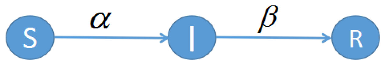
The nodes of the disease network can be divided into three categories: susceptible nodes S, infected nodes I, and recovery nodes R. The law of transmission is shown in
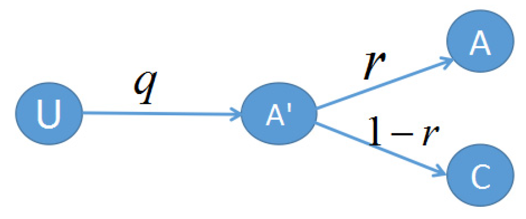
Figure 1. Social network nodes can also be divided into three categories: A represents the nodes that know the disease message and spread it out, C represents the nodes that know the disease message but do not spread it; U represents the nodes that do not know the disease message. The law of transmission between them is shown in
Figure 2.
In a social network for a node with the degree , its connection weight with node is . If node is connected with node , then ; on the contrary, then . Here, we will only focus on undirected networks, namely . According to previous research, the weight of nodes has a strong influence on disease transmission.
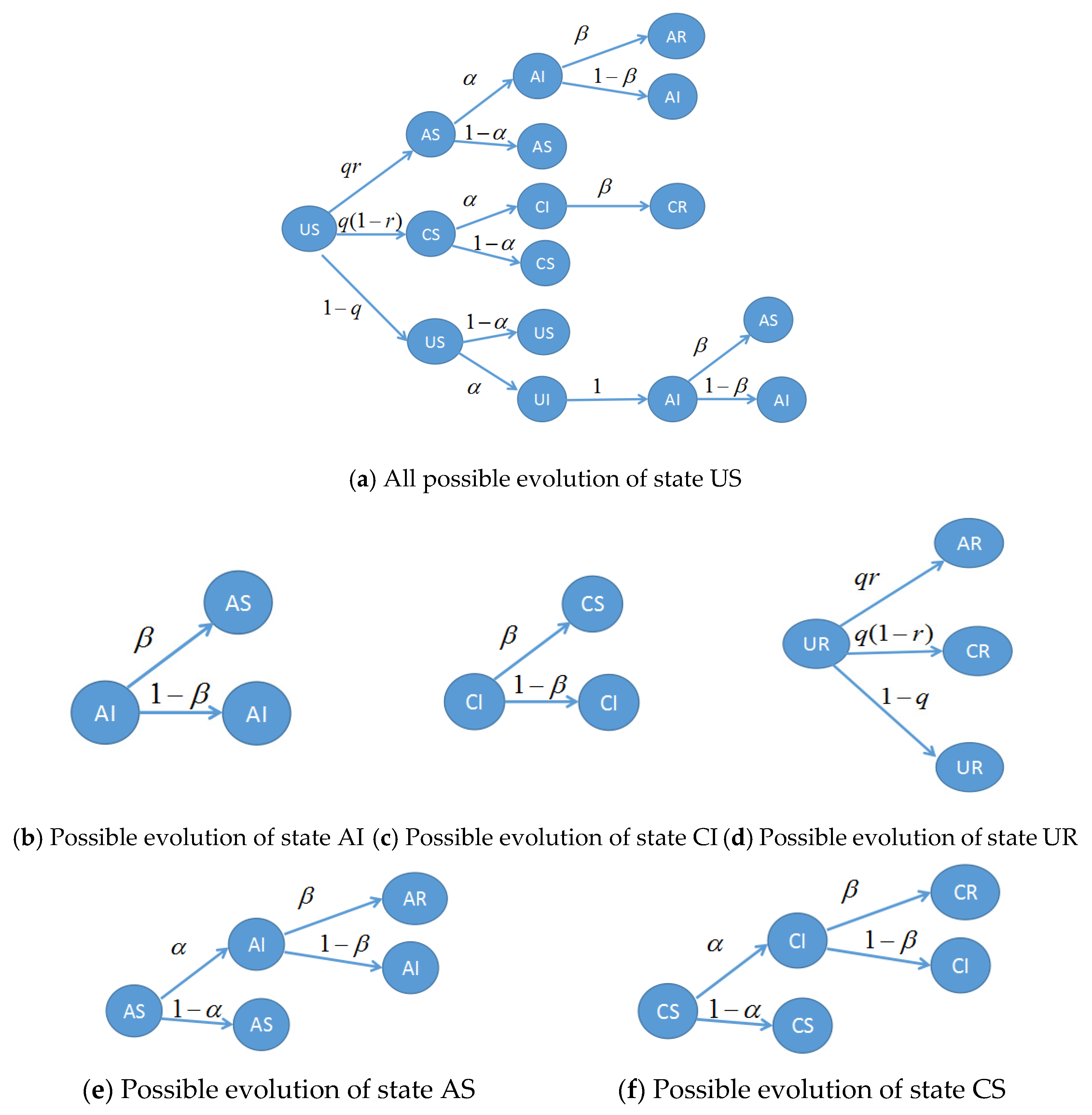
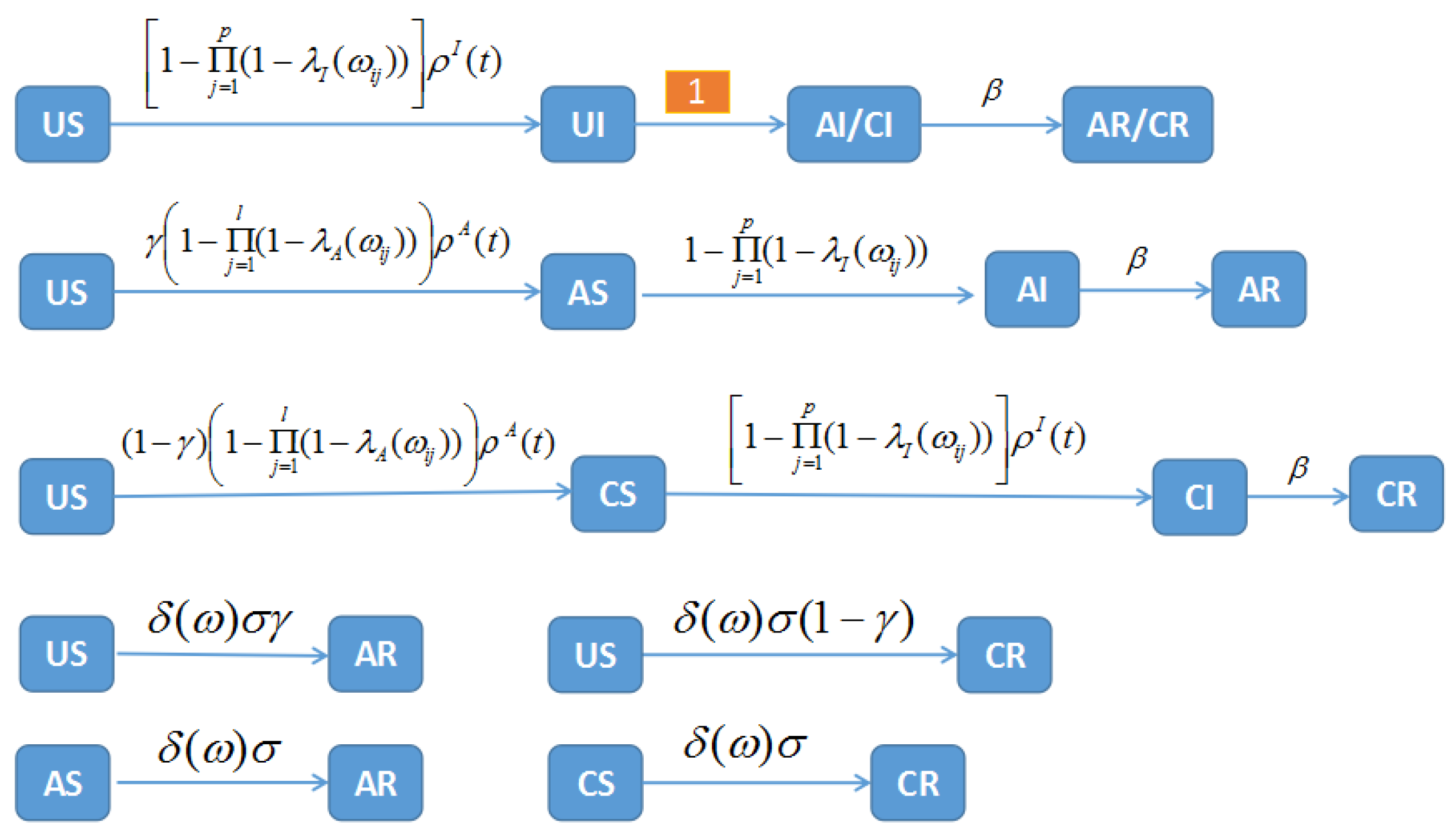
By combining the states of nodes in a social-disease network, all nodes can be divided into the following states: US, UR, AS, AI, AR, CS, CI, and CR. The law of transmission between states is shown in
Figure 3.
From
Figure 3, we can find that for a susceptible node
, the probability of its infection by the neighboring infected nodes is equal to
, based on the weight (the weight is determined by the social network). If there are
infected nodes with degree
, then the overall probability of infection is
. Likewise, for a node
, which does not know the disease message, the probability that it will receive a disease message from a neighboring node is
. If the degree of the node is
, where there are
nodes that know and transmit a message about the disease to other people, then the total probability of receiving information is
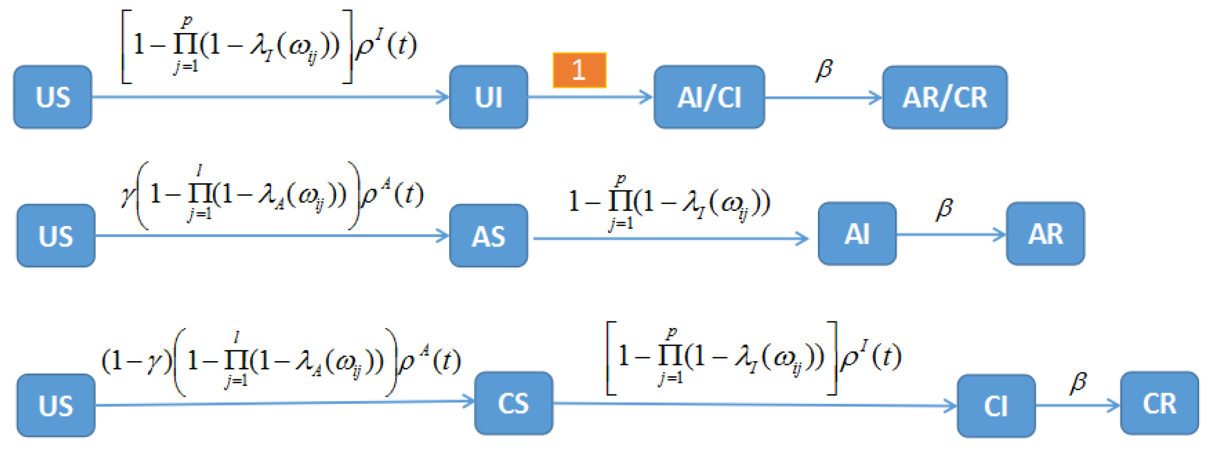
. Thus, the law of transmission between the eight states is shown in
Figure 4.
According to the relationship between disease transmission and information propagation, a fractional-order SIR network model in a two-layer network is established as follows:
where
is the Caputo differential with
,
is the density of the corresponding state at the time
. For example,
represents an infectious density at time
. The factor
represents the probability of infection of a node
in the disease network,
is the number of infected nodes in the neighboring nodes of a node
in the disease network. The factor
represents the probability of node
in the social network receiving a message,
is the number of nodes that know and distribute messages to the neighboring nodes of a node
in a social network.
Remark 1. If , then system (1) changes to an integer order system, which is the further generalization of the models proposed in [2,7] since it contains more possibilities for node states. Compared with the fractional-order models in [21,22,23,24], it not only considers the transmission of information between people but also considers the impact of the closeness of the connection between people on the transmission of information, e.g., the network weight. Therefore, the proposed model in this paper is more realistic and has practical significance. 3. Stability Analysis
Let
and
, then system (1) can be rewritten as follows:
For system (2), the Jacobian matrix
at equilibrium has the form
with
3.1. The Disease-Free Equilibrium
Let the right side of Equation (1) be equal to zero, then from (1a) and (1b) we can obtain that
From Equation (3), if , then and , and the disease-free equilibrium is .
If
, then
and
, and the disease-free equilibrium is
Firstly, we will analyze the stability of disease-free equilibrium .
When the disease-free equilibrium is
, the Jacobian matrix
is simplified to
The eigenvalues
of the matrix
can be calculated as follows:
It is easy to judge that
,
and
are all negative. If
then the system is unstable at equilibrium
.
Suppose , for matrix , the minimal polynomial of could be simplified to
. Since , then , only has one zero root, that is to say, the system is locally stable at .
Suppose , similarly, we can deduce that the minimal polynomial only has one zero root, and the system is locally stable at .
Since
and
, if
then inequality
holds.
From inequality (4), we can obtain:
Since
,
, therefore, if
holds, all eigenvalues in the disease-free equilibrium
are no more than zero and we can conclude that the system is locally stable at
.
Based on the above analysis, we can obtain the following theorem.
Theorem 1. For node , if is satisfied, while is the weight between node and node , and is the number of infectious neighboring nodes of node , then system (1) is locally stable on disease-free equilibrium .
Secondly, we will analyze the stability of disease-free equilibrium .
When the disease-free equilibrium is
, the Jacobian matrix
is
At this point, the eigenvalues
of the matrix
can be calculated as follows:
Obviously, if , by the same method, all the eigenvalues at disease-free equilibrium are not more than zero, and the system (1) is locally stable.
However, if , then , then the system (1) at disease-free equilibrium is unstable.
3.2. The Endemic Equilibrium
Suppose there is an endemic equilibrium, then
should be satisfied. From (1a), (1c), (1d) and (1g), we can obtain that
,
,
and
In addition, from (1b) and (1e), we have or . If , then substituting it into equation (1h) we have , which contradicts the hypothesis. If , then substituting it into (1c) and (1d), we also have , which contradicts the hypothesis.
Thus, for system (1) there is no endemic equilibrium, and there is only a disease-free equilibrium.
4. Targeted Immunity Based on Age Structure
For the infants and the elderly, their immunity is relatively poor and their influence on their surroundings is relatively small, which is reflected in complex networks that these special nodes have a relatively small weight. Taking targeted immunization against these special nodes with a small weight is a very effective control method to suppress the spread of infectious diseases in a wide range. Based on this, we propose a step function
related to the node weight, which is described as follows:
where
is the sum of weights of node
,
is the degree of node
,
is the given threshold value of weight. When the weight of a node in the network is less than or equal to
, the node is vaccinated with probability
. At this time, the transformation relationship among states of the network node is shown in
Figure 5.
Thus, the fractional-order SIR network model (1) can be rewritten as follows:
Similarly, for model (5), the disease-free equilibrium is and .
For
, the Jacobian matrix
is
For node
i, when
and
, the Jacobian matrix
at
can be written as
and the eigenvalues
of the matrix
can be calculated as follows:
When
and
, the Jacobian matrix
can be rewritten as
and the eigenvalues
of the matrix
can be calculated as follows:
Therefore, applying the same method, system (2) is always locally stable at .
Moreover, for
, the Jacobian matrix
is
Thus, system (2) is also locally stable at .
In the same way, we can deduce that there is also no endemic equilibrium under targeted immunity based on age structure, either.
When
, we can obtain the eigenvalues of the Jacobian matrix
Thus, system (2) is also locally stable at .
Corollary 1. If the network weight is a constant, then system (2) is always local stable at the disease-free equilibrium point.
Remark 2. Compared with the theoretical results in [16,17], the results present that the infected density is affected by the network weights and the node degree. In this paper, if the basic reproduction number is less than 1, we can conclude that the degree of decay is also influenced by the network weights, and even more, the infectious density is gradually truncated to zero, eventually. This result further simplifies the propagation law of infectious disease under-weighted networks. 5. Examples and Simulations
In this section, numerical simulations are presented to illustrate the theoretical results mentioned above.
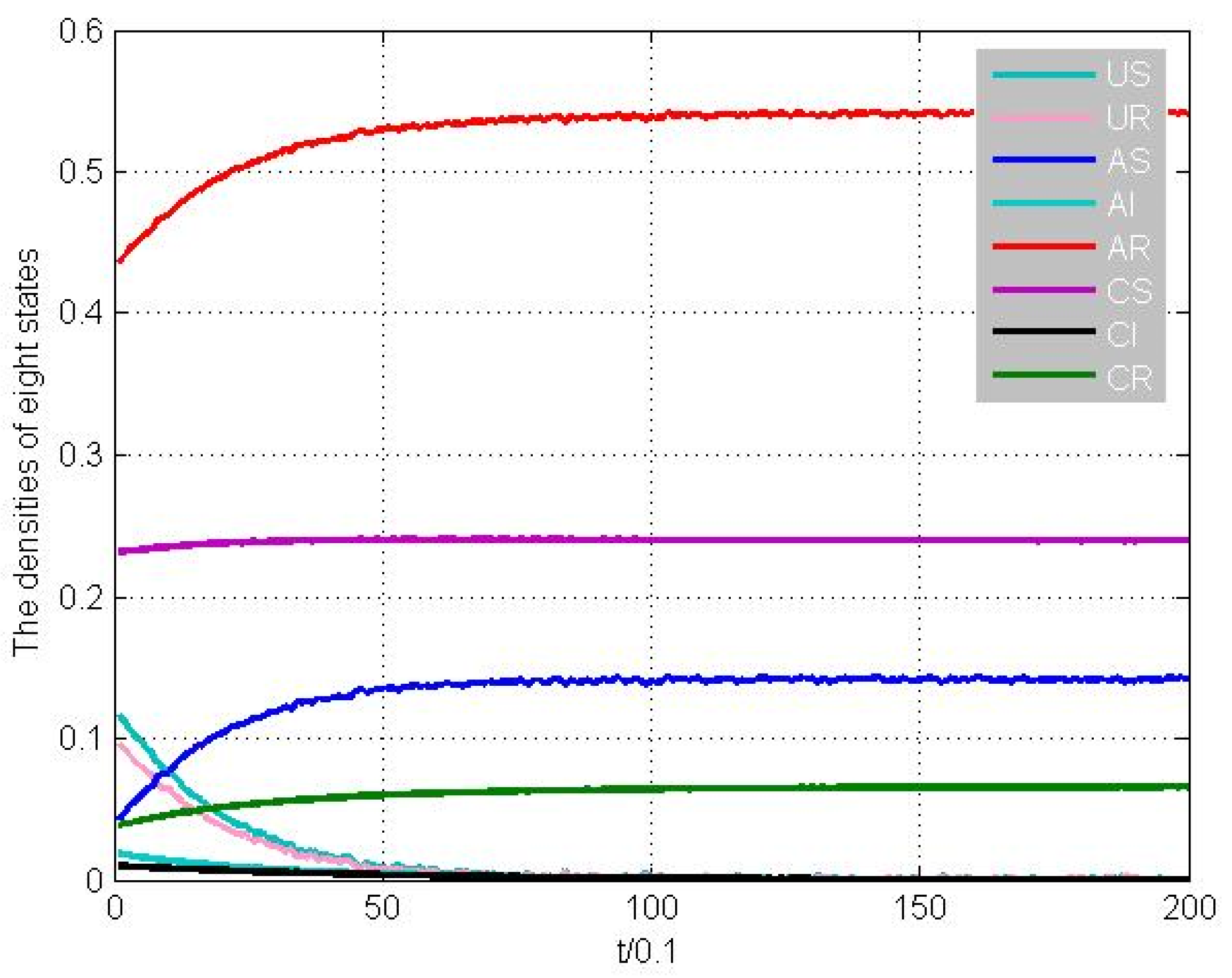
Example 1. Without loss of generality, for a node , suppose that , , , . The number of infectious neighboring nodes is equal , and the number of nodes that know and distribute messages is . The weights are valued as a random number between 0 and 1. The initial condition is [0.122, 0.1, 0.038, 0.019, 0.432, 0.231, 0.010, 0.038].
We can calculate that
and
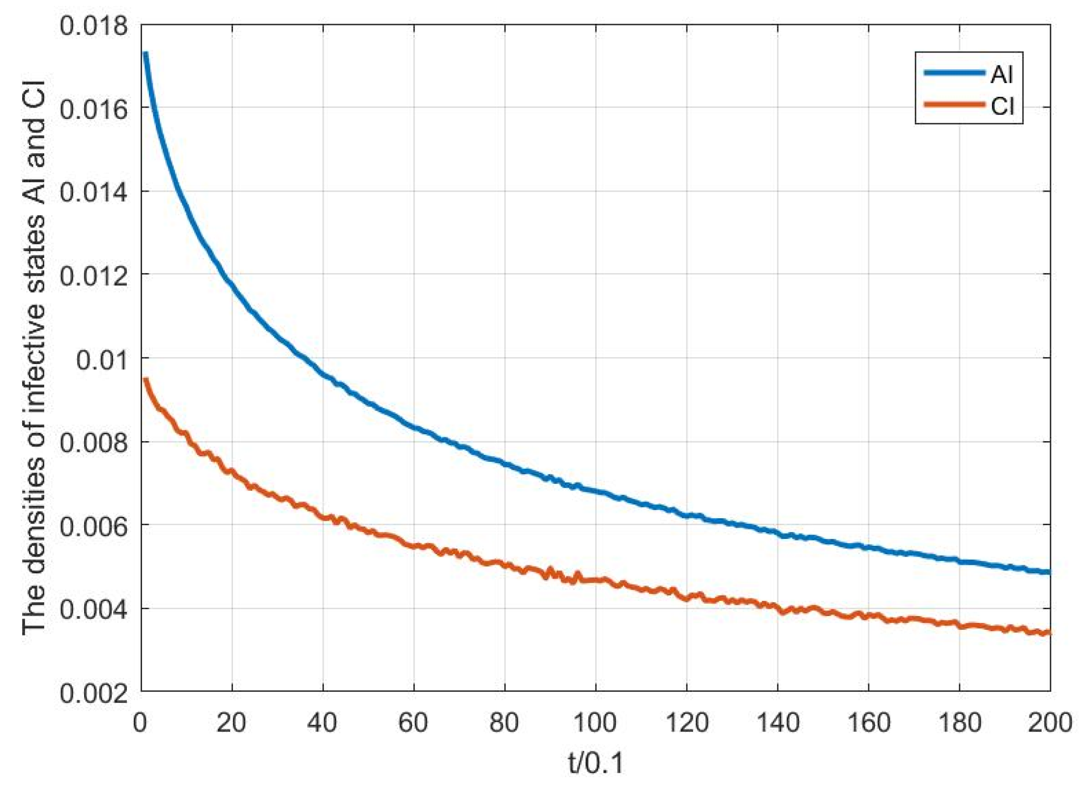
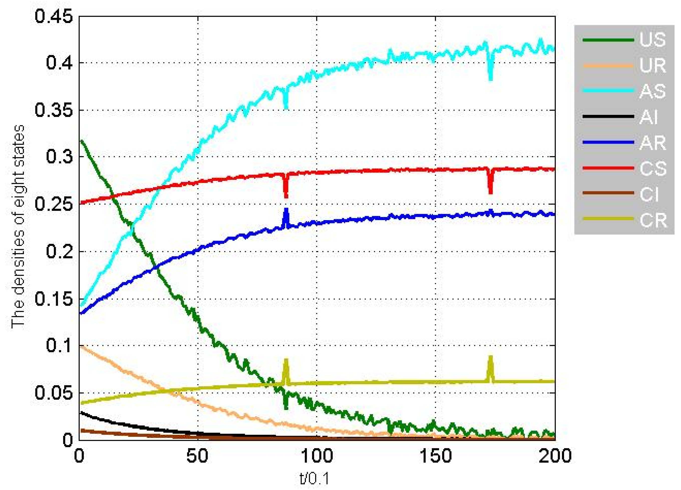
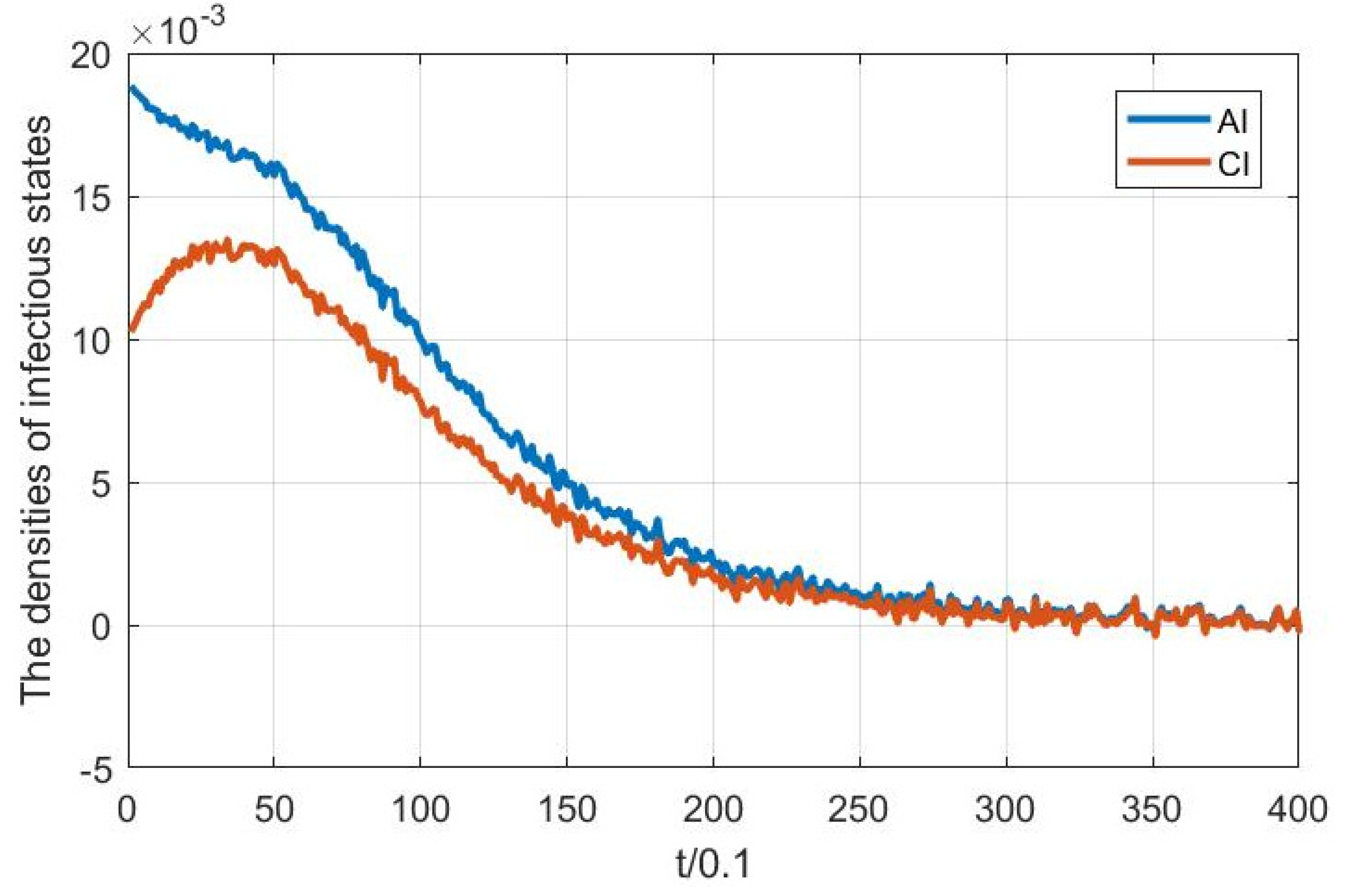
, which satisfies Theorem 1, thus there is only a disease-free equilibrium, and system (1) is locally stable. From
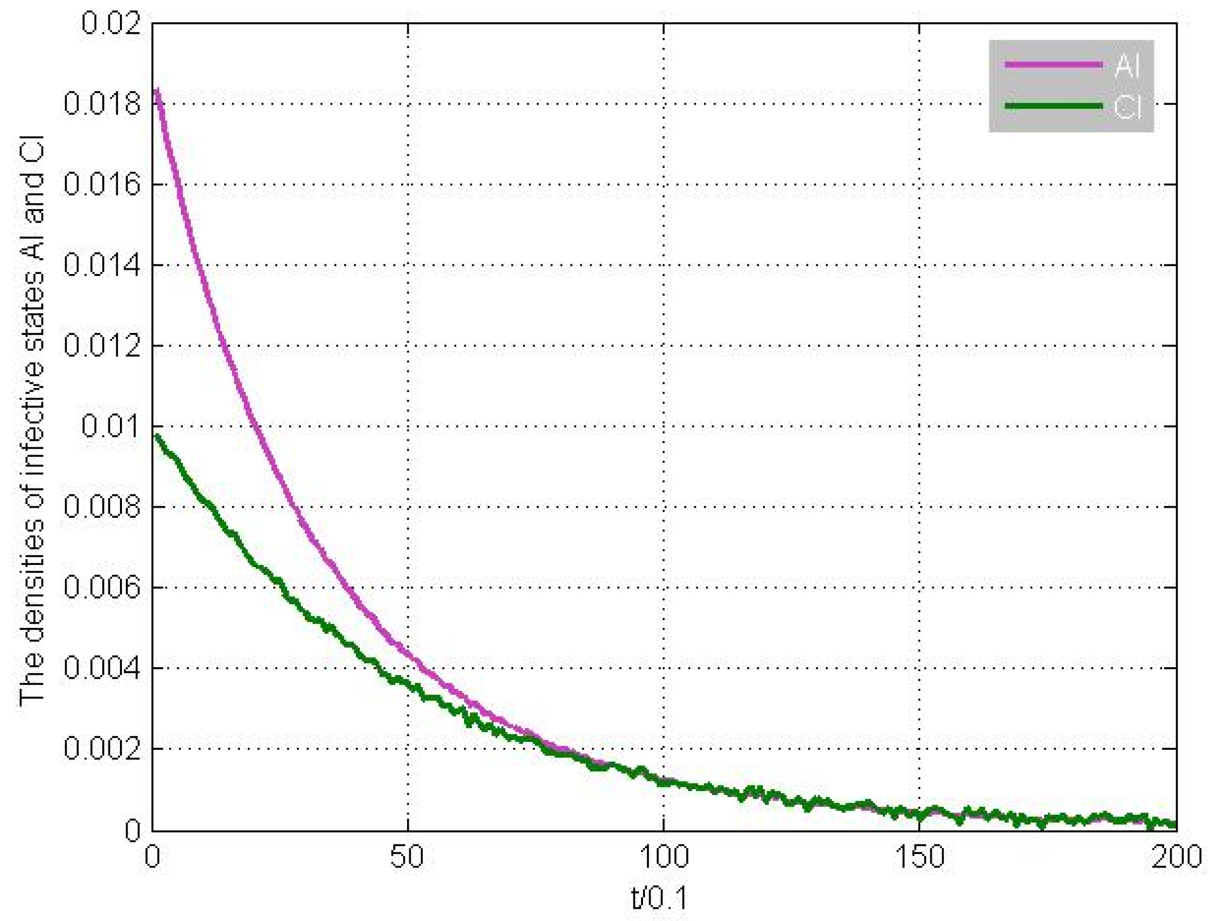
Figure 6, we can find that the disease-free equilibrium point is globally asymptotically stable. To be clear,
Figure 7 shows that the infectious states AI and CI converge to zero when
, which means that the disease will eventually disappear. From the above, we can conclude that the theoretical results are correct and the simulation results are effective.
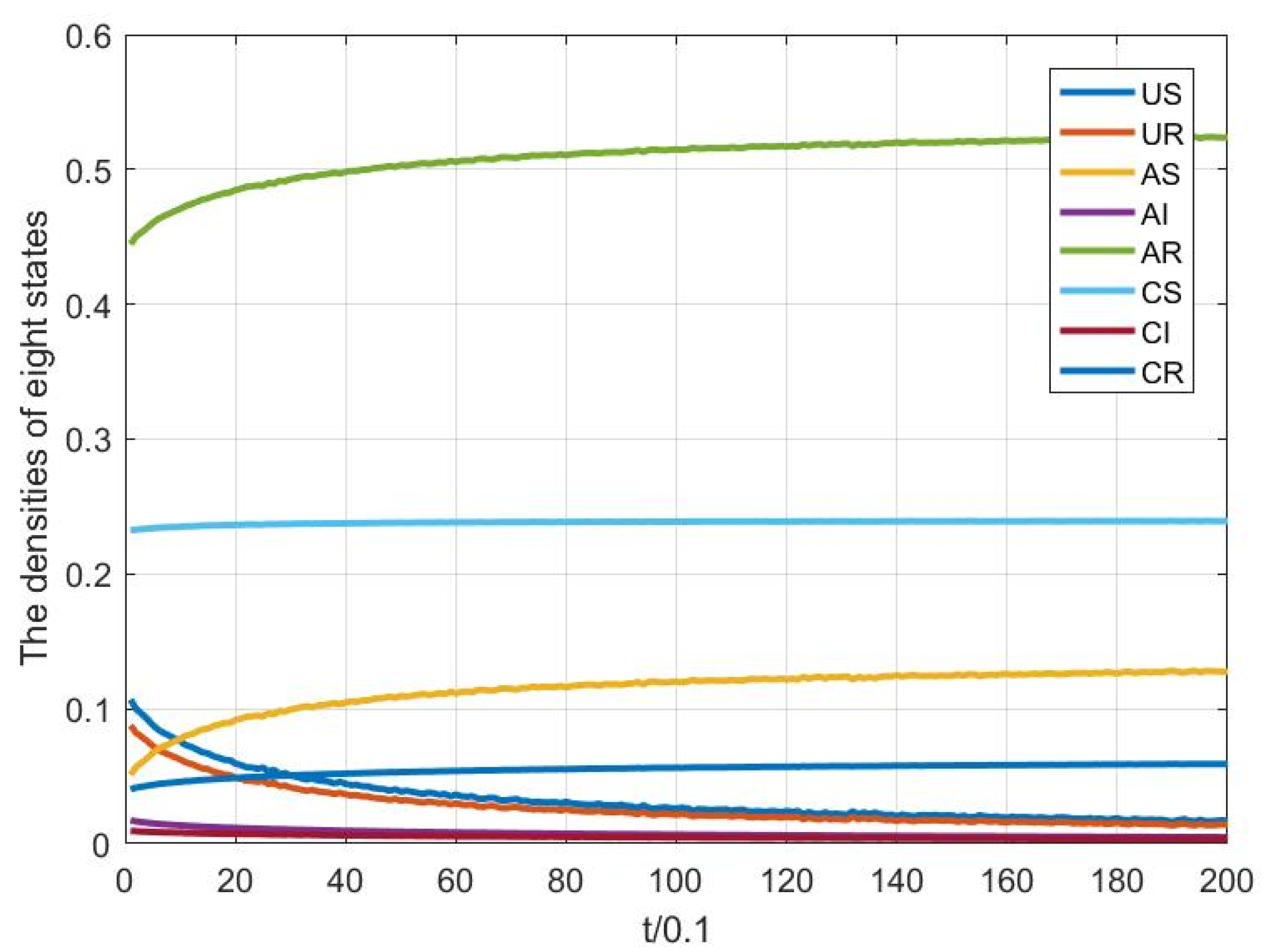
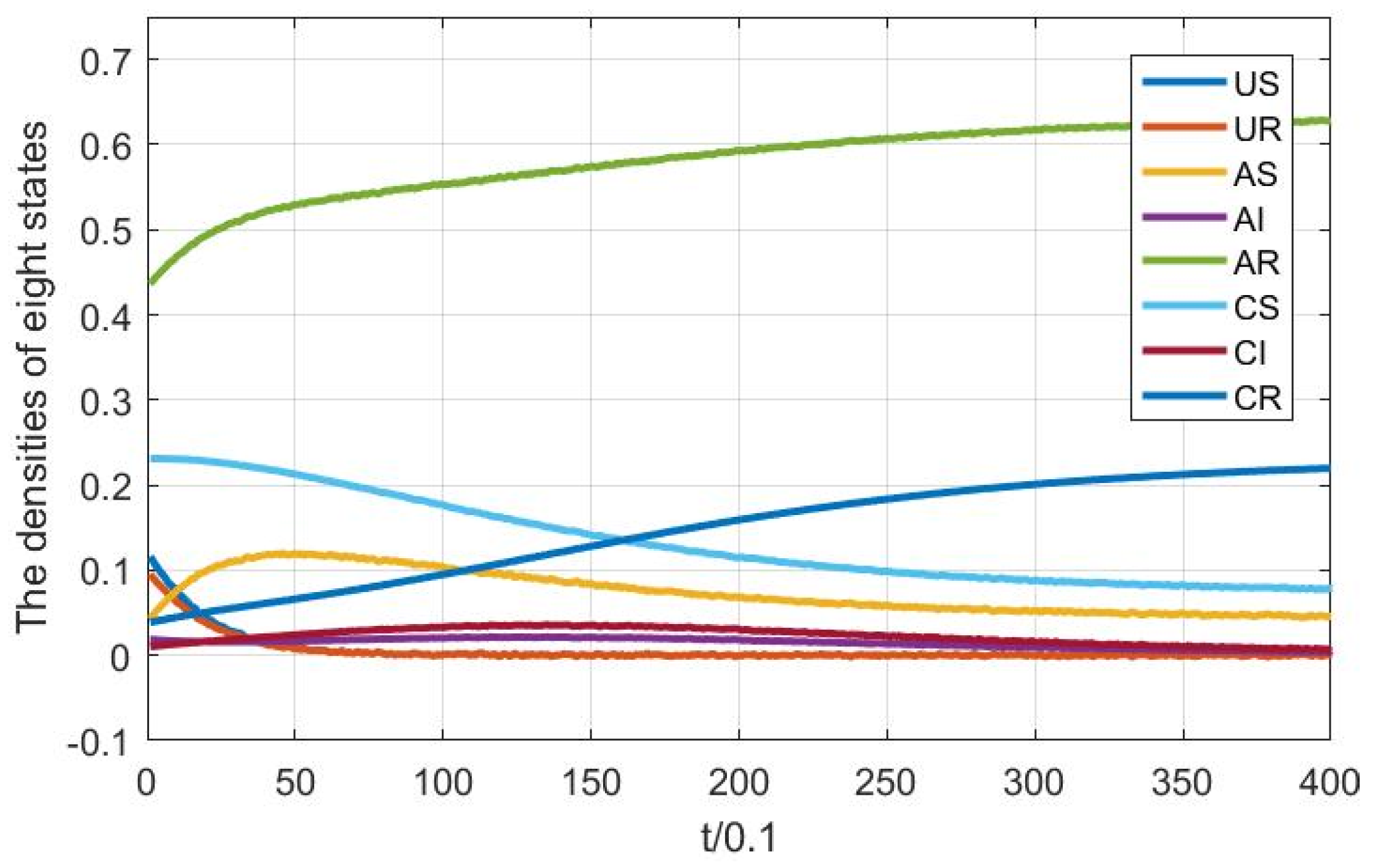
Remark 3. Compared with the results in [16,17], the simulation in Figure 6 not only presents that the infectious will disappear in the future but also shows how all the states evolve over time. We also find that all people know the information about the disease, which signifies that they will voluntarily take measures to prevent the epidemic. In addition, we also simulate the effect of the fractional order parameter on disease transmission. When we choose
, from
Figure 8, we can also find that the disease-free equilibrium point is globally asymptotically stable. However,
Figure 9 shows that the infectious states AI and CI converge much slower compared with
Figure 7. Moreover, we can conclude that the smaller the fractional order parameter, the slower the infective rate converges, as can be seen from
Figure 10.
Figure 11 indicates that under targeted immunity control, not only will the disease disappear, but everyone will know about the outbreak of the disease.
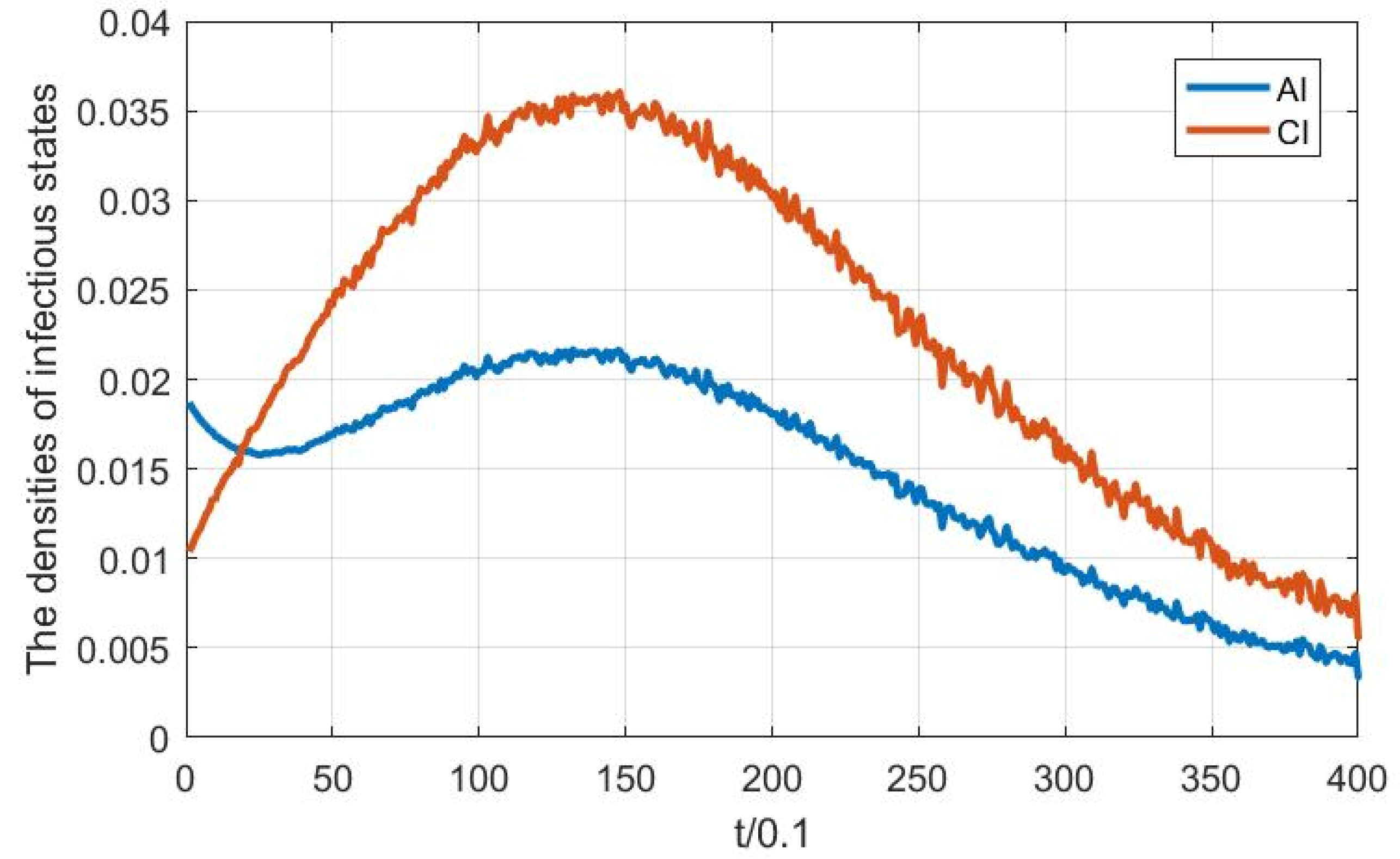
Remark 4. Comparing Figure 6 and Figure 11, it is obvious that the disease dies out much more quickly under control than no control, although it is roughly specified about the control node weight and control proportion. In the next step, we will build a real network to seek the optimal control nodes and control proportion, according to the actual situation of node weight. Example 2. For node , suppose that , , , . Other parameters are the same as Example 1, that is to say, , , weights are valued as a random number from 0 to 1, and the initial condition is also [0.122, 0.1, 0.038, 0.019, 0.432, 0.231, 0.010, 0.038]. In this case, we can calculate that and , which did not satisfy Theorem 1. From Figure 12 and Figure 13, we observe that without control, the infectious states do not decline to zero, and even have a trend of rising for a period of time. Remark 5. Comparing Figure 7 and Figure 13, it is easy to see that as the disease propagation rates and are different, then for the infectious density, one is obviously stable, the other may be unstable in a period. In a word, the disease network topology has a great influence on the epidemic transmission dynamics. Similarly, for the purpose of suppressing the spread of the disease among the elderly and young, targeted immunity control with
,
is still taken. At this moment, the simulation result is shown in
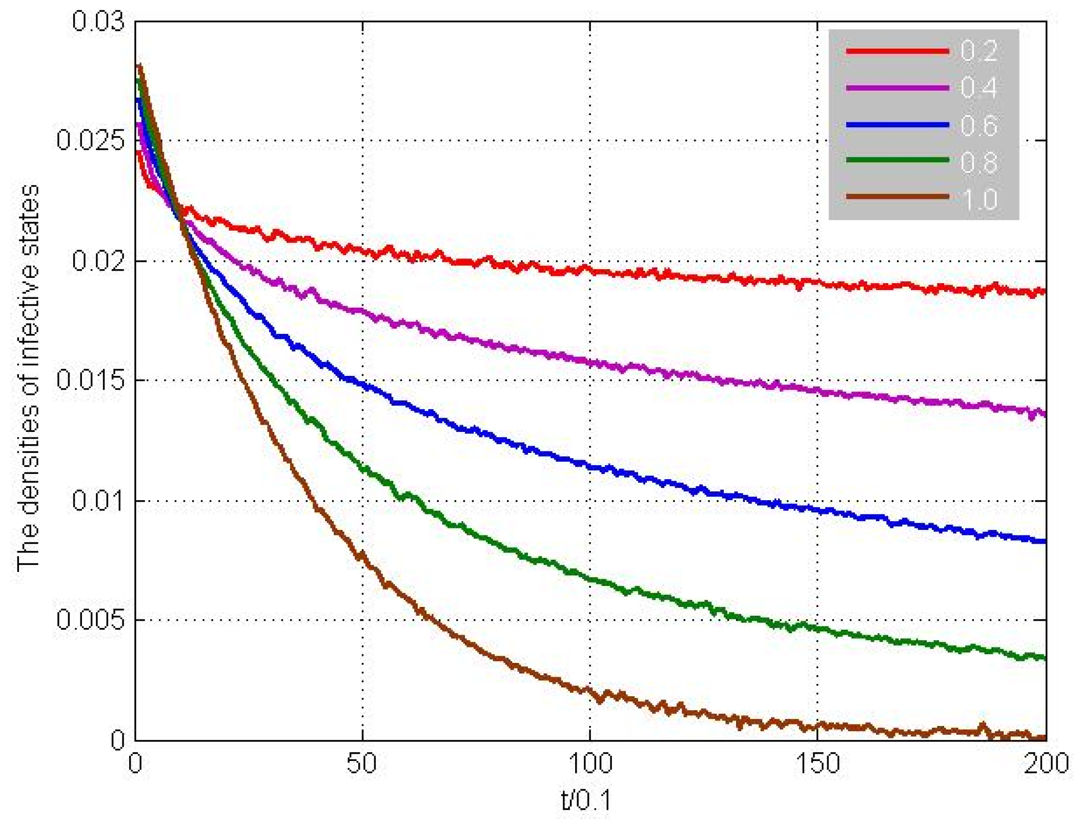
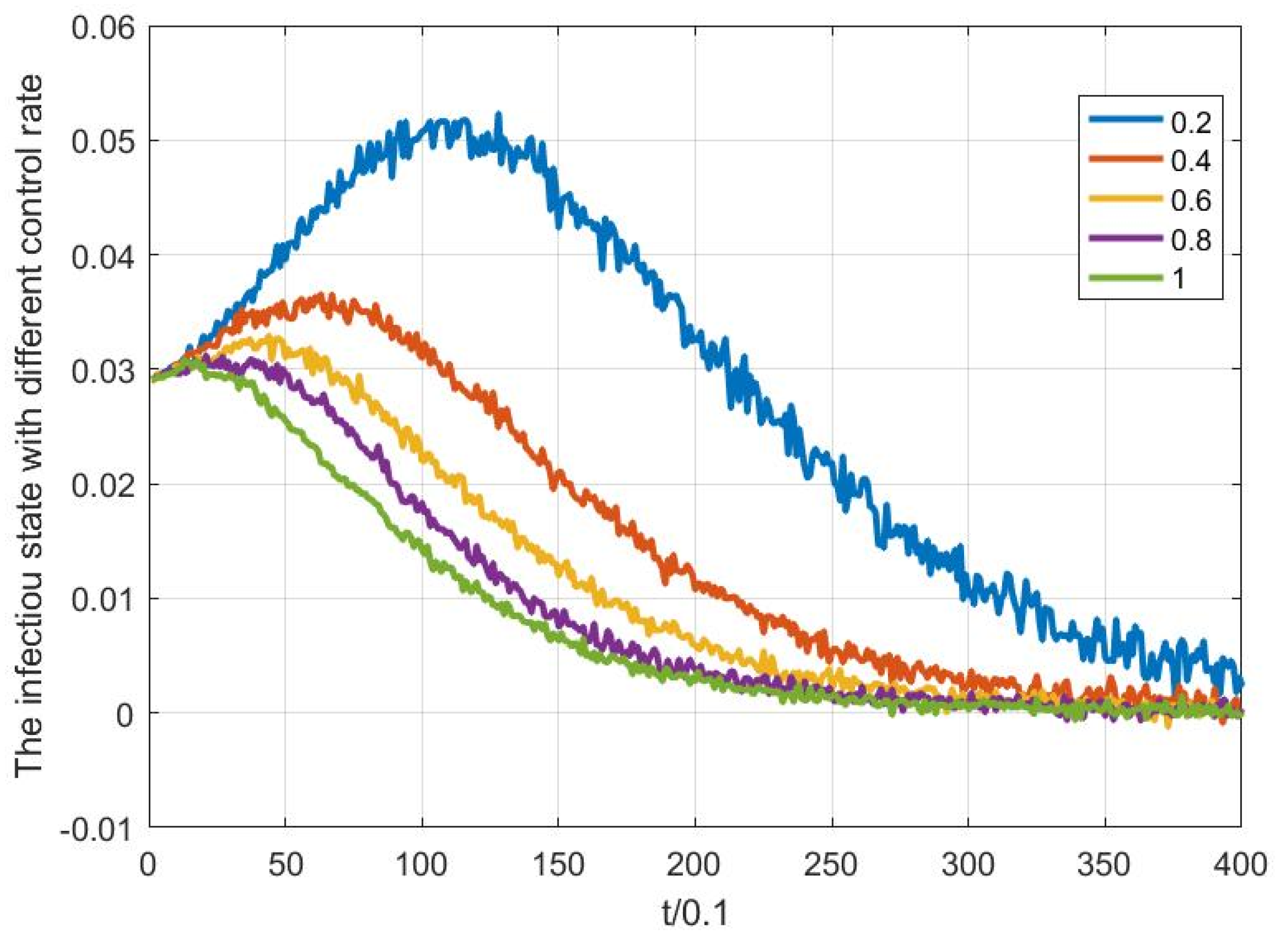
Figure 14, which indicates that the disease will disappear ultimately and the control method is effective. Moreover, with different control rates, from
Figure 15, we can observe that the larger the control rate, the more quickly the infectious state decreases. The best control effect happens when
, but the control cost is the highest.
6. Conclusions
The connection between individuals has a significant impact on the spread of disease. In order to quantitatively investigate the effect of edge weight on the spread of an epidemic, this article presents a fractional SIR model with a two-layer weighted network. On the basis of the Jacobian matrix, the stability of disease-free equilibrium is analyzed in detail. Under certain conditions, the disease-free equilibrium is locally stable, which means that the disease will eventually die out, regardless of the initial density of the infected individuals. Furthermore, we conclude that there exists no endemic equilibrium. Since the elderly and the children have lower immunity, a targeted immunity controller based on age structure is proposed. In addition, its transmission dynamics are analyzed in detail. Finally, numerical simulations are presented to illustrate the theoretical results, and the effect of the fractional order parameter on the infection rate is simulated.
Note, that since the weight has a large influence on the propagation dynamics, it may be necessary to further build a specific model and develop control strategies for certain specific infectious diseases. Many scientific disciplines are currently investigating and forecasting the spread of COVID-19. They found that older people and young children are more susceptible to COVID-19. Susceptible people have a relatively small weight in the population network. In this case, the idea is to prioritize vaccination to the nodes with less weight to prevent widespread COVID-19 infection. This strategy has worked in Zhejiang Province, China, and after a period of observation, it will be extended to the entire country. Therefore, the next research work is to analyze the critical weight parameter and calculate the optimal inoculation ratio in a real environment, although a little work has been done in this paper.


