Modeling the Chemical Pollution of the Area by the Random-Addition Method

Abstract

Currently, a significant group of industrial facilities can be classified as chemically hazardous facilities (CHFs). To predict the spread of harmful impurities in the programs being developed, Gaussian and Lagrangian models are actively used, on the basis of which the complexes used both in the EMERCOM of Russia and in research organizations are being implemented. These complexes require the introduction of a large amount of information, including the characteristics of the wind field in the distribution of an emergency chemically hazardous substance, which limits their use. In systems, the formation of which is influenced by a large number of different random factors, spatial scaling (similarity) is often found, and one or another parameter can be described using the methods of fractal geometry, which in the past few decades has been actively and successfully applied to the description of various physical objects. The purpose of this study is to analyze the possibility of using the random-addition method for early prediction of the distribution of harmful impurities in the surface air layer during the short-term release of a substance on the surface as a result of an emergency.

1. Introduction

Pollution in any form (air, water, or land) affects almost all life on Earth so quickly that its adverse effects are becoming more noticeable every day. Many researchers pay attention to the issues of environmental pollution. At the same time, the current trends in the state of the industry, despite the serious efforts being made to ensure industrial safety, not only do not exclude the occurrence and development of accidents with significant consequences, but also suggest that the possibility of increasing the corresponding risks in the medium term should be taken seriously. The spatial distribution of chemically hazardous objects, which are often located in large agglomerations, is also important here. In addition to the immediate danger posed by these emergencies, it is necessary to take into account the significant, and in some cases irreparable damage that accidents cause to ecological systems [1].

Air pollution is now considered one of the most severe environmental health risks. Consequently, there is a great need to detect, research, and analyze various sources of air pollution and their impact on the environment [2,3,4,5].

Numerous studies have shown that chronic exposure to poor air quality puts people at increased risk of heart attacks, lung cancer, strokes, and other severe life-threatening conditions. For this reason, strong demand has been directed at the scientific community to provide reliable and accurate solutions to combat the health effects of air pollution [6,7].

The article [8] focused on analyzing data on pollution from government sources and forecasting its possible future level using artificial-intelligence tools. Modeling and forecasting the level of carbon monoxide (CO) in the atmosphere was carried out, taking into account vehicle emissions as the primary source of environmental pollution.

In [9], a modification of the classical Newton method for finding a numerical solution of the constructed mathematical models in order to identify the parameters of an environmental pollutant was developed.

The main consequences of chemical accidents can be the destruction and burning of buildings, equipment, production lines, etc., the pollution of the environment (atmospheric air, earth, subsoil, soil, water, flora and fauna, buildings, structures, technological equipment, etc.), and the defeat of people. The most characteristic feature of chemical accidents involving a release (spill) is the formation of zones of chemical contamination. The size of the chemical-contamination zone depends on the physical and chemical properties, toxicity and the number of harmful chemicals released into the atmosphere (spills), as well as the meteorological conditions under which the accident occurred.

The dimensions of the zones of chemical contamination are characterized by the depth of the spread of a cloud of contaminated air with damaging concentrations, the area of the spill of an emergency chemically hazardous substance (ECHS), and the area of the zone of chemical contamination.

The main characteristic of a chemical-contamination zone is the depth of propagation of a cloud of contaminated air. It is determined by the depth of propagation of a primary or secondary cloud of contaminated air. The depth largely depends on meteorological conditions, terrain, and the building density of objects. The vertical stability of the surface air layer has a significant effect on the depth of the chemical-contamination zone: inversion (when the lower air layers are colder than the upper layers), isotherm (the air temperature at heights up to 30 m from the Earth’s surface is almost the same), convection (the lower air layer is heated more than the upper one). Inversion promotes cloud propagation over significant distances from the accident site compared to isothermal and convection. Minor depth of propagation of hazardous chemicals is observed during convection. An increase in temperature and an increase in wind speed lead to an increase in the mixing of the lower and upper layers of the atmosphere and a decrease in the depths of propagation of damaging concentrations.

A significant influence on the depth of distribution of a cloud of contaminated air is exerted by the nature of the terrain, its relief (plain-flat, plain-wavy, plain-hilly, ravine-gully, hilly), as well as the roughness of the underlying surface (open water surfaces, grass, forests, etc.). When a cloud passes through settlements, the depth of its propagation is affected by its development, as well as the air temperature in settlements [10].

A significant influence on the depth of distribution of a cloud of contaminated air is exerted by the nature of the terrain, its relief, as well as the roughness of the underlying surface (open-water surfaces, grass, forests, etc.). When a cloud passes through settlements, the depth of its propagation is affected by its development, as well as the air temperature in the settlements. The nature of the spread of hazardous chemicals in the atmosphere also largely depends on the vapor density of the hazardous chemicals. The lower the density of the hazardous chemicals, the higher the productivity of the source of infection (evaporation rate) [11].

The direction of propagation of a cloud of air contaminated by ECHS vapors with a relative density of less than one is determined by the direction of the wind, and with a relative density greater than one, both by the direction of the wind and by the profile of the terrain. ECHSs that are heavier than air spread over low places and flow into houses’ basements, retaining their damaging properties for a long time.

An essential characteristic of chemical-contamination zones is the duration of exposure to a cloud of contaminated air by the people who find themselves in the affected area of the hazardous chemicals. It is determined by the time of evaporation of the spilled hazardous chemicals or the duration of the combustion of substances that form toxic aerosols.

The evaporation time of hazardous chemicals depends, first of all, on the amount of the spilled substance, its physical and chemical properties, the area of the spill, ambient temperature, wind speed, and several other conditions.

With an increase in temperature and wind speed in the surface layer of the atmosphere, the rate of the evaporation of hazardous chemicals from the spill surface increases, which leads to a reduction in the time of exposure of hazardous chemicals to the environment and people.

At the current stage, it is possible to use several approaches for predicting the spread of harmful impurities in the atmosphere, which are associated with accidents at chemically hazardous facilities and radioactive contamination of the area, the spread of allergens, and other similar situations.

Gaussian and Lagrangian models have been developed and are actively used, based on which software systems have been introduced, both in the EMERCOM of Russia and in research organizations. However, these complexes require the introduction of a large amount of information, including the characteristics of the wind field in the zone of distribution of an emergency chemically hazardous substance, which significantly limits their use.

In systems, the formation of which is greatly influenced by several different random factors, spatial scaling (similarity) is often found, and one or another parameter can be described using the methods of fractal geometry, which in the past few decades has been actively and successfully applied to the description of various physical objects (phenomena). From the breakdown of the dielectric, e.g., the formation of the underlying rocks’ structure, to the diffusion processes, e.g., Brownian motion. Curiously, some of the first objects to which the modeling of these methods was applied were the terrain and the shape of the clouds.

The emergence of self-similarity among various physical objects with the indicated stochastic nature of the mechanisms that define these objects justifies the consideration of the possibility of applying fractal-geometry methods to the wind field of the surface layer of air, and building on this version of the model in order to predict the transport of harmful impurities in the atmosphere, which is the novelty of this work. Among the methods that make it possible to model fractal surfaces, one of the simplest and most universal methods is the Foss method (random additions), which was initially developed for one-dimensional surfaces but was later generalized to a more significant number of dimensions and can be applied both to surfaces and volumetric variants of the simulated surface. The random-addition method (Foss) is performed in the following sequence: the height $Z=0$ is fixed in the corners of the grid and in the middle of the edges of $L\times L$ elements (stage $n=1$); interpolation is carried out in the middle of the grid using already existing points, and an independent Gaussian random number $g$ with zero mean and unit variance is added to them (stage $n=2$). At the next stage, interpolation is also carried out at four new points and an independent Gaussian random number $g$ with zero mean and reduced variance is added to them. The procedure is repeated until the required scale is reached [12].

Purpose of the article: to analyze the possibility of using the method of random additions for the early forecasting of the distribution of harmful impurities in the surface layer of air during a short-term release of a substance on the surface as a result of an emergency at a chemical facility. To achieve this goal, the following tasks were set: analysis of accidents at the CRP; consideration of applied forecasting methods; analysis of the possibility of using fractal geometry methods for modeling the distribution of hazardous chemicals; determine the similarity dimension for the wind field in the surface air layer; apply the method of random additions to simulate the spread of hazardous chemicals in various conditions for the surface air layer for a short-term release of the substance; compare the results of applying this model with the current guidance document for this type of accident.

The object of this work is the issue of reducing the risks for the population and personnel in cases of accidents at chemical facilities by reducing the uncertainty in predicting the chemical situation.

The subject of this work is the possibility of using the random-addition method for modeling the propagation of hazardous chemicals in the surface air layer.

2. Materials and Methods

Many complex natural structures can be quantitatively described within the framework of the concept of fractal dimension, which is a quantity that characterizes the geometric structure of stochastic objects. Fractal geometry allows for the description of many irregular geometric shapes found in the surrounding world. These shapes can be of various dimensions: all kinds of lines (coastline, Koch curve, etc.), surfaces (terrain), and volumetric bodies (clouds).

One-dimensional, two-dimensional, and three-dimensional fractal surfaces can be modeled by various methods, one of which is the Foss method (random additions) [13,14,15,16,17].

As Foss showed, the algorithm can be easily generalized to many dimensions, i.e., applied to a 2D or 3D surface [18].

Modern approaches to modeling the chemical environment are based on various solutions of the semi-empirical equation of turbulent diffusion. Various methods yield satisfactory results for the spread of harmful substances under relatively stable surface-air-layer conditions. In cases of accidents at a chemically hazardous facility in conditions when the uncertainty of the spatial and temporal characteristics of the wind in the surface air layer is high, other approaches to modeling the chemical pollution of the area are needed. It is difficult to take into account, in one analytical form or another, a large number of independent causes affecting a bulk source of chemical pollution. This requires a large amount of initial data for forecasting, and even if they are available, one cannot avoid the significant uncertainty in the values of individual and collective risks for the population.

The basis for the application of this method is that a self-similar surface can be formed under the action of a large number of different random factors of different scales, such as their impact. So, during the formation of the relief, a large number of random factors act on it, from the movement of lithospheric plates to the processes of surface erosion, but as a result of their combined action, a specific self-similar surface is obtained that is described by a small number of parameters. In this case, the Hurst exponent H (dimension of similarity).

The vector wind field existing in the atmosphere, especially in the surface layer, is characterized by the same self-similar structure. On a large scale and a small scale, the corresponding patterns of the wind distribution turn out to be self-similar.

According to the measurement results, the appearance of the resulting density of chemical contamination of the territory is similar to an altitude (hypsometric) map of the area, a map of atmospheric pressure values or a precipitation map (Figure 1).

The formal similarity between the characteristics of the processes that form the relief and the processes that form the distribution of harmful substances on the ground as a result of an accident under conditions of uncertainty in the behavior of the atmosphere is the basis for the use of fractal-geometry methods for predicting the chemical situation, the main factor of which is the behavior of the surface air layer.

2.1. Mathematical Model of Chemical Pollution

Of great importance for visualizing geometric objects are various images, which are currently easy to obtain using the computing power of technology. Such geometric objects can be fields of physical quantities of arbitrary nature of various dimensions, arising from the simultaneous action of a large number of arbitrary random factors. One example is the distribution of chemicals on the ground. The characteristics of this distribution are a factor on which the chemical safety of the population depends. This can only be provided when the analyzed risks yield acceptable values [18,19,20,21,22,23]. The main stages of risk analysis and forecasting are shown in Figure 2.

The lack of information on the values regarding the chemical factor actualizes the task of predicting it for the subsequent determination of the impact on the population of the polluted territory. This impact cannot be predicted without taking into account, on one hand, the stability of the natural systems themselves, and on the other, the uncertainty of the chemical effects [24].

Thus, the main problem of chemical safety, the solution of which is based, on one hand, on the analysis of the dynamics of the behavior of natural systems, and on the other, on the assessment of the uncertainty of chemical effects arising under the influence of random factors, can be qualified by predicting the individual and collective chemical risks (Figure 3).

Currently, two main methods are used for constructing zones of chemical contamination of an area: probabilistic and deterministic. However, neither one nor the other is sufficiently effective in predicting the consequences of exposure to harmful factors, since the probabilistic technique determines large areas of infection and the deterministic technique is not accurate enough [25]. In this regard, it is urgent to improve the method for constructing zones of chemical contamination of the area, making it possible to combine probabilistic and deterministic methods.

2.2. Distribution of a Harmful Substance in an Isotropic Homogeneous Case

The modeling of the chemical contamination of an area is carried out by the ratio of the density of contamination of the territory with the height of the surface, while also creating the possibility of modeling the dynamics of changes such as contamination. The initial data for considering such a model can be taken from the nature of the chemical pollution of the area, modeled by the above algorithm, which we will call the base surface. Consider the case when a harmful substance is simultaneously released in a certain spherical volume with an initial concentration of $C_0$.

In this case, due to the emerging concentration gradient, the zone in which the substance has a certain threshold concentration $C_p$ will expand, forming at each moment a sphere with a radius r. As this area expands outside of it, a zone will also arise for which the concentration is below the threshold, but after some time, when the radius of this zone is reaches the value $r_{max}$, it is replaced by its decrease because the concentration will become less than the threshold. Ultimately, the zone’s radius will be zero, i.e., the substance will dissipate in a large volume with a low concentration.

This change in the radius of the zone of dangerous concentration can be represented in the following model: a sphere with a certain radius intersects a plane moving at a given speed. The figure in the cross-section of this plane forms a concentration zone exceeding the threshold value $C_0$ (Figure 4).

In the literature [26,27,28,29] it has been repeatedly indicated that the influence on the spread of harmful substances in the atmosphere is exerted by two groups of factors associated with the movement of the medium: its large-scale movement and the chaotic, turbulent movement of particles.

If the first is reduced to the movement of the entire zone in the space as a whole, then the second leads to a complex change such as the shape of the volumetric source of pollution. However, both the first and the second are characterized by random changes that depend on many factors and do not lend themselves to a simple definition. At the same time, the complex nature of the change in this turbulent motion allows us to consider the final nature of the change in the shape of the volumetric source as a specific three-dimensional fractal surface via the analogous methods of modeling the terrain.

Let us make two simplifying assumptions:

1. Note that the case under consideration is symmetric concerning the large circle of the sphere; therefore, the first part can be considered as movement from top to bottom, and the second as movement from bottom to top. In this case, the speed of movement of the cutting plane itself will be different at these stages and is not constant over time.

2. We will consider the change in the shape of the boundary of an external source in the frame of reference of the center of mass, which makes it possible to ignore large-scale flows of the medium.

Under such assumptions, the reference surface will be a hemisphere of a certain radius $r_{max}$, and the secant surface initially moves from bottom to top and then from top to bottom (Figure 5).

The rugged nature of the mixing of hazardous substances will lead to the fact that this supporting surface will change in a complex way, and the nature of this change will be determined by a multitude of random, independent influences.

2.3. Construction of the Reference Surface

Note that a hemisphere can be represented in a two-dimensional surface as a set of level lines of a given height, representing circles of radius $r_h$, where the index $h$ means that this radius corresponds to a certain height (Figure 6).

The effect of turbulent mixing will lead to the hemisphere being curved in a complex way, then turned into a relief surface using known modeling methods.

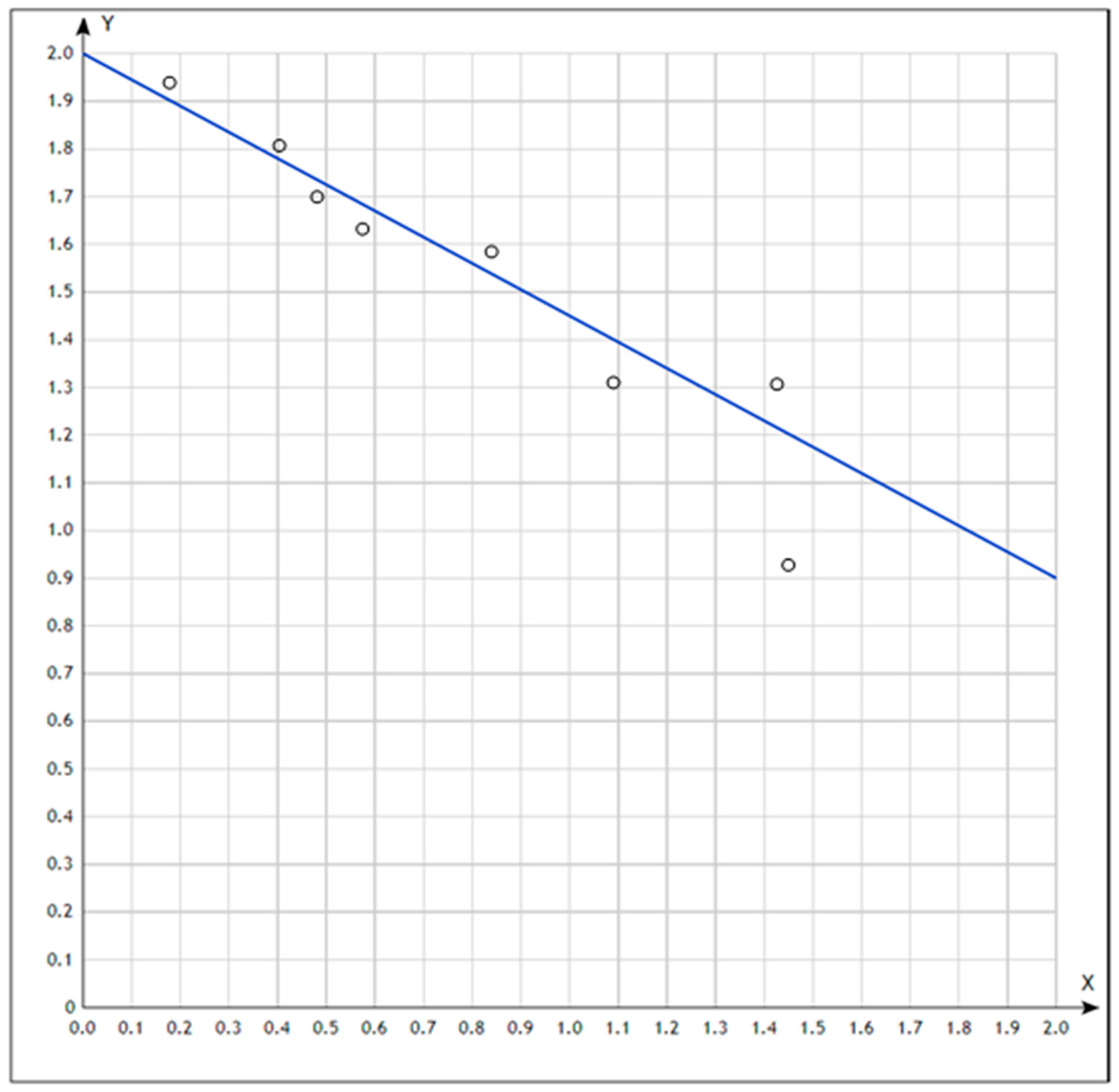
The Hurst coefficient of this surface is taken to be the same as that obtained for the distribution of projections of wind speeds on the axis. This coefficient was determined by the Korczak method, and the available data had a value of 0.9 (Figure 7) where the logarithm of the area of the corresponding sections was plotted on the ordinate, and the logarithm of the length scale was plotted on the abscissa. In the Korczak method, a section of the curve under study is marked by horizontal straight lines parallel to the abscissa axis. As a result of this procedure, a set of segmented sections is obtained, for which the cumulative distribution function $N\left(w\right)$ is constructed, which is the number of segments $N$ with a length exceeding the value of $w$. To obtain statistics sufficient for analysis, it is necessary to have about 10 sections in the range from 10% to 90% of the total range of the curve height in the studied interval. As a rule, the segments that lie both above and below the curve are included in the statistics. However, in some cases, it is interesting to study only one type of segment. The dependence $N\left(w\right)$ for a self-affine curve with fractal dimension $D$ must satisfy a simple law:

$$N\left(w\right)~w^{1-D}$$

(1)

In practice, an approximation is carried out by an expression that takes into account the effect of limiting the scaling range, which manifests itself in the method:

$$N\left(w\right)=k·w^{1-D}·\exp \left(-w/\xi \right),$$

(2)

where $k$ is the normalization coefficient and $\xi$ is the correlation length. In many cases, the definition of the parameter $\xi$ turns out to be no less interesting than the definition of the proper fractal dimension $D$.

2.4. Getting the Final Distribution

Moving along the reference surface with a cutting plane, we obtain the isohypses of this surface (Figure 8), which are current zones with a concentration exceeding the threshold $C_t$.

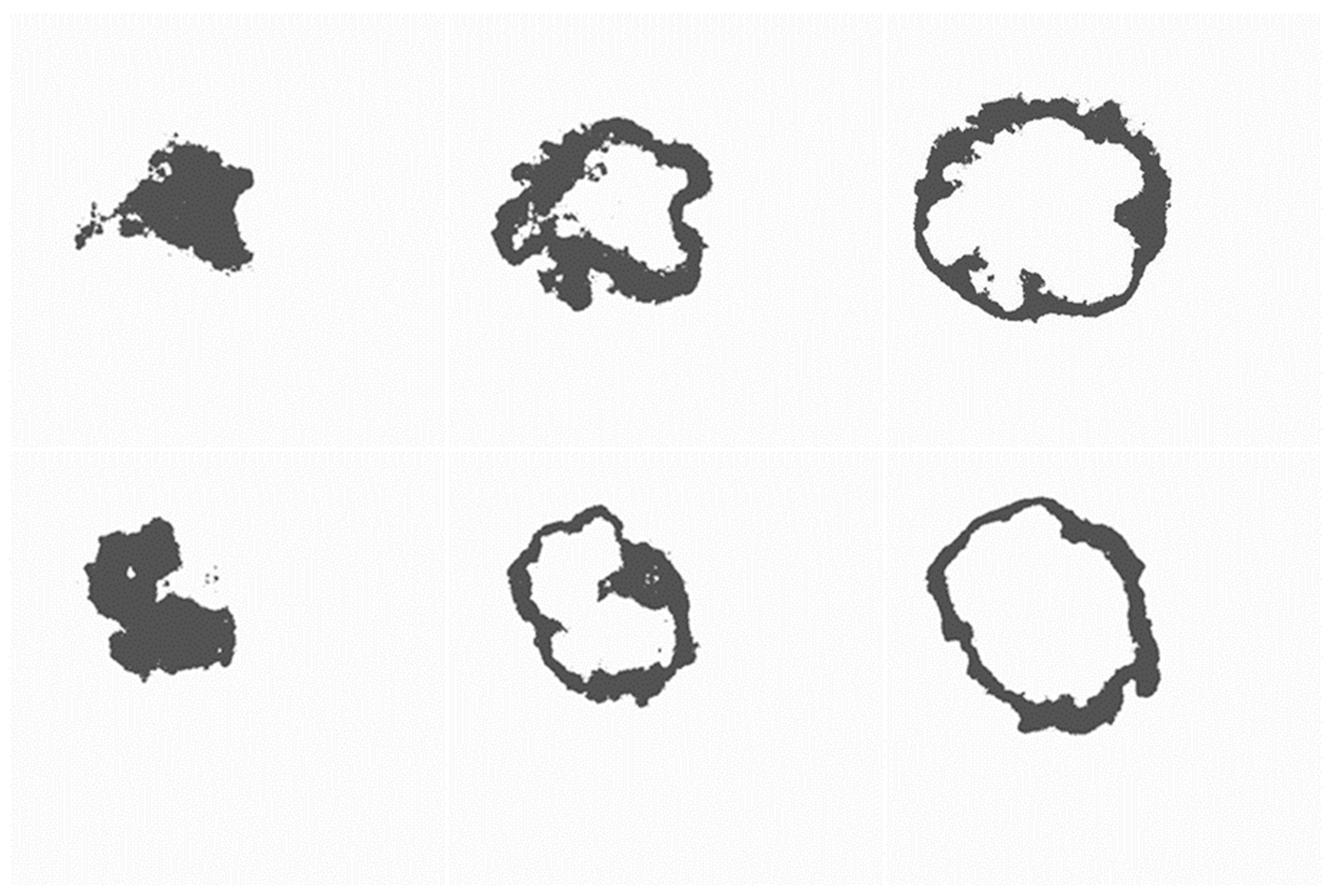
The intervals of the conditional heights of the reference surface for three different ranges of the position of the secant surface over time with two variants of the random reference surface will be similar to the randomly generated surfaces that are depicted using fractal geometry in Figure 9.

We assumed that a specific concentration $C_0$ determines the small source at the initial stage. The initial dimensions of the source can be taken into account if the motion of the secant begins not from the top point of the reference surface (infinitesimal initial volumetric source) but from a certain level $h_0$, the isoline of which will give the shape of the initial cloud. Within this zone, at a particular moment, the concentration of matter is not constant, decreasing in a complex way towards the boundaries of the cloud. Note that in the first approximation, the height of our relief surface has the same properties.

We can say that the corresponding distribution of the height in the relief surface simulates some variant of the distribution of the concentration in the focus of infection at a given time. Over time (when the cutting plane moves downward), the concentration of the substance should decrease while increasing the area of the infected zone. The final inhalation dose that a person will receive while at a given point can be estimated by summing all the values of the conditional concentration (height of the relief surface) at a given moment in time. The chemical-contamination distributions are surfaces similar to those shown in Figure 10 [30,31,32,33,34,35].

When considering the nature of the change in the concentration of harmful substances about the center of mass of the volumetric source of infection, we did not consider the source’s movement as a whole under the influence of large-scale movements of the environment (wind). If it is present, it is necessary to consider the displacement of the center of mass of the volumetric source of infection, i.e., to shift the zone by a certain distance along the OX and OY axes, which are determined depending on the wind speed.

Suppose that we know the density of pollution at three arbitrary points of the base surface $A_{i\left(sur\right)}\left(i=1, 2, 3\right)$, which we will take equal to 1.0, 3.0, and 4.0 rel. units. Using the random-addition algorithm, it is possible to construct a surface for some Hurst exponent H with a zero value of the pollution density at the four vertices of the square, which will yield in points $A_i$ some density values $A_{i\left(1\right)}$. These values will differ from the specified values $A_{i \left(sur\right)}$. The standard-deviation value measures how well the resulting surface at a given step (iteration) matches the specified values of the pollution density at points A_i of the base surface.

$${\sigma }_1={\left(\frac{1}{n}{\displaystyle \sum }_{i=1}^n{(A_{i\left(1\right)}-A_{i\left(sur\right)})}^2\right)}^{1/2}$$

(3)

The repeated execution of the algorithm in the next step will yield a new surface added to the previous one. As a result of this addition, new density values are obtained at the points $A_{i\left(2\right)}$, for which ${\sigma }_2$ is calculated provided that ${\sigma }_2<{\sigma }_1$, and a new third surface is calculated and added to the previous one. Otherwise, the calculation is performed again for the second surface. The algorithm’s execution stops when the deviation of the pollution density from the given values of the base surface becomes less than a specific small value.

Due to the random nature of the construction, the appearance of each implementation of the algorithm will differ from the base surface (Figure 11). We will evaluate the discrepancy between the base surface and the constructed one by the standard deviation σ of the pollution-density values according to the formula:

$$\sigma =\sqrt{\frac{{\displaystyle \sum }{\left(P_{0i}-P_i\right)}^2}{N}},$$

(4)

where $P_{0i}$ and $P_i$ are the values of the contamination density at the i-th point, respectively, of the base and working surfaces.

3. Results

For a qualitative and quantitative analysis of the obtained data, an example was calculated based on the current methodology for predicting the scale of contamination with potent substances in accidents (destruction) at chemically hazardous facilities and transports (RD 52.04.253-90). The following parameters were taken as the initial data: an accident involving the release of liquid chlorine from a tank located on the territory of the emergency situation of the first type (formation of only the primary cloud). The amount of leaked liquid $Q_0=5 \mathrm{tons}$, free spill. The weather was daytime, partly cloudy, +20 °C. The wind speed was <0.5 m/s. The degree of vertical stability of the atmosphere was isothermal.

Solution:

An equivalent amount of matter in the primary cloud:

$$Q=K_1{K}_3{K}_5{K}_7{Q}_0=0.18·1·0.23·1·5=0.207 \mathrm{tons},$$

(5)

where $K_1=0.18$—coefficient depending on storage conditions potent poisonous substances (PPS); $K_3=1.0$—coefficient equal to the ratio of the threshold toxic dose of chlorine to the threshold toxic dose of another PPS;$K_5=0.23$—coefficient taking into account the degree of vertical stability of the atmosphere; $K_7$—coefficient taking into account the effect of air temperature; $Q_0=5 \mathrm{tons}$—the amount of the substance emitted (spilled) during the accident.

Depth of the infected zone:

$$G=G_{min}+\left(\frac{G_{max}-G_{min}}{Q_{max}-Q_{min}}\right)·\left(Q-Q_{min}\right)=0.68+\left(\frac{1.53-0.68}{0.5-0.1}\right)·\left(0.207-0.1\right)=0.91 \mathrm{km},$$

(6)

where $G_{min}$, $G_{max}$ are the minimum and maximum values of the depth of the zone of possible infection (const); $Q_{min}, Q_{max}$ are the minimum and maximum equivalent amounts of matter in the primary cloud (const).

The area of the zone of possible infection:

$$S=8.72·{10}^{-3}·G^2\phi =8.72·{10}^{-3}·{0.91}^2·360=2.59{ \mathrm{km}}^2,$$

(7)

where $\phi =360$ at wind speed < 0.5 m/s.

Similarly, all cases were considered for an equivalent amount of a potentially toxic substance (PPS) from 0.01 to 100 tons and a wind speed from 1 to 5 m/s, approximating dependencies were derived, and correction factors were presented. The results are presented in

Table 1. Calculated results for PPS and wind speed.

Wind Speed, U, m/s	Equivalent Number of PPS, Q, g
	0.01		0.05		0.1		0.5		1		3		5		10		20		30		50		70		100
	G	S	G	S	G	S	G	S	G	S	G	S	G	S	G	S	G	S	G	S	G	S	G	S	G	S
1	0.38	0.227	0.85	1.134	1.25	2.453	3.16	15.673	4.75	35.414	9.18	132.274	12.53	246.429	19.2	578.617	29.56	1371.506	38.13	2282.037	52.67	4354.273	65.23	6678.574	81.91	10,530.836
2	0.26	0.053	0.59	0.273	0.84	0.554	1.92	2.893	2.84	6.330	5.35	22.463	7.2	40.684	10.83	92.048	16.44	212.111	21.02	346.756	28.73	647.784	35.35	980.704	44.09	1525.595
3	0.22	0.019	0.48	0.090	0.68	0.181	1.53	0.919	2.17	1.848	3.99	6.247	5.34	11.190	7.96	24.863	11.94	55.942	15.18	90.422	20.59	166.357	25.21	249.388	31.3	384.430
4	0.19	0.014	0.42	0.069	0.59	0.137	1.33	0.694	1.88	1.387	3.28	4.222	4.36	7.459	6.46	16.375	9.62	36.314	12.18	58.213	16.43	105.926	20.05	157.746	24.8	241.342
5	0.17	0.011	0.38	0.057	0.53	0.110	1.19	0.556	1.68	1.108	2.91	3.323	3.75	5.518	5.53	12.000	8.19	26.321	10.33	41.873	13.88	75.598	16.89	111.941	20.82	170.095

and Figure 12. In Figure 12, the power regression is derived, and the correlation coefficient is found.

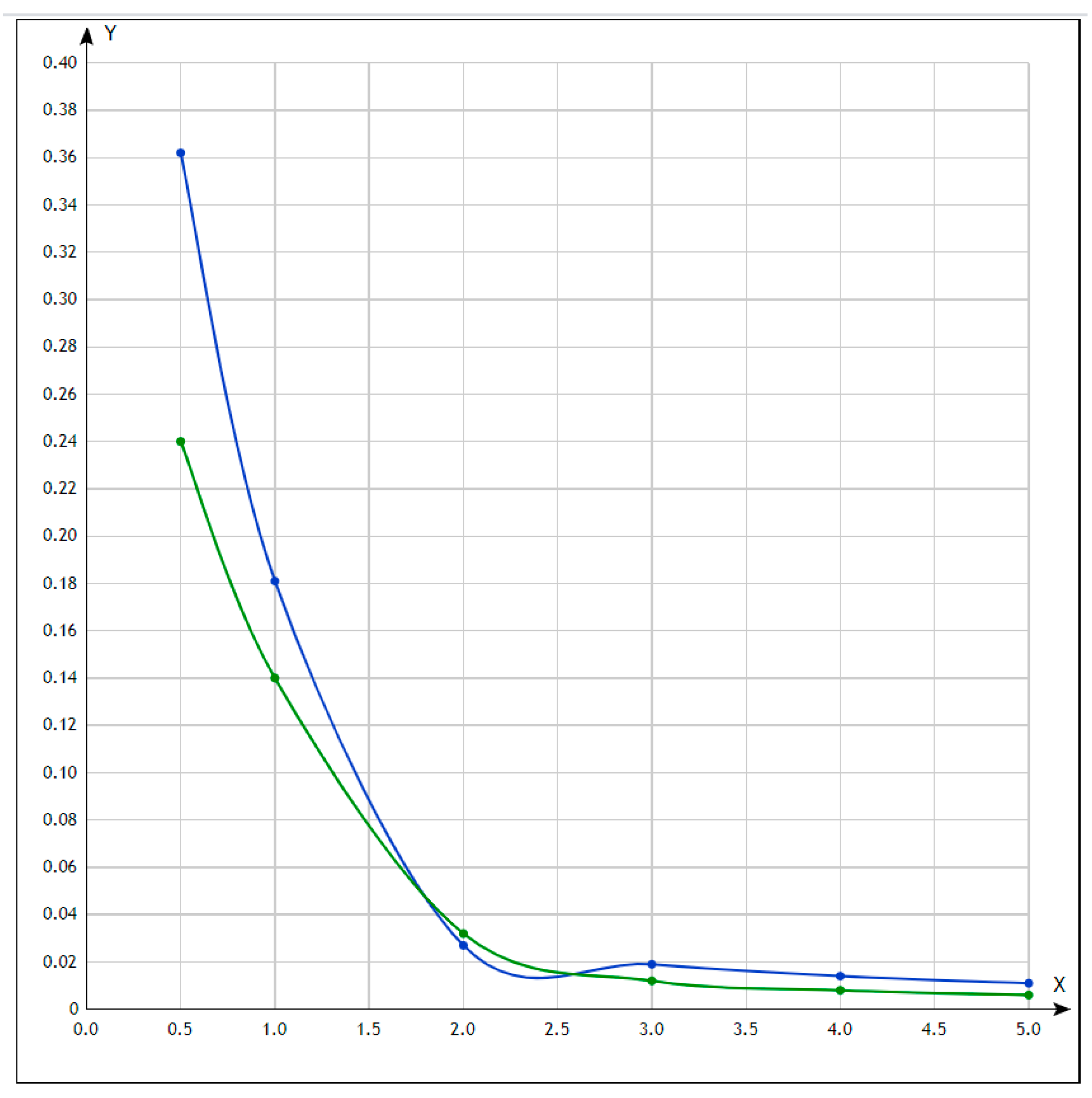
The analysis of the results allows us to conclude that the average values of the depths of infection within the selected initial data satisfactorily correspond to the existing technique, i.e., the determination of the equivalent amount of a substance from the primary and secondary cloud (RD 52.04.253-90) with some decrease for masses of more than 50 tons, thereby modeling chemical pollution. A comparison of the areas of contamination at the corresponding depths is shown in Figure 13.

The proposed model makes it possible to replace the consideration of many random factors that cause a change in the concentration of harmful substances when propagating in the atmosphere, taking into account a small number of parameters characterizing the fractal surface. The surfaces constructed with its use qualitatively correspond to the observed patterns of the distribution of impurities in the air, and can be used for volumetric sources on the analyzed scale of equivalent masses (from 0.01 to 100 tons) [36,37,38,39,40,41,42].

4. Conclusions

The relevance of this work is confirmed by the need to develop and constantly improve measures to reduce artificial risks during the operation of production facilities that store, process, or transport hazardous chemicals. The risk of such accidents is predetermined both by the complication of the operating conditions of these facilities and by other factors, including the work of personnel. An integral part of the measures is the sound and operational forecasting of the chemical situation. Based on the work performed, the following conclusions can be drawn:

The existing methods for predicting the consequences of accidents at chemical facilities, which are implemented in software systems based on semi-empirical methods, allow for the solving of a significant number of problems associated with predicting the consequences, but they presuppose the presence of a large amount of initial information related, among other things, to the behavior of the atmosphere in the surface air layer, which limits their application and simplifies the existing picture of the distribution of hazardous chemicals in the surface air layer. The distribution of wind speeds in the surface layer on a scale determined by the available data can be described by a fractal surface, which makes it possible to apply the method of random additions.

The application of this method in the range of equivalent masses from 0.01 to 100 tons at relatively low wind speeds (up to 5 m/s) shows the excellent correspondence of the approximating dependences of average depths and a decrease in the estimates of the area of probable chemical pollution in comparison with the current method (up to 25%).

An increase in the accuracy of forecasting the consequences of this type of accident helps to reduce the technogenic risk for the population and personnel of CHF.