Impact of Al₂O₃ in Electrically Conducting Mineral Oil-Based Maxwell Nanofluid: Application to the Petroleum Industry

Abstract

Alumina nanoparticles (Al₂O₃) are one of the essential metal oxides and have a wide range of applications and unique physio-chemical features. Most notably, alumina has been shown to have thermal properties such as high thermal conductivity and a convective heat transfer coefficient. Therefore, this study is conducted to integrate the adsorption of Al₂O₃ in mineral oil-based Maxwell fluid. The ambitious goal of this study is to intensify the mechanical and thermal properties of a Maxwell fluid under heat flux boundary conditions. The novelty of the research is increased by introducing fractional derivatives to the Maxwell model. There are various distinct types of fractional derivative definitions, with the Caputo fractional derivative being one of the most predominantly applied. Therefore, the fractoinal-order derivatives are evaluated using the fractional Caputo derivative, and the integer-order derivatives are evaluated using the Crank–Nicolson method. The obtained results are graphically displayed to demonstrate how all governing parameters, such as nanoparticle volume fraction, relaxation time, fractional derivative, magnetic field, thermal radiation, and viscous dissipation, have a significant impact on fluid flow and temperature distribution.

1. Introduction

Nanotechnology has been a well-known subject of study since the last century. There have been numerous groundbreaking developments in the field of nanotechnology since Nobel laureate Richard P. Feynman introduced the term in their well-known 1959 lecture “There’s Plenty of Room at the Bottom” [1]. Nanotechnology can generate a wide variety of new materials and devices with applications in nanomedicine, nanoelectronics, biomaterials, energy production, and consumer products. A decade ago, nanoparticles were studied because of their size-dependent physical and chemical properties. Now they have entered a period of commercial exploration [2]. In 1993, when industries and science needed better thermal capacities in fluids used daily for multiple jobs, Masuda et al. [3] proposed using ultra-fine particles in ordinary fluids. Later, Choi and Eastman [4] introduced the groundbreaking concept of nanofluid, which involves incorporating metallic nanoparticles with an average size of 100 nm into traditional fluids to improve thermal conductivity; this concept has modernized the worlds of engineering and industry. A nanofluid is an effective and practical approach to enhance heat transfer in a thermal system. However, research has shown that heat transfer efficiency varies between nanoparticles. Islam et al. [5] discussed the natural convection flow and heat transfer of Cu–water nanofluid into a square enclosure with the dominance of periodic magnetic effects. They observed that the heat transfer rate rises by 18.71% for Cu–water nanofluid with 1% nanoparticle volume. Wakif et al. [6] numerically investigated Couette flow with heat transfer for a Cu–water nanofluid in the presence of a magnetic field and thermal radiation with variable thermo-physical properties. Their results showed that heat transfer rates could enhance by increasing the nanoparticle volume fraction and the value of the radiation parameter. Xia et al. [7] discussed the dynamics of an unsteady reactive flow of a viscous nanomaterial subjected to Ohmic heating, heat source, and viscous dissipation. Their findings indicate that the temperature increases for the Eckert number, whereas the magnetic parameter shows the opposite pattern. Precisely, nanoparticle type, shape, and size have proven to play an important role [8,9,10].

Alumina (Al₂O₃), often known as aluminum oxide, is an amphoteric oxide found in nature in the minerals corundum and gibbsite. Alumina nanoparticles offer several desirable qualities, including high thermal conductivity, thermal stability, oxidation, high strength and stiffness, mechanical strength, high adsorption capacity, and electrical insulation. Most importantly, it is a low-cost, non-toxic, and pretty abrasive nanoparticle [11]. Haridas et al. [12] have experimentally evaluated the performance of Al₂O₃ and SiO₂ in de-ionized water-based nanofluids for their ability to influence heat transfer phenomena in small channels. They found an increase of ≈41% in the average heat transfer coefficient for the 0.02 Vol.% of Al₂O₃ at Re = 342, In contrast, the corresponding enhancement for SiO₂ nanoparticles was limited to 6% in the lower Reynolds number range. Animasaun [13] used a modified version of the buoyancy-induced model to study the flow of 47 nm alumina–water nanofluid along a horizontal paraboloid of revolution under the effects of Lorentz force, non-linear radiation, and chemical reaction. He concluded that the heat capacity and other features of 47 nm alumina–water nanofluid considerably create more heat energy at large values of volume fraction, which accounts for the overshoot in temperature and velocity curves. Kabeel and Abdelgaied [14] have numerically explored the impact of Al₂O₃–water concentration on sharp-edge orifice flow characteristics in cavitation and non-cavitation turbulent flow regimes. According to their findings, when the nanofluid concentration increases from 0.0% to 2%, the turbulent kinetic energy and turbulent intensity increase by 160% and 74%, respectively, in the separation zone downstream of the orifice. Hawwash et al. [15] looked into the effectiveness of employing alumina nanofluids as a working fluid for solar water heaters. Sheikholeslami and Ebrahimpour [16] used Al₂O₃/water together with multi-way twisted tape for thermal improvement of a linear Fresnel solar system. Bahari et al. [17] presented research on the synthesis of Al₂O₃ to SiO₂/water hybrid nanofluid and effects of anionic (SDS), cationic (CTAB), and nonionic (PVP) surfactants toward dispersion and stability. They concluded that SDS could positively affect the dispersion and stability of the nanofluids, and the best ratio of Al₂O₃:SiO₂ was at 30:70. Moreover, the electrical conductivity increased with temperature, and nanofluid containing CTAB and SDS had a higher increment in conductivity. Recently, Ho et al. [18] investigated the cooling efficiency and entropy generation of Al₂O₃–water flow and heat transfer in a circular tube with wall conduction effects. They stated that the irreversibility of a system could reduce using nanofluid.

In the late nineteenth and early twentieth centuries, it had recognized that the stress in a fluid could have a nonlinear or temporal dependency on the rate of deformation or both; we now refer to such materials as non-Newtonian fluids [19]. Non–Newtonian fluids are usually considered more suitable and sufficient in industrial processes due to their diverse range of uses, including exotic lubricants, polymer fluid extrusion, colloidal and suspension solutions, slurry fuels, and more. Unlike Newtonian fluids, it is not easy to imagine a single mathematical model that encompasses all of the properties of non-Newtonian fluids. Therefore, several mathematical models for non-Newtonian fluids have been proposed. The Maxwell fluid model, which can predict stress relaxation, has received much attention among these models. In 1867, James Clerk Maxwell proposed the concept of Maxwell fluid, and a few years later, James G. Oldroyd popularized the idea [20,21]. Researchers have drawn to the Maxwell fluid model because of its simplicity. Megahed [22] has theoretically analyzed the steady flow of Maxwell fluid along a permeable stretching sheet subject to convective boundary conditions. The consequences of the inclined magnetohydrodynamic flow of a Maxwell fluid through a penetrable stretched plate had discussed by Shafiq and Khalique [23]. Specifically, the heat generation and absorption effects are investigated in the heat transfer phenomenon using Lie group methods.

Fractional calculus is not a new concept; its history is nearly identical to classical calculus. However, it has become more popular in the constitutive modeling of non-Newtonian fluids over the last two decades. The fundamental reason for this development is that a fractional model could express the complex properties of viscoelastic material simply and elegantly. For example, many materials have an algebraic decay during the relaxation process, which cannot be adequately characterized by the exponential relaxation moduli of conventional ordinary models [24]. However, experiments indicate that fractional models can accurately capture and link these behaviors [25,26]. According to Heymans [27], complex module expressions can result in fractional derivative constitutive models that can numerically integrate the overall loading history. Liu et al. [28] introduced a unique constitution equation comprising relaxation time parameters and distributed-order fractional operators to analyze flow and heat transfer of an incompressible Maxwell fluid over a moving plate. Yang et al. [29] explored heat transfer characteristics of a double-fraction Maxwell fluid flow subject to slip boundary conditions. Their findings showed that the fractional Maxwell fluid has a higher viscosity against fractional parameters and that the oscillation phenomenon would gradually decrease as slip parameters grow. Razzaq et al. [30] addressed the heat transfer of fractional Maxwell fluid in a circular cylinder using Laplace and Hankel transformations. Hanif [31] studied two-dimensional boundary layer flow and heat transfer of fractional Maxwell fluid with constant heating. Asjad et al. [32] investigated the effects of clay nanoparticles on an unsteady natural convection flow of Maxwell nanofluids over an infinite vertical surface. They found that oil-based nanofluid had minimal velocity compared to water-based nanofluid. Saqib et al. [33] discussed the heat-transfer properties of a Maxwell fluid in the presence of a magnetic field using the fractional Cattaneo–Friedrich Model. Bayones et al. [34] studied the peristaltic flow of fractional Maxwell fluid in a circular cylinder tube in the presence of a magnetic filed.

In this research, the physical model is based on fractional Maxwell fluid flow with accompanying heat transport over a horizontal plate with significant physical assumptions. This research is motivated by improved cooling processes caused by the interaction of Al₂O₃ nanoparticles in mineral oil. The applied magnetic field and viscous dissipation contribute to the novelty of the fractional fluid model. Moreover, there are a few instances where exact analytic solutions to the Navier–Stokes equations can be found. Therefore, the inspiring goal of this research is to introduce the Crank–Nicolson-based L1 algorithm to solve the fractional Maxwell fluid flow model. There are various distinct types of fractional derivative definitions, with the Riemann–Liouville fractional derivative and the Caputo fractional derivative being two of the most prominent in applications. Therefore, the Caputo fractional derivative has been used to integrate the fractional-order derivatives, whereas integer-order derivatives are evaluated using the Crank–Nicolson finite difference method.

2. Mathematical Formulation

This section is devoted to the detailed mathematical modeling of the fractional Maxwell nanofluid. In this regard, the following definitions will be helpful.

Definition 1.

Let $\Gamma (·)$ denote the Gamma function defined by the integral (see for instance Podlubny [35])

$$\Gamma \left(\eta \right)={\int }_{\mathbb{R}}{e}^{-\psi }{\psi }^{\eta -1}d\psi ,\forall \eta \in \mathbb{C}suchthat\mathfrak{R}\left(\eta \right)>0.$$

(1)

Definition 2.

Let $n\in \mathbb{N}$ and $\alpha \in \mathbb{C}$ with $\mathfrak{R}\left(\alpha \right)>0$ such that $n-1<\alpha <n$. Then for a function f in ${\mathcal{C}}^n\left(\mathbb{R}\right)$, the Caputo fractional derivative of order α is given by:

$${\displaystyle \frac{{\partial }^{\alpha }f\left(t\right)}{\partial t^{\alpha }}}={\partial }_t^{\alpha }f\left(t\right):={\displaystyle \frac{1}{\Gamma (n-\alpha )}}{\int }_0^t{(t-\tau )}^{n-\alpha -1}{\displaystyle \frac{{\partial }^n}{\partial t^n}}f\left(\tau \right)d\tau ,$$

(2)

where $\Gamma (·)$ is the gamma function; refer to the book [35] for detailed analysis of fractional derivatives.

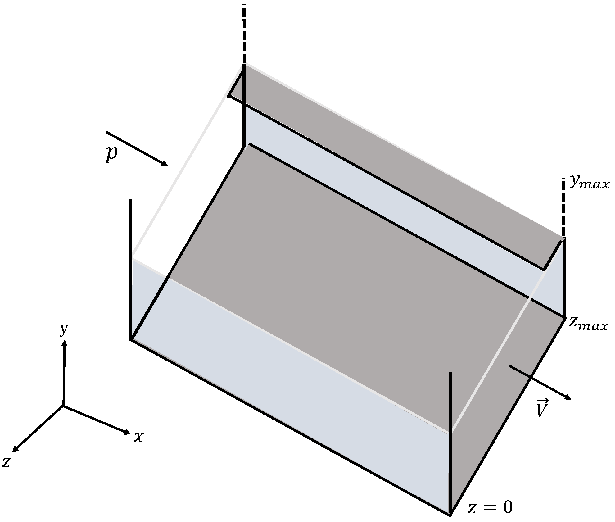
2.1. Flow Configuration and Governing Equations

Assume that the Maxwell nanofluid is in the space above an infinite plate parallel to the $xz$-plane and is confined by two parallel sidewalls perpendicular to the plate. A pressure gradient is applied to the fluid along the x-axis at time $t>0$, which initiates the mainstream flow. As a result, flow velocity takes the following form

$$V=\left(u(y,z,t),0,0\right),$$

(3)

along with the extra stress tensor

$$\mathcal{T}=\mathcal{T}(y,z,t),$$

(4)

in the absence of a cross flow. The graphical representation of the flow model is presented in Figure 1.

If a fluid with the density $\rho$ is moving with the velocity V, then the continuity equation is defined as [31]

$${\displaystyle \frac{\partial \rho }{\partial t}}+\nabla ·\left(\rho V\right)=0.$$

(5)

For an incompressible fluid, Equation (5) reduces to the following form

$$\nabla ·V=0.$$

(6)

It is simple to verify that the velocity field of the form (3) automatically meets the incompressibility condition. The non-relativistic momentum transport in any continuum is predicted by Cauchy momentum equation, defined by [36]:

$$\rho \left({\displaystyle \frac{\partial V}{\partial t}}+V·\nabla V\right)=-\nabla \mathcal{P}+\nabla ·\mathcal{T},$$

(7)

where $\mathcal{P}$ is the pressure. The extra stress tensor $\mathcal{T}$ is represented by the following relationship [34]:

$$\mathcal{T}+{\lambda }^{\alpha }\left({\partial }_t^{\alpha }\mathcal{T}+V·\nabla \mathcal{T}-\left(\nabla V\right)\mathcal{T}-\mathcal{T}{\left(\nabla V\right)}^{†}\right)=\mu \mathcal{A}.$$

(8)

Here $\mathcal{A}=\nabla V+{\left(\nabla V\right)}^{†}$ is the first Rivlin–Erickson tensor, $\mu$ is the dynamic viscosity of Maxwell fluid, $\lambda$ is the relaxation time parameter, and the subscript † is the transpose of a matrix. In the presence of magnetic field $B=B_0+B_1$, Equation (7) can be modified as

$$\rho \left({\displaystyle \frac{\partial V}{\partial t}}+V·\nabla V\right)=-\nabla \mathcal{P}+\nabla ·\mathcal{T}+J\times B.$$

(9)

Ohm’s law describes the current density J as [37]

$$J=\sigma E_r,$$

(10)

where $\sigma$ is the electrical conductivity of the fluid and $E_r$ is the electric field experienced by the fluid. Applying the Lorentz transformation to the fluid traveling at velocity V concerning the external magnetic field gives us

$$E_r=E+V\times B.$$

(11)

The electric field vector $E=0$ because no applied or polarization voltage is imposed on the flow field. Further, the magnetic Reynolds number is considered to be too small for the induced magnetic field $B_1$ to be negligible, and therefore the current density J is reduced to

$$J=\sigma \left(V\times B\right),$$

(12)

and the cross product $\left(V\times B\right)$ can be obtained as

$$\left(V\times B\right)=\left|\begin{array}{ccc}i& j& k\\ u& 0& 0\\ 0& B_0& 0\end{array}\right|=\left(0,0,B_{0}u\right).$$

(13)

With Equations (12) and (13), $\left(J\times B\right)$ is given as

$$\left(J\times B\right)=\left|\begin{array}{ccc}i& j& k\\ 0& 0& B_{0}u\\ 0& B_0& 0\end{array}\right|=\left(-B_0^{2}u,0,0\right).$$

(14)

In reference with the velocity field (3), extra stress tensor (4) and Lorentz force (14), the momentum Equation (9) reduces to the following form

$${\rho }_{nf}{\displaystyle \frac{\partial u}{\partial t}}=-{\displaystyle \frac{\partial \mathcal{P}}{\partial x}}+{\displaystyle \frac{\partial {\tau }_{xy}}{\partial y}}+{\displaystyle \frac{\partial {\tau }_{xz}}{\partial z}}-B_0^{2}u,$$

(15)

where ${\tau }_{xy}$ and ${\tau }_{xz}$ are nonzero components of $\mathcal{T}$. Introducing Equation (3) into the extra stress tensor relation (8) gives us

$$\left(1+{\lambda }_1^{\alpha }{\partial }_t^{\alpha }\right){\tau }_{xy}=\mu {\displaystyle \frac{\partial u}{\partial y}},\left(1+{\lambda }_1^{\alpha }{\partial }_t^{\alpha }\right){\tau }_{xz}=\mu {\displaystyle \frac{\partial u}{\partial z}}.$$

(16)

Now, operating the differential operator $\left(1+{\lambda }_1^{\alpha }{\partial }_t^{\alpha }\right)$ to Equation (15) and utilizing Equation (16) results in

$$\rho \left(1+{\lambda }_1^{\alpha }{\partial }_t^{\alpha }\right){\displaystyle \frac{\partial u}{\partial t}}=-\left(1+{\lambda }_1^{\alpha }{\partial }_t^{\alpha }\right){\displaystyle \frac{\partial \mathcal{P}}{\partial x}}+\mu \left({\displaystyle \frac{{\partial }^{2}u}{\partial y^2}}+{\displaystyle \frac{{\partial }^{2}u}{\partial z^2}}\right)-B_0^2\sigma \left(1+{\lambda }_1^{\alpha }{\partial }_t^{\alpha }\right)u.$$

(17)

The applied pressure in the x-direction is

$${\displaystyle \frac{\partial \mathcal{P}}{\partial x}}=p_0\mathcal{H}\left(t\right),$$

(18)

with the Heaviside function

$$\mathcal{H}\left(t\right)=\left\{\begin{array}{c}1,t>0,\hfill \\ \\ 0,t<0.\hfill \end{array}\right.$$

(19)

Next, the internal (heat) energy balance law can be stated in terms of T as [31]

$$\rho C_p\left({\displaystyle \frac{\partial T}{\partial t}}+V·\nabla T\right)=k\nabla T+\mathcal{T}:\nabla V.$$

(20)

Here k is the thermal conductivity and $C_p$ is the specific heat at constant pressure. In the presence of thermal radiation and Ohmic heating, the energy Equation (20) can be modified as

$$\rho C_p\left({\displaystyle \frac{\partial T}{\partial t}}+V·\nabla T\right)=k\nabla T-{\displaystyle \frac{\partial q_r}{\partial y}}+{\displaystyle \frac{1}{\sigma }}J·J+\mathcal{T}:\nabla V.$$

(21)

Using the Roseland approximation, the radiative heat flux $q_r$ in Equation (21) is expressed as

$$q_r=-{\displaystyle \frac{4{\sigma }_b}{3k_b}}{\displaystyle \frac{\partial T^4}{\partial y}}.$$

(22)

Let us consider that the temperature difference $T-T_{\infty }$ within the flow domain to be small enough that $T^4$ can be reasonably expanded about $T_{\infty }$ using the Taylor series as follows:

$$T^4\approxeq T_{\infty }^4+4T_{\infty }^3(T-T_{\infty })+6T_{\infty }^2{(T-T_{\infty })}^2+\dots$$

(23)

The higher-order terms are ignored because the temperature gradient is believed to be small enough, resulting in

$$T^4\approxeq T_{\infty }^4+4T_{\infty }^3(T-T_{\infty }).$$

(24)

In Equation (22), the simplified version of $T^4$ is employed and differentiated w.r.t y, yielding

$${\displaystyle \frac{\partial q_r}{\partial y}}=-{\displaystyle \frac{16{\sigma }_b{T}_{\infty }^3}{3k_b}}{\displaystyle \frac{\partial T^2}{\partial y^2}}.$$

(25)

Invoking Equations (3), (12) and (25) for the energy Equation (21) leads us to

$$\rho C_p{\displaystyle \frac{\partial T}{\partial t}}=k\left({\displaystyle \frac{{\partial }^{2}T}{\partial y^2}}+{\displaystyle \frac{{\partial }^{2}T}{\partial z^2}}\right)+{\displaystyle \frac{{\partial }^{2}T}{\partial y^2}}+B_0^2\sigma u^2+{\tau }_{xy}{\displaystyle \frac{\partial u}{\partial y}}+{\tau }_{xz}{\displaystyle \frac{\partial u}{\partial z}}.$$

(26)

Furthermore, the governing equation for a nanofluid flow can be obtained by replacing the properties of a regular fluid with the corresponding properties of a nanofluid. Hence Equations (17) and (26) can be revised as

$${\rho }_{nf}\left(1+{\lambda }_1^{\alpha }{\partial }_t^{\alpha }\right){\displaystyle \frac{\partial u}{\partial t}}=-\left(1+{\lambda }_1^{\alpha }{\partial }_t^{\alpha }\right){\displaystyle \frac{\partial \mathcal{P}}{\partial x}}+{\mu }_{nf}\left({\displaystyle \frac{{\partial }^{2}u}{\partial y^2}}++{\displaystyle \frac{{\partial }^{2}u}{\partial z^2}}\right)-B_0^2{\sigma }_{nf}\left(1+{\lambda }_1^{\alpha }{\partial }_t^{\alpha }\right)u.$$

(27)

$${\left(\rho C_p\right)}_{nf}{\displaystyle \frac{\partial T}{\partial t}}=k_{nf}\left({\displaystyle \frac{{\partial }^{2}T}{\partial y^2}}+{\displaystyle \frac{{\partial }^{2}T}{\partial z^2}}\right)+{\displaystyle \frac{{\partial }^{2}T}{\partial y^2}}+B_0^2{\sigma }_{nf}{u}^2+{\tau }_{xy}{\displaystyle \frac{\partial u}{\partial y}}+{\tau }_{xz}{\displaystyle \frac{\partial u}{\partial z}}.$$

(28)

The mathematical expressions for nanofluid properties, ${\mu }_{nf}$, ${\rho }_{nf}$, ${\sigma }_{nf}$, ${\left(\rho C_p\right)}_{nf}$, and $k_{nf}$ are presented in

Table 1. Mathematical expression of nanofluid properties [5].

Properties	Mathematical Expressions
Viscosity	${\mu }_{nf}={\mu }_f{(1-\phi )}^{-2.5}$
Density	${\rho }_{nf}=(1-\phi ){\rho }_f+\phi {\rho }_s$
Heat capacitance	${\left(\rho C_p\right)}_{nf}=(1-\phi ){\left(\rho C_p\right)}_f+\phi {\left(\rho C_p\right)}_s$
Thermal conductivity	${\displaystyle \frac{k_{nf}}{k_f}}={\displaystyle \frac{(k_s+2k_f)+2\phi (k_s-k_f)}{(k_s+2k_f)-\phi (k_s-k_f)}}$
Electrical conductivity	${\displaystyle \frac{{\sigma }_{nf}}{{\sigma }_f}}={\displaystyle \frac{({\sigma }_s+2{\sigma }_f)+2\phi ({\sigma }_s-{\sigma }_f)}{({\sigma }_s+2{\sigma }_f)-\phi ({\sigma }_s-{\sigma }_f)}}$

, and thermo-physical properties of mineral oil and Al₂O₃ are provided in

Table 2. Thermo-physical properties of mineral oil and nanoparticles [38,39].

Materials	Mineral Oil	Al2O3
$\rho$ (kg/m3)	861	3970
k (W/mK)	0.157	40
$C_p$ (J/kgK)	1860	765
$\sigma$ (S/m)	≈0.3310−9	35 × 106
$\mu$ (Pa.s)	0.01335	–

.

Initially, the fluid is at rest. Therefore, the zero initial conditions are considered:

$$u(y,z,t)=0={\displaystyle \frac{\partial u(y,z,t)}{\partial t}},T(y,z,t),t\le 0,(y,z)\in [0,\infty )\times [0,z_{max}].$$

(29)

We impose a no-slip velocity condition along the plate and the walls so that:

$$\begin{array}{c}\hfill \left\{\begin{array}{c}u(0,z,t)=0,k_{nf}{\displaystyle \frac{\partial T(0,z,t)}{\partial y}}=-q_w,t>0,z\in [0,z_{max}],\hfill \\ u(y,0,t)=0=u(y,z_{max},t),t>0,y\in [0,\infty ),\hfill \\ T(y,0,t)=T_{\infty }=T(y,z_{max},t),t>0,y\in [0,\infty ).\hfill \end{array}\right.\end{array}$$

(30)

The natural far field conditions are:

$$u(y,z,t)\to 0,T(y,z,t)\to T_{\infty }\mathrm{as}y\to \infty .$$

(31)

2.2. Non-Dimensional Modeling

Non-dimensional representation is imperative to highlight the physics of the stated problem. Therefore, the following non-dimensional parameters are introduced:

$$\begin{array}{cccc}{y}^{*}={\displaystyle \frac{y}{z_{max}}},\hfill & z^{*}={\displaystyle \frac{z}{z_{max}}},\hfill & t^{*}={\displaystyle \frac{{\nu }_{f}t}{z_{max}^2}},\hfill & u^{*}={\displaystyle \frac{u{z}_{max}}{{\nu }_f}},\hfill \\ T^{*}={\displaystyle \frac{T-T_{\infty }}{q_w{z}_{max}/k_f}},\hfill & {\lambda }^{*}={\displaystyle \frac{\lambda {\nu }_f}{z_{max}^2}},\hfill & {\tau }_{xy}^{*}={\displaystyle \frac{z_{max}^2{\tau }_{xy}}{{\mu }_f{\nu }_f}},\hfill & {\tau }_{xz}^{*}={\displaystyle \frac{z_{max}^2{\tau }_{xz}}{{\mu }_f{\nu }_f}}.\hfill \end{array}$$

(32)

Using the set of non-dimensional parameters (32) in Equations (27)–(31), we arrived at

$${\varphi }_1\left(1+{\lambda }^{\alpha }{\displaystyle \frac{{\partial }^{\alpha }}{\partial t^{\alpha }}}\right){\displaystyle \frac{\partial u}{\partial t}}=p\left(\mathcal{H}\left(t\right)+{\lambda }^{\alpha }{\displaystyle \frac{t^{-\alpha }}{\Gamma (1-\alpha )}}\right)+{\varphi }_2\left({\displaystyle \frac{{\partial }^{2}u}{\partial y^2}}+{\displaystyle \frac{{\partial }^{2}u}{\partial z^2}}\right)-{\varphi }_{3}M\left(1+{\lambda }^{\alpha }{\displaystyle \frac{{\partial }^{\alpha }}{\partial t^{\alpha }}}\right)u,$$

(33)

$$Pr{\varphi }_4{\displaystyle \frac{\partial T}{\partial t}}=\left({\varphi }_5+Rd\right){\displaystyle \frac{{\partial }^{2}T}{\partial y^2}}+{\varphi }_5{\displaystyle \frac{{\partial }^{2}T}{\partial z^2}}+{\varphi }_{3}M{u}^2+\mathcal{E}\left\{{\tau }_{xy}{\displaystyle \frac{\partial u}{\partial y}}+{\tau }_{xz}{\displaystyle \frac{\partial u}{\partial z}}\right\},$$

(34)

subject to the initial and boundary conditions

$$\begin{array}{c}\hfill \left\{\begin{array}{c}u(y,z,t)=0={\displaystyle \frac{\partial u(y,z,t)}{\partial t}},T(y,z,t)=0,t<0,(y,z)\in [0,\infty )\times [0,z_{max}],\hfill \\ u(0,z,t)=0,{\varphi }_4{\displaystyle \frac{\partial T(0,z,t)}{\partial y}}=-1,t>0,z\in [0,z_{max}],\hfill \\ u(y,0,t)=0=u(y,z_{max},t),T(y,0,t)=0=T(y,z_{max},t),t>0,y\in [0,\infty ),\hfill \\ u(y,z,t)\to 0,T(y,z,t)\to 0\mathrm{as}y\to \infty .\hfill \end{array}\right.\end{array}$$

(35)

Provided that

$$\begin{array}{c}{\varphi }_1=(1-\phi )+\phi {\rho }_s/{\rho }_f,{\varphi }_2={\left(1-\phi \right)}^{-2.5},{\varphi }_3={\displaystyle \frac{{\sigma }_{nf}}{{\sigma }_f}},{\varphi }_4=(1-\phi )+\phi {\left(\rho C_p\right)}_s/{\left(\rho C_p\right)}_f,\hfill \\ {\varphi }_5={\displaystyle \frac{k_{nf}}{k_f}},p={\displaystyle \frac{p_0{z}_{max}^3}{{\nu }_f^2}},M={\displaystyle \frac{{\sigma }_f{B}_0^2{z}_{max}}{{\mu }_f}},Rd={\displaystyle \frac{16{\sigma }_b}{3k_b{k}_f}},\mathcal{E}={\displaystyle \frac{{\mu }_f{\nu }_f^2}{q_w{z}_{maz}^3}},Pr={\displaystyle \frac{{\mu }_f{C}_{p_f}}{k_f}}.\hfill \end{array}$$

(36)

3. Numerical Scheme

The aim of this section is to devise a scheme for approximating Equations (33)–(35) over a finite time interval.

Define $t_k=k\mathsf{\hslash },k=0,1,\cdots ,\mathfrak{n}$, $y_i=i\mathfrak{p},i=1,2,\cdots ,\mathfrak{r}$, $z_j=j\mathfrak{q},j=1,2,\cdots ,\mathfrak{s}$, where $\mathsf{\hslash }=t_{\mathfrak{f}}/n$, is the time step, $\mathfrak{p}=y_{max}/\mathfrak{r}$, and $\mathfrak{q}=z_{max}/\mathfrak{s}$ are the mesh size in $(y,z)$ direction. The integer-order derivatives are approximated using the Crank–Nicolson finite difference method as follows:

$${\displaystyle \frac{\partial u}{\partial t}}{|}_{t_k}={\displaystyle \frac{u_{i,j}^k-u_{i,j}^{k-1}}{\mathsf{\hslash }}},{\displaystyle \frac{\partial T}{\partial t}}{|}_{t_k}={\displaystyle \frac{T_{i,j}^k-T_{i,j}^{k-1}}{\mathsf{\hslash }}}.$$

(37)

$${\displaystyle \frac{{\partial }^{2}u}{\partial y^2}}{|}_{t_k}={\displaystyle \frac{u_{i-1,j}^k-2u_{i,j}^k+u_{i+1,j}^k+u_{i-1,j}^{k-1}-2u_{i,j}^{k-1}+u_{i+1,j}^{k-1}}{2{\mathfrak{p}}^2}}.$$

(38)

$${\displaystyle \frac{{\partial }^{2}u}{\partial z^2}}{|}_{t_k}={\displaystyle \frac{u_{i,j-1}^k-2u_{i,j}^k+u_{i,j+1}^k+u_{i,j-1}^{k-1}-2u_{i,j}^{k-1}+u_{i,j+1}^{k-1}}{2{\mathfrak{q}}^2}}.$$

(39)

$${\displaystyle \frac{{\partial }^{2}T}{\partial y^2}}{|}_{t_k}={\displaystyle \frac{T_{i-1,j}^k-2T_{i,j}^k+T_{i+1,j}^k+T_{i-1,j}^{k-1}-2T_{i,j}^{k-1}+T_{i+1,j}^{k-1}}{2{\mathfrak{p}}^2}}.$$

(40)

$${\displaystyle \frac{{\partial }^{2}T}{\partial z^2}}{|}_{t_k}={\displaystyle \frac{T_{i,j-1}^k-2T_{i,j}^k+T_{i,j+1}^k+T_{i,j-1}^{k-1}-2T_{i,j}^{k-1}+T_{i,j+1}^{k-1}}{2{\mathfrak{q}}^2}}.$$

(41)

The L1 algorithm of Caputo fractional derivative (2) is given as

$$\begin{array}{cc}{\displaystyle \frac{{\partial }^{\alpha }f\left(t_k\right)}{\partial t^{\alpha }}}\hfill & ={\displaystyle \frac{{\mathsf{\hslash }}^{-\alpha }}{\Gamma (2-\alpha )}}{\sum }_{\mathfrak{m}=0}^{k-1}{b}_{\mathfrak{m}}\left[f(t_{k-\mathfrak{m}}-f\left(t_{k-\mathfrak{m}-1}\right)\right],\hfill \\ \hfill & ={\displaystyle \frac{{\mathsf{\hslash }}^{-\alpha }}{\Gamma (2-\alpha )}}\left[b_{0}f\left(t_k\right)-b_{k-1}f\left(t_0\right)-{\sum }_{\mathfrak{m}=1}^{k-1}(b_{\mathfrak{m}-1}-b_{\mathfrak{m}})f\left(t_{k-\mathfrak{m}}\right)\right],\hfill \end{array}$$

(42)

where $b_{\mathfrak{m}}={(\mathfrak{m}+1)}^{1-\alpha }-{\mathfrak{m}}^{1-\alpha },\mathfrak{m}=0,1,2,\cdots ,\mathfrak{n}$. Now, the fractional derivatives in Equation (33) can be approximated using the L1 algorithm (42) as follows:

$${\displaystyle \frac{{\partial }^{\alpha }u}{\partial t^{\alpha }}}{|}_{t_k}={\displaystyle \frac{{\mathsf{\hslash }}^{-\alpha }}{\Gamma (2-\alpha )}}\left[{\displaystyle u}\left(t_k\right)-\sum _{\mathfrak{m}=1}^{k-1}{a}_{\mathfrak{m}}{\displaystyle u}\left(t_{k-\mathfrak{m}}\right)\right],$$

(43)

$${\displaystyle \frac{{\partial }^{\alpha +1}u}{\partial t^{\alpha +1}}}{|}_{t_k}={\displaystyle \frac{{\mathsf{\hslash }}^{-\alpha -1}}{\Gamma (2-\alpha )}}\left[{\displaystyle u}\left(t_k\right)-{\displaystyle u}\left(t_{k-1}\right)-\sum _{\mathfrak{m}=1}^{k-1}{a}_{\mathfrak{m}}\left({\displaystyle u}\left(t_{k-\mathfrak{m}}\right)-{\displaystyle u}\left(t_{k-\mathfrak{m}-1}\right)\right)\right],$$

(44)

where $a_{\mathfrak{m}}=(b_{\mathfrak{m}-1}-b_{\mathfrak{m}})$.

$$\begin{array}{cc}\hfill {\displaystyle \frac{{\varphi }_1}{\mathsf{\hslash }}}\left(1+{\displaystyle \frac{{\lambda }^{\alpha }{\mathsf{\hslash }}^{-\alpha }}{\Gamma (2-\alpha )}}\right)\left[u_{i,j}^k-u_{i,j}^{k-1}\right]& ={\displaystyle \frac{{\varphi }_1{p}_0}{2}}\left[\mathcal{H}\left(t_k\right)+\mathcal{H}\left(t_{k+1}\right)+{\lambda }^{\alpha }{\displaystyle \frac{t_k^{-\alpha }+t_{k+1}^{-\alpha }}{\Gamma (1-\alpha )}}\right]\hfill \\ & +{\displaystyle \frac{{\varphi }_2}{2{\mathfrak{p}}^2}}[u_{i-1,j}^k-2u_{i,j}^k+u_{i+1,j}^k+u_{i-1,j}^{k-1}\hfill \\ & -2u_{i,j}^{k-1}+u_{i+1,j}^{k-1}]+{\displaystyle \frac{{\varphi }_2}{2{\mathfrak{q}}^2}}[u_{i,j-1}^k-2u_{i,j}^k\hfill \\ & +u_{i,j+1}^k+u_{i,j-1}^{k-1}-2u_{i,j}^{k-1}+u_{i,j+1}^{k-1}]\hfill \\ & -\left({\varphi }_{3}M+{\varphi }_{3}M{\lambda }^{\alpha }{\displaystyle \frac{{\mathsf{\hslash }}^{-\alpha }}{\Gamma (2-\alpha )}}\right)\left[u_{i,j}^k+u_{i,j}^{k-1}\right]\hfill \\ & +{\varphi }_{3}M{\lambda }^{\alpha }{\displaystyle \frac{{\mathsf{\hslash }}^{-\alpha }}{\Gamma (2-\alpha )}}{\sum }_{\mathfrak{m}=1}^{k-1}{\mathfrak{b}}_{\mathfrak{m}}\left[u_{i,j}^{k-\mathfrak{m}}+u_{i,j}^{k-\mathfrak{m}-1}\right]\hfill \\ & +{\varphi }_1{\lambda }^{\alpha }{\displaystyle \frac{{\mathsf{\hslash }}^{-(\alpha +1)}}{\Gamma (2-\alpha )}}{\sum }_{\mathfrak{m}=1}^{k-1}{\mathfrak{b}}_{\mathfrak{m}}\left[u_{i,j}^{k-\mathfrak{m}}-u_{i,j}^{k-\mathfrak{m}-1}\right].\hfill \end{array}$$

(45)

$$\begin{array}{cc}\hfill {\displaystyle \frac{{\varphi }_{3}Pr}{\mathsf{\hslash }}}\left[T_{i,j}^k-T_{i,j}^{k-1}\right]& ={\displaystyle \frac{\left({\varphi }_4+Rd\right)}{2{\mathfrak{p}}^2}}\left[T_{i-1,j}^k-2T_{i,j}^k+T_{i+1,j}^k+T_{i,j+1}^{k-1}-2T_{i,j}^{k-1}+T_{i,j}^{k-1}\right]\hfill \\ & +{\displaystyle \frac{{\varphi }_4}{2{\mathfrak{q}}^2}}\left[T_{i,j-1}^k-2T_{i,j}^k+T_{i,j+1}^k+T_{i,j-1}^{k-1}-2T_{i,j}^{k-1}+T_{i,j+1}^{k-1}\right]\hfill \\ & +{\displaystyle \frac{{\varphi }_{3}M}{4}}{\left(u_{i,j}^k+u_{i,j}^{k-1}\right)}^2+{\displaystyle \frac{\mathcal{E}}{4\mathfrak{p}}}\left({\tau }_{xy}^k+{\tau }_{xy}^{k-1}\right)[u_{i+1,j}^k-u_{i,j}^k+u_{i+1,j}^{k-1}\hfill \\ & -u_{i,j}^{k-1}]+{\displaystyle \frac{\mathcal{E}}{8\mathfrak{q}}}\left({\tau }_{xz}^k+{\tau }_{xz}^{k-1}\right)\left[u_{i,j+1}^k-u_{i,j-1}^k+u_{i,j+1}^{k-1}-u_{i,j-1}^{k-1}\right].\hfill \end{array}$$

(46)

$$\begin{array}{cc}\hfill & {{\displaystyle u}}_{i,j}^0=0=T_{i,j}^0,{{\displaystyle u}}_{0,j}^k={{\displaystyle u}}_{i,0}^k={{\displaystyle u}}_{i,\mathfrak{s}}^k={{\displaystyle u}}_{\mathfrak{r},j}^k=0,\hfill \\ \hfill & T_{-1,j}^k+T_{-1,j}^{k-1}=4\mathfrak{p}+T_{1,j}^k+T_{1,j}^{k-1},T_{i,0}^k=T_{i,\mathfrak{s}}^k=T_{\mathfrak{r},j}^k=0.\hfill \end{array}$$

(47)

4. Results and Discussion

Using the framework of an unsteady two-dimensional fluid flow, the purpose of this section is to help the reader understand the explanation of the graphical illustrations of Maxwell nanofluid flow over a horizontal plate. The theoretical aspects of nanoparticles, magnetic fields, thermal radiation, viscous dissipation, and Joule heating concerning fluid flow and heat transfer are also discussed in this section. Figure 2, Figure 3, Figure 4, Figure 5, Figure 6, Figure 7, Figure 8, Figure 9, Figure 10, Figure 11, Figure 12 and Figure 13 are presented to investigate the impact of regulating parameters on the velocity and the temperature profiles of Maxwell nanofluid. The following numerical values for the parameters are assumed to be fixed unless stated otherwise: $\alpha =0.5$ [32], $\lambda =0.1$ [32], $\phi =0.01$ [32], $M=2$ [6], $Rd=0.1$ [7], and $\mathcal{E}=0.1$ [7].

The effects are $\phi ,M,\alpha ,\lambda$ are elucidated in Figure 2, Figure 3, Figure 4 and Figure 5. The suspension of Al₂O₃ nanoparticles in the fluid decreased the velocity flow; see Figure 2. Physically, this was expected because increasing the volume concentration of nanomaterials inside the fluid makes the fluid more viscous; as a result, velocity flow decreases. By drawing Figure 3, an attempt has been made to evoke the influence of a magnetic field on the Maxwell fluid velocity. The result shows that the velocity field reaches a maximum without a magnetic field (M = 0) but slows down as M increases. Physically, when the magnetic number increases, the Lorentz force increases and gives rise to magnetic resistance; as a result, the velocity is slowed. The impact of fractional derivative $\alpha$ on velocity is depicted in Figure 4, and it is worth noticing that as $\alpha$ grows higher, the amplitude of velocity decreases. On the other hand, an increase in fluid velocity is visible for more significant estimations of the relaxation time parameter $\lambda$; see Figure 5. Moreover, it deserves to mention that $\lambda$ = 0 refers to Newtonian fluid flow.

Next, Figure 6, Figure 7, Figure 8 and Figure 9 are provided to show the variations in the temperature distribution for several governing parameters, including nanoparticle volume fraction $\phi$, magnetic field parameter M, thermal radiation $Rd$, and viscous dissipation factor $\mathcal{E}$. Figure 6 is shown to analyze the variations in the temperature of the fluid when Al₂O₃ nanoparticles are added. In Figure 7, the fluctuations in the temperature distribution due to the magnetic field are sketched. Unlike the velocity profile, the fluid temperature significantly increases when M increases. This might be because high resistance produces more heat due to increased friction force. Figure 8 depicts the aspects of the radiation parameter $Rd$ on the temperature profile. As one might expect, increasing the value of $Rd$ causes the material particles to have more kinetic energy, which increases the temperature distribution. The effects of viscous dissipation on temperature distribution are shown with the help of surface and contour plots, provided in Figure 9. Physically, if there is a lot of friction between the fluid layers, viscous dissipation solely influences the fluid temperature. As seen from the results, viscous dissipation causes both the surface temperature and the temperature of the fluid layers to rise.

By fixing the y-coordinate, the one-dimensional velocity profile of Al₂O₃/mineral oil is drawn; see Figure 10 and Figure 11. The same conclusions as the surface plots are drawn; however, the Maxwell fluid had a high-velocity profile than the Newtonian fluid. On the other hand, the Newtonian fluid temperature is higher than that of the Maxwell fluid, as shown in Figure 12 and Figure 13.

5. Conclusions

The numerical simulation of mineral oil-based nanofluid flow with Al₂O₃ nanoparticles across a horizontal plate, accompanied by an external magnetic field, thermal radiation, viscous dissipation, and heat flux boundary conditions, is addressed. The following are the most affirmative outcomes:

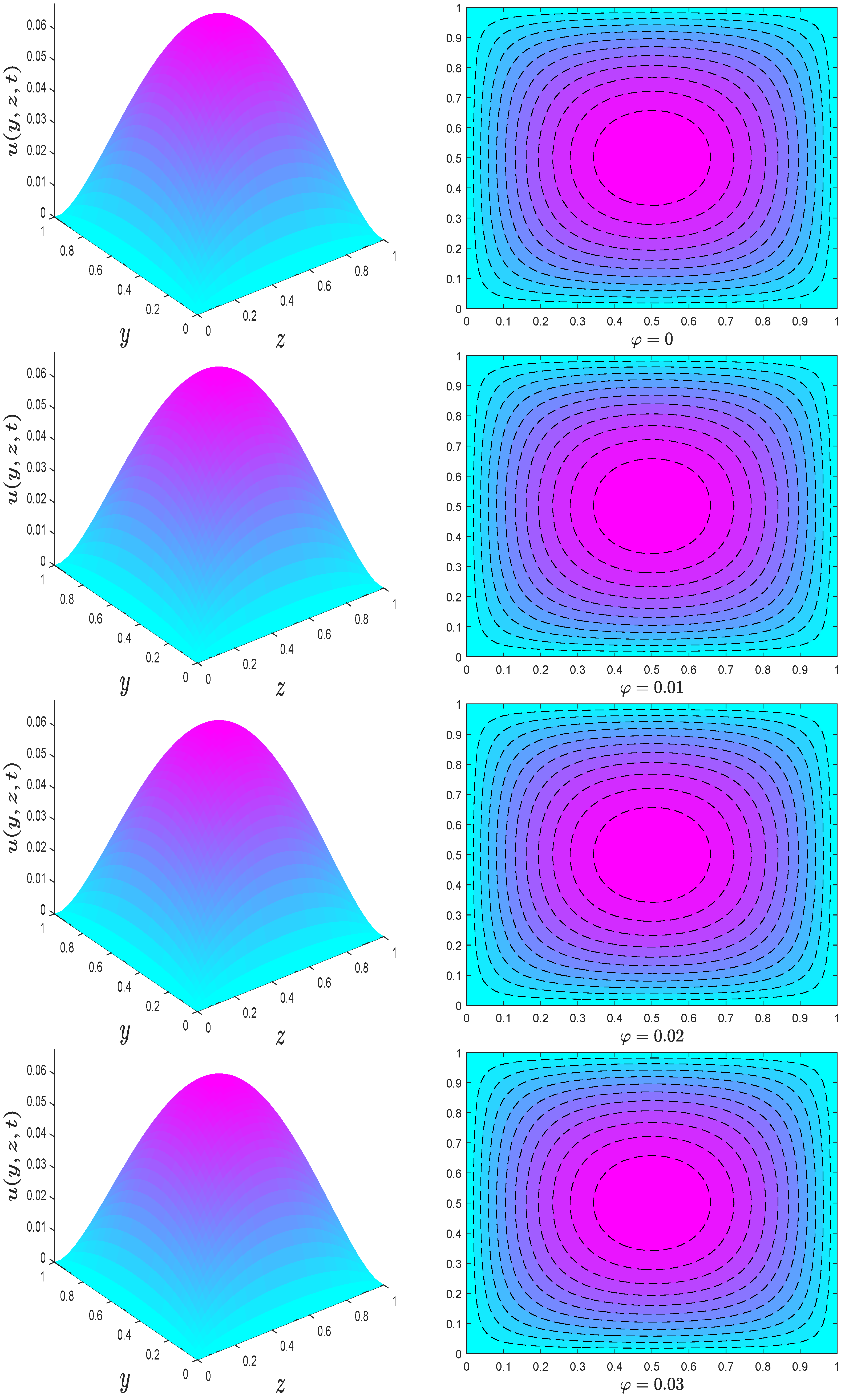
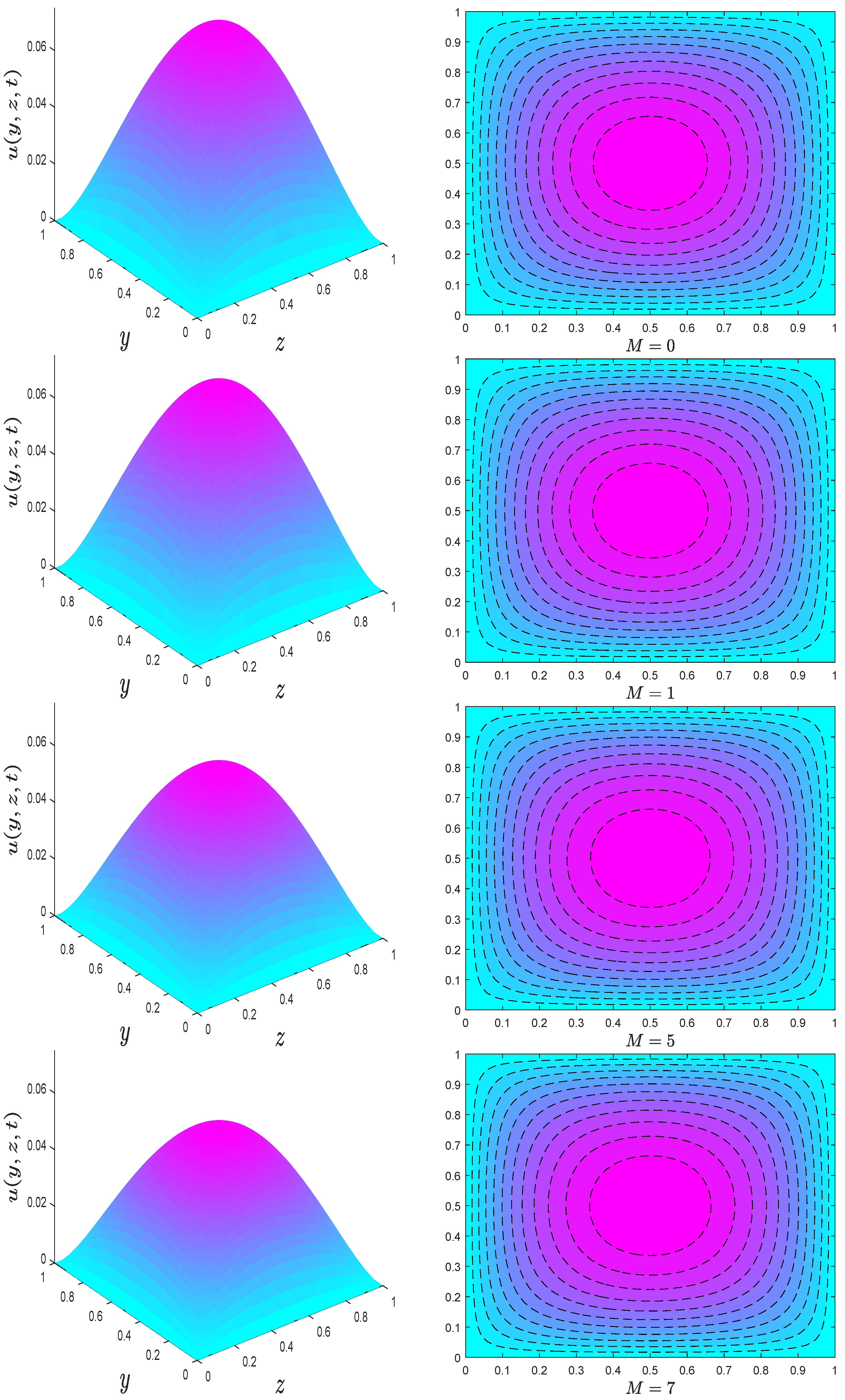
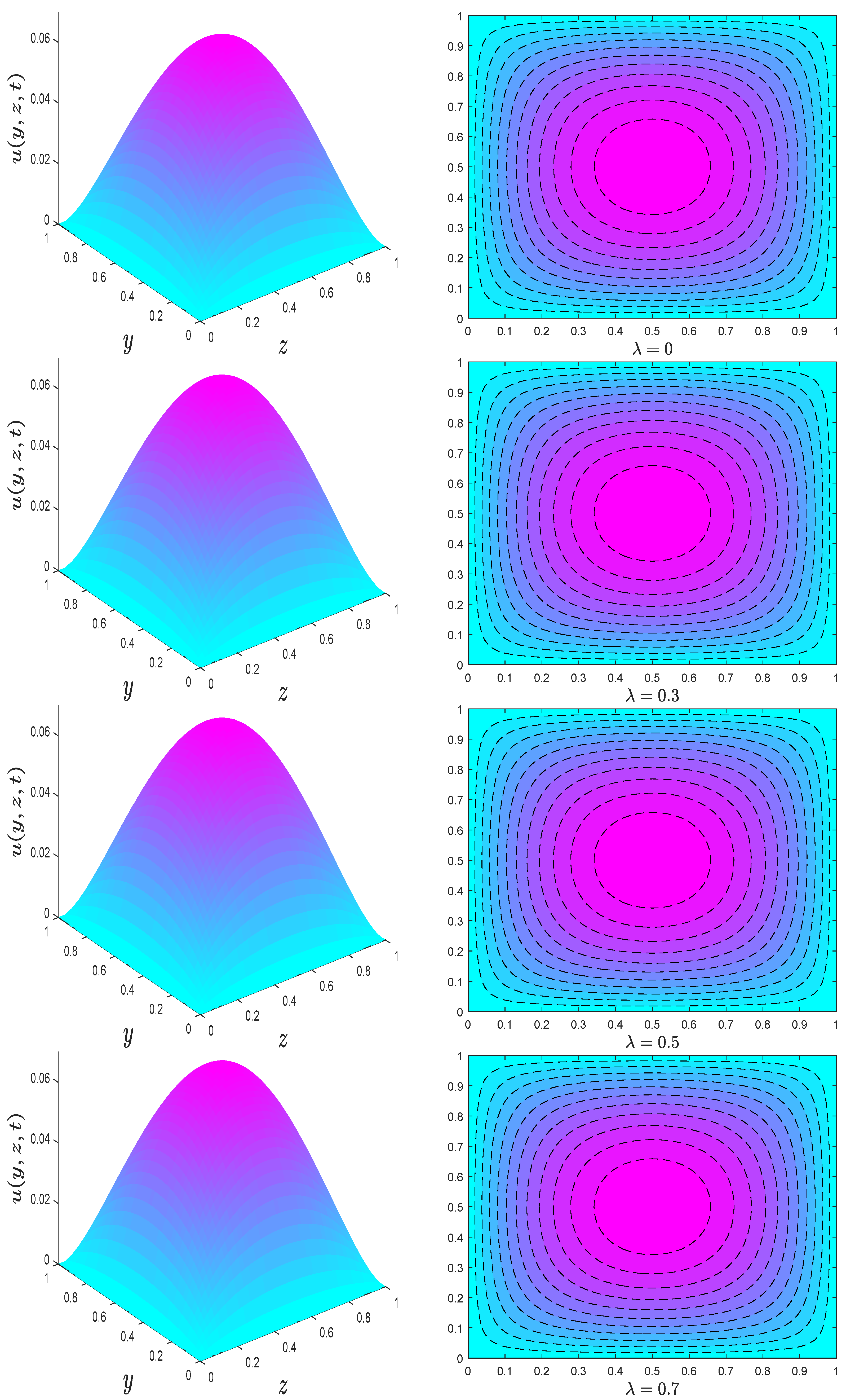
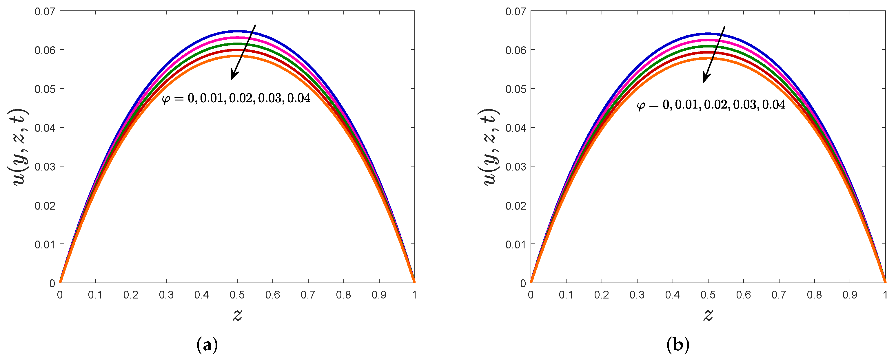
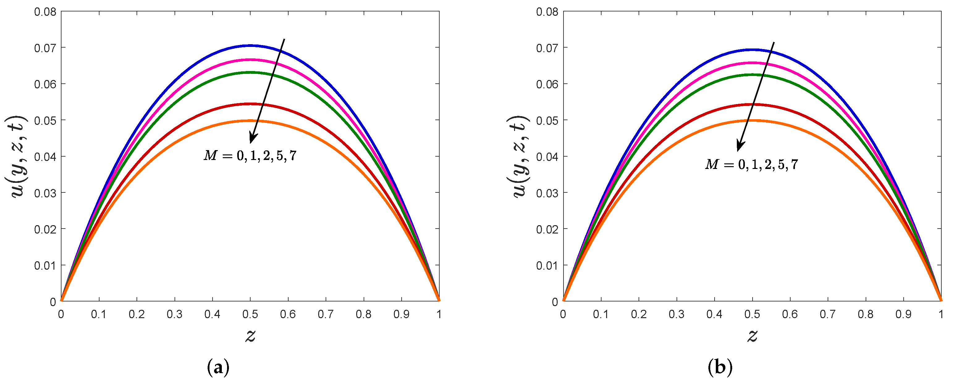
• Small values of the nanoparticle volume fraction and the magnetic parameter may often predict Maxwell fluid flow augmentation.
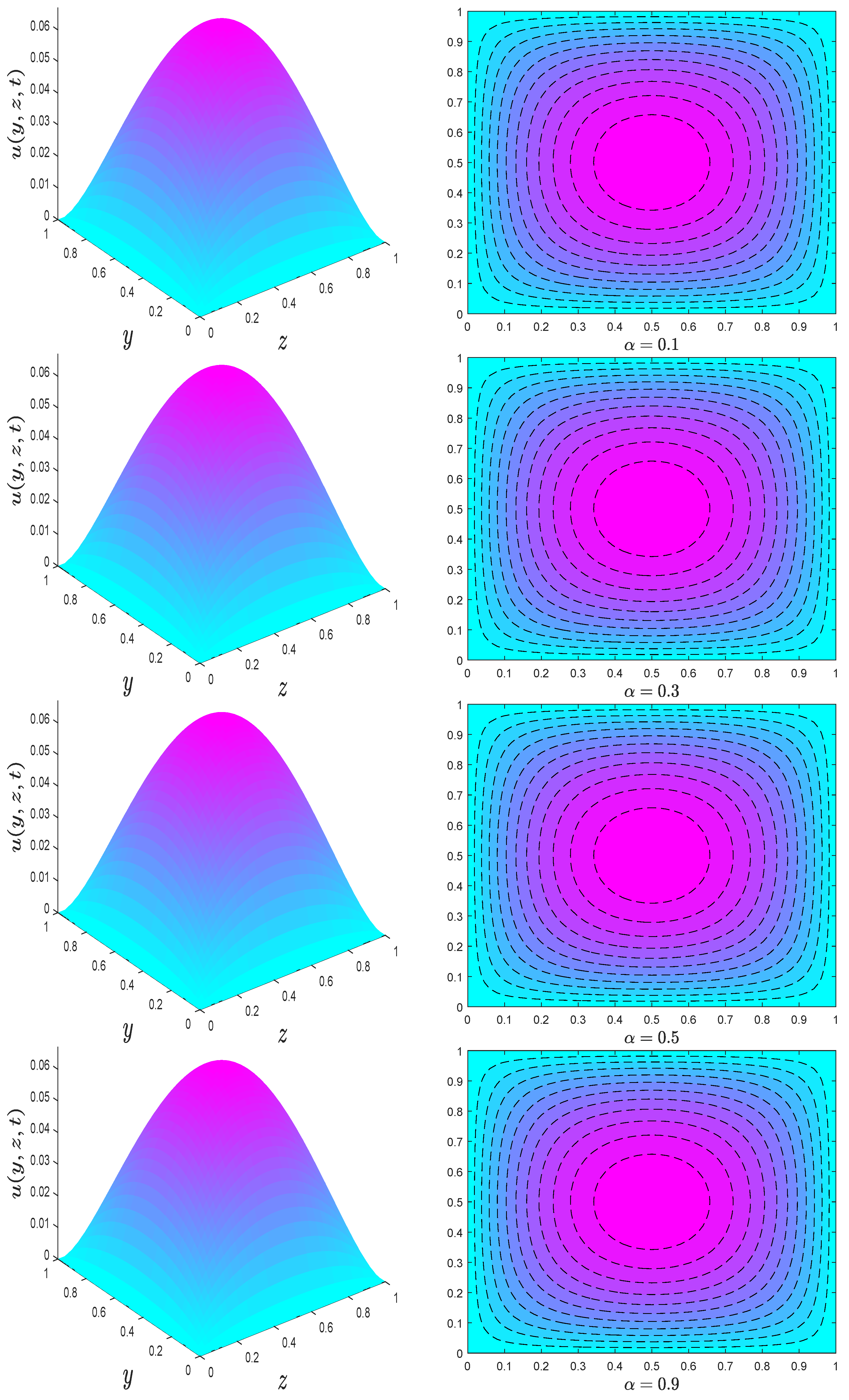
• The relaxation time parameter increases the amplitude of the velocity.
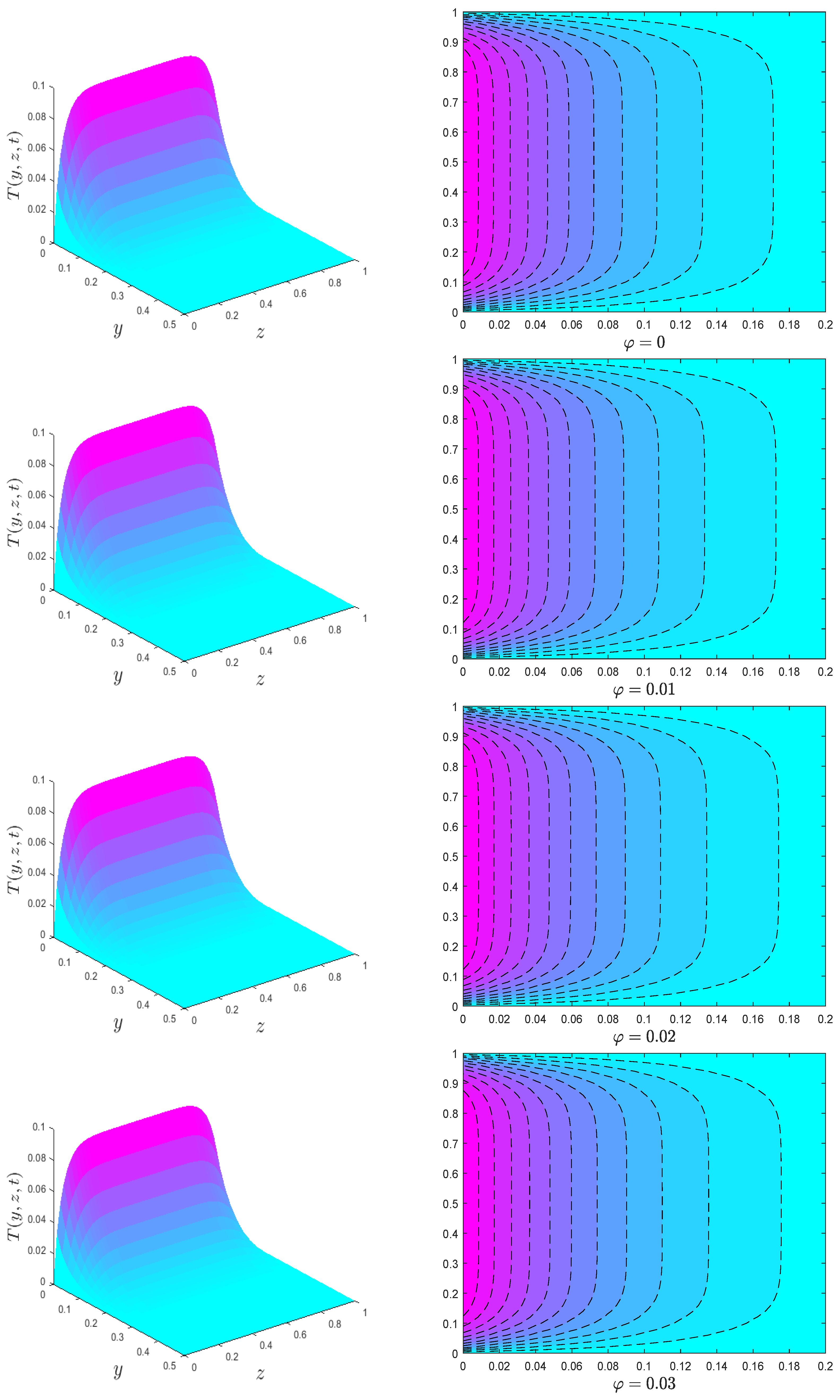
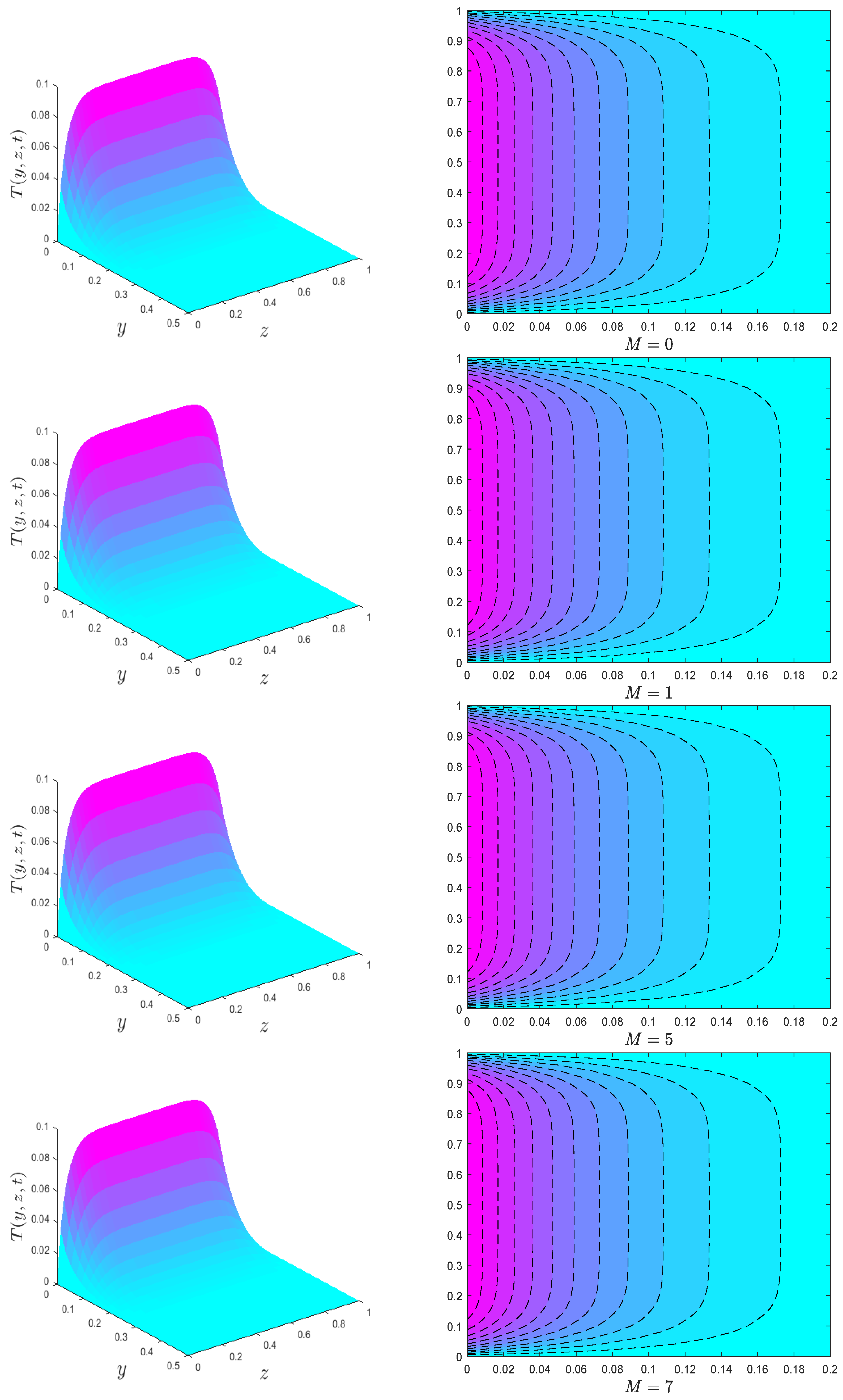
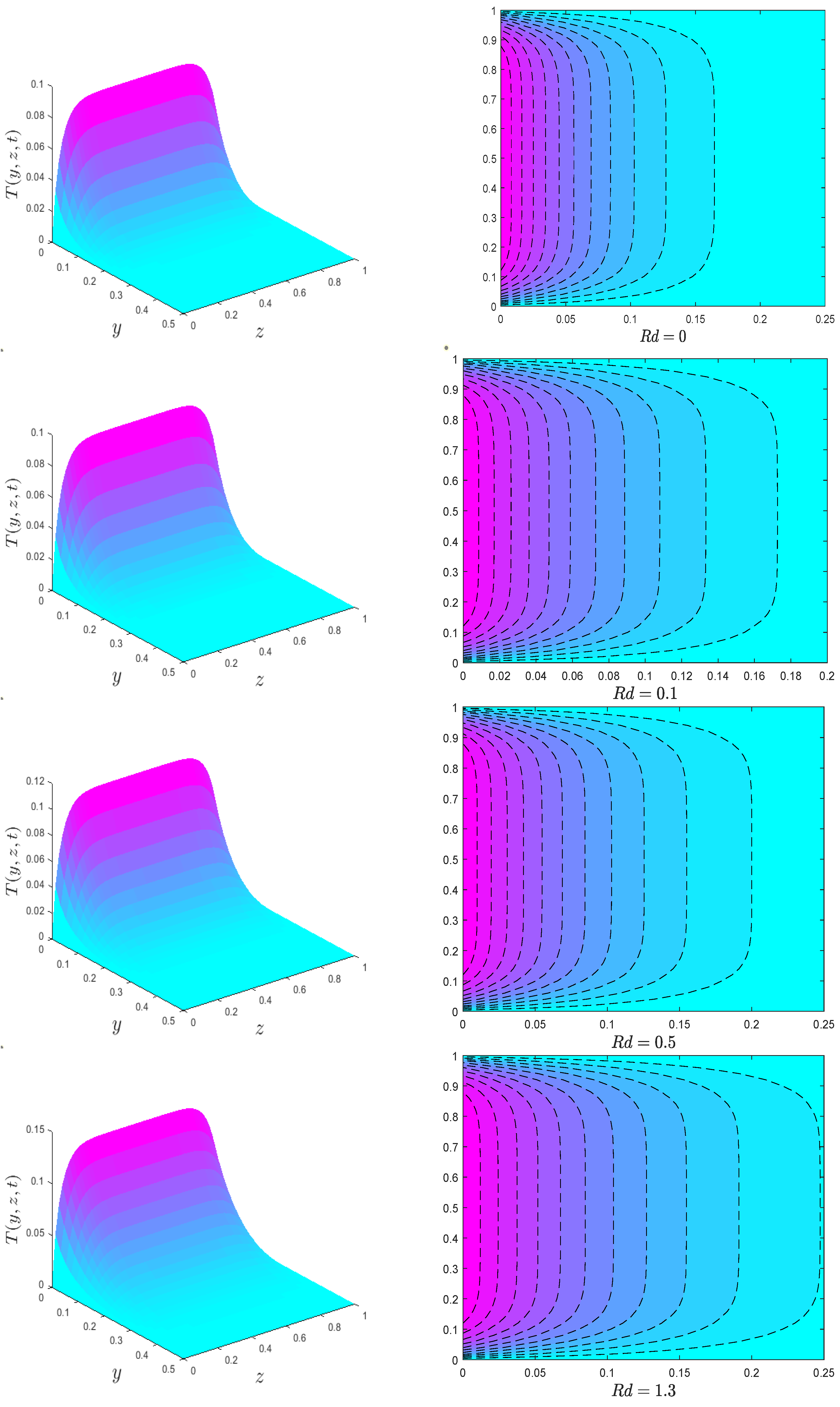
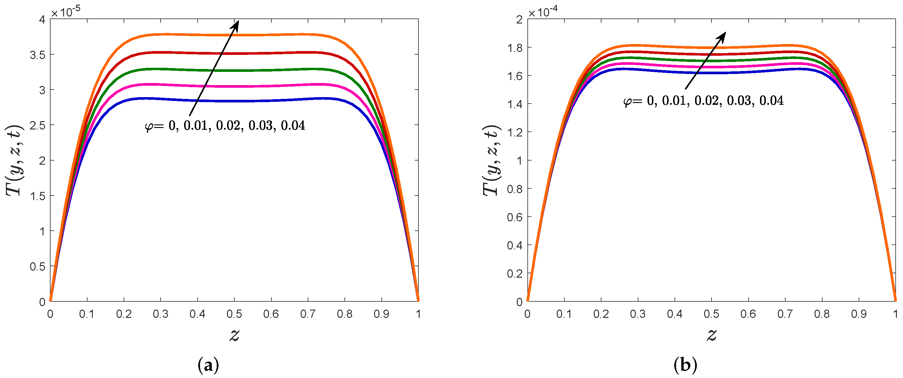
• To manifest a surface heat enhancement, the nanoparticle volume fraction, magnetic number, thermal radiation, and viscous dissipation parameters must all be substantial.

References

1. Feynman, R. There is plenty of room at the bottom: An invitation to enter a new field of physics. Presented at the Lecture at American Physical Society Meeting, Pasadena, CA, USA, 29 December 1959. [Google Scholar]
2. Salata, O.V. Applications of nanoparticles in biology and medicine. J. Nanobiotechnol. 2004, 2, 3. [Google Scholar] [CrossRef] [PubMed] [Green Version]
3. Masuda, H.; Ebata, A.; Teramae, K. Alteration of thermal conductivity and viscosity of liquid by dispersing ultra-fine particles. Dispersion of Al2O3, SiO2 and TiO2 ultra-fine particles. J-STAGE 1993, 7, 227–233. [Google Scholar] [CrossRef]
4. Choi, U.S.U.; Eastman, J.A. Enhancing thermal conductivity of fluids with nanoparticles. In Proceedings of the International Mechanical Engineering Congress and Exhibition, San Francisco, CA, USA, 12–17 November 1995. [Google Scholar]
5. Islam, T.; Yavuz, M.; Parveen, N.; Fayz-Al-Asad, M. Impact of Non-Uniform Periodic Magnetic Field on Unsteady Natural Convection Flow of Nanofluids in Square Enclosure. Fractal Fract. 2022, 6, 101. [Google Scholar] [CrossRef]
6. Wakif, A.; Boulahia, Z.; Ali, F.; Eid, M.R.; Sehaqui, R. Numerical analysis of the unsteady natural convection MHD Couette nanofluid flow in the presence of thermal radiation using single and two-phase nanofluid models for Cu–water nanofluids. Int. J. Appl. Comput. Math. 2018, 4, 81. [Google Scholar] [CrossRef]
7. Xia, W.-F.; Khan, M.I.; Khan, S.U.; Shah, F.; Khan, M.I. Dynamics of unsteady reactive flow of viscous nanomaterial subject to Ohmic heating, heat source and viscous dissipation. Ain Shams Eng. J. 2021, 12, 3997–4005. [Google Scholar] [CrossRef]
8. Hanif, H.; Khan, I.; Shafie, S.; Khan, W.A. Heat Transfer in Cadmium Telluride-Water Nanofluid over a Vertical Cone under the Effects of Magnetic Field inside Porous Medium. Processes 2020, 8, 7. [Google Scholar] [CrossRef] [Green Version]
9. Shi, Y.; Abidi, A.; Khetib, Y.; Zhang, L.; Sharifpur, M.; Cheraghian, G. The computational study of nanoparticles shape effects on thermal behavior of H2O-Fe nanofluid: A molecular dynamics approach. J. Mol. Liq. 2022, 346, 117093. [Google Scholar] [CrossRef]
10. Hanif, H. A finite difference method to analyze heat and mass transfer in kerosene based γ-oxide nanofluid for cooling applications. Phys. Scr. 2021, 96, 095215. [Google Scholar] [CrossRef]
11. Mallakpour, S.; Khadem, E. Recent development in the synthesis of polymer nanocomposites based on nano-alumina. Prog. Polym. Sci. 2015, 51, 74–93. [Google Scholar] [CrossRef]
12. Haridas, D.; Rajput, N.S.; Srivastava, A. Interferometric study of heat transfer characteristics of Al2O3 and SiO2-based dilute nanofluids under simultaneously developing flow regime in compact channels. Int. J. Heat Mass Transf. 2015, 88, 713–727. [Google Scholar] [CrossRef]
13. Animasaun, I.L. 47 nm alumina–water nanofluid flow within boundary layer formed on upper horizontal surface of paraboloid of revolution in the presence of quartic autocatalysis chemical reaction. Alex. Eng. J. 2016, 55, 2375–2389. [Google Scholar] [CrossRef] [Green Version]
14. Kabeel, A.; Abdelgaied, M. Study on the effect of alumina nano-fluid on sharp-edge orifice flow characteristics in both cavitations and non-cavitations turbulent flow regimes. Alex. Eng. J. 2016, 55, 1099–1106. [Google Scholar] [CrossRef] [Green Version]
15. Hawwash, A.; Abdel-Rahman, A.K.; Ookawara, S.; Nada, S. Experimental study of alumina nanofluids effects on thermal performance efficiency of flat plate solar collectors. J. Eng. Technol. (JET) 2016, 4, 123–131. [Google Scholar]
16. Sheikholeslami, M.; Ebrahimpour, Z. Thermal improvement of linear Fresnel solar system utilizing Al2O3-water nanofluid and multi-way twisted tape. Int. J. Therm. Sci. 2022, 176, 107505. [Google Scholar] [CrossRef]
17. Bahari, N.M.; Che Mohamed Hussein, S.N.; Othman, N.H. Synthesis of Al2O3–SiO2/water hybrid nanofluids and effects of surfactant toward dispersion and stability. Part. Sci. Technol. 2021, 39, 844–858. [Google Scholar] [CrossRef]
18. Ho, C.; Cheng, C.Y.; Yang, T.F.; Rashidi, S.; Yan, W.M. Cooling characteristics and entropy production of nanofluid flowing through tube. Alex. Eng. J. 2022, 61, 427–441. [Google Scholar] [CrossRef]
19. Denn, M.M. Fifty years of non-Newtonian fluid dynamics. AIChE J. 2004, 50, 2335–2345. [Google Scholar] [CrossRef]
20. Mackosko, C.W. Rheology: Principles, Measurements and Applications; VCH Publishers, Inc.: New York, NY, USA, 1994. [Google Scholar]
21. Adegbie, K.S.; Omowaye, A.J.; Disu, A.B.; Animasaun, I.L. Heat and mass transfer of upper convected Maxwell fluid flow with variable thermo-physical properties over a horizontal melting surface. Appl. Math. 2015, 6, 1362. [Google Scholar] [CrossRef] [Green Version]
22. Megahed, A.M. Improvement of heat transfer mechanism through a Maxwell fluid flow over a stretching sheet embedded in a porous medium and convectively heated. Math. Comput. Simul. 2021, 187, 97–109. [Google Scholar] [CrossRef]
23. Shafiq, A.; Khalique, C.M. Lie group analysis of upper convected Maxwell fluid flow along stretching surface. Alex. Eng. J. 2020, 59, 2533–2541. [Google Scholar] [CrossRef]
24. Hilfer, R. Applications of Fractional Calculus in Physics; World Scientific Publishing: Singapore, 2000. [Google Scholar] [CrossRef]
25. Meral, F.; Royston, T.; Magin, R. Fractional calculus in viscoelasticity: An experimental study. Commun. Nonlinear Sci. Numer. Simul. 2010, 15, 939–945. [Google Scholar] [CrossRef]
26. Yang, P.; Lam, Y.C.; Zhu, K.Q. Constitutive equation with fractional derivatives for the generalized UCM model. J. Non–Newton. Fluid Mech. 2010, 165, 88–97. [Google Scholar] [CrossRef]
27. Heymans, N. Hierarchical models for viscoelasticity: Dynamic behaviour in the linear range. Rheol. Acta 1996, 35, 508–519. [Google Scholar] [CrossRef]
28. Liu, L.; Feng, L.; Xu, Q.; Zheng, L.; Liu, F. Flow and heat transfer of generalized Maxwell fluid over a moving plate with distributed order time fractional constitutive models. Int. Commun. Heat Mass Transf. 2020, 116, 104679. [Google Scholar] [CrossRef]
29. Yang, W.; Chen, X.; Jiang, Z.; Zhang, X.; Zheng, L. Effect of slip boundary condition on flow and heat transfer of a double fractional Maxwell fluid. Chin. J. Phys. 2020, 68, 214–223. [Google Scholar] [CrossRef]
30. Razzaq, A.; Seadawy, A.R.; Raza, N. Heat transfer analysis of viscoelastic fluid flow with fractional Maxwell model in the cylindrical geometry. Phys. Scr. 2020, 95, 115220. [Google Scholar] [CrossRef]
31. Hanif, H. A computational approach for boundary layer flow and heat transfer of fractional Maxwell fluid. Math. Comput. Simul. 2022, 191, 1–13. [Google Scholar] [CrossRef]
32. Asjad, M.I.; Ali, R.; Iqbal, A.; Muhammad, T.; Chu, Y.M. Application of water based drilling clay-nanoparticles in heat transfer of fractional Maxwell fluid over an infinite flat surface. Sci. Rep. 2021, 11, 18833. [Google Scholar] [CrossRef]
33. Saqib, M.; Hanif, H.; Abdeljawad, T.; Khan, I.; Shafie, S.; Nisar, K.S. Heat transfer in mhd flow of maxwell fluid via fractional cattaneo-friedrich model: A finite difference approach. Comput. Mater. Contin 2020, 65, 1959–1973. [Google Scholar] [CrossRef]
34. Bayones, F.; Abd-Alla, A.; Thabet, E.N. Effect of heat and mass transfer and magnetic field on peristaltic flow of a fractional Maxwell fluid in a tube. Complexity 2021, 2021, 9911820. [Google Scholar] [CrossRef]
35. Podlubny, I. Fractional Differential Equations: An Introduction to Fractional Derivatives, Fractional Differential Equations, to Methods of Their Solution and Some of Their Applications; Academic Press: Cambridge, MA, USA, 1999. [Google Scholar]
36. Hanif, H. Cattaneo–Friedrich and Crank–Nicolson analysis of upper-convected Maxwell fluid along a vertical plate. Chaos Solitons Fractals 2021, 153, 111463. [Google Scholar] [CrossRef]
37. Davidson, P.A. An introduction to magnetohydrodynamics. Am. J. Phys. 2002, 70, 781. [Google Scholar] [CrossRef]
38. Fontes, D.H.; Ribatski, G.; Bandarra Filho, E.P. Experimental evaluation of thermal conductivity, viscosity and breakdown voltage AC of nanofluids of carbon nanotubes and diamond in transformer oil. Diam. Relat. Mater. 2015, 58, 115–121. [Google Scholar] [CrossRef]
39. Devi, S.A.; Devi, S.S.U. Numerical investigation of hydromagnetic hybrid Cu–Al2O3/water nanofluid flow over a permeable stretching sheet with suction. Int. J. Nonlinear Sci. Numer. Simul. 2016, 17, 249–257. [Google Scholar] [CrossRef]
Figure 1. Graphical representation of the flow model.
Fractalfract 06 00180 g001
Figure 2. Velocity profile for different values of nanoparticle volume fraction φ .
Fractalfract 06 00180 g002
Figure 3. Velocity profile for different values of magnetic parameter M.
Fractalfract 06 00180 g003
Figure 4. Velocity profile for different values of fractional derivative parameter α .
Fractalfract 06 00180 g004
Figure 5. Velocity profile for different values of relaxation time parameter λ .
Fractalfract 06 00180 g005
Figure 6. Temperature profile for different values of nanoparticle volume fraction φ .
Fractalfract 06 00180 g006
Figure 7. Temperature profile for different values of magnetic parameter M.
Fractalfract 06 00180 g007
Figure 8. Temperature profile for different values of thermal radiation parameter R d .
Fractalfract 06 00180 g008
Figure 9. Temperature profile for different values of dissipation parameter E .
Fractalfract 06 00180 g009
Figure 10. One-dimensional velocity profile for various values of φ . (a) Maxwell fluid, (b) Newtonian fluid.
Fractalfract 06 00180 g010
Figure 11. One-dimensional velocity profile for various values of M. (a) Maxwell fluid, (b) Newtonian fluid.
Fractalfract 06 00180 g011
Figure 12. One-dimensional temperature profile for various values of φ . (a) Maxwell fluid, (b) Newtonian fluid.
Fractalfract 06 00180 g012
Figure 13. One-dimensional temperature profile for various values of E . (a) Maxwell fluid, (b) Newtonian fluid.
Fractalfract 06 00180 g013