Switched Fractional Order Multiagent Systems Containment Control with Event-Triggered Mechanism and Input Quantization

Abstract

This paper studies the containment control problem for a class of fractional order nonlinear multiagent systems in the presence of arbitrary switchings, unmeasured states, and quantized input signals by a hysteresis quantizer. Under the framework of the Lyapunov function theory, this paper proposes an event-triggered adaptive neural network dynamic surface quantized controller, in which dynamic surface control technology can avoid “explosion of complexity” and obtain fractional derivatives for virtual control functions continuously. Radial basis function neural networks (RBFNNs) are used to approximate the unknown nonlinear functions, and an observer is designed to obtain the unmeasured states. The proposed distributed protocol can ensure all the signals remain semi-global uniformly ultimately bounded in the closed-loop system, and all followers can converge to the convex hull spanned by the leaders’ trajectory. Utilizing the combination of an event-triggered scheme and quantized control technology, the controller is updated aperiodically only at the event-sampled instants such that transmitting and computational costs are greatly reduced. Simulations compare the event-triggered scheme without quantization control technology with the control method proposed in this paper, and the results show that the event-triggered scheme combined with the quantization mechanism reduces the number of control inputs by 7% to 20%.

1. Introduction

Multiagent systems (MASs) cooperative control technology has been widely used in many fields [1,2,3,4]. As the most basic research content of multiagent cooperative control, the consensus problem has made much progress [5,6,7,8,9,10,11]. Further study of the cooperative control problem of multiagent systems, extending the consensus control of a single leader, considers multiagent cooperative control in the case of multiple leaders, and designs a controller to make the followers converge to a convex hull composed of multiple leaders, which is called containment control. As a special case of cooperative control, many research results of MASs containment control have been reported in the field of integer order control, such as adaptive control [12,13], feedback control [14,15], linear matrix inequalities (LMIs) [16,17], sliding mode control [18], and so on.

Due to the unique memory properties of fractional calculus and the ability to accurately model the system, fractional calculus is suitable for describing real physical systems with genetics [19,20]. At present, the Caputo fractional differential definition is widely used in engineering, and there have been many achievements on the fractional derivative definition and control research of fractional order nonlinear systems. For example, Ref. [21] studied the numerical approximation for the spread of the SIQR model with a Caputo fractional derivative. Ref. [22] expanded the garden equation to the Caputo derivative and Atangana-Baleanu fractional derivative in the sense of Caputo. Ref. [23] established the Caputo fractional derivatives for exponential s-convex functions. Some new k-Caputo fractional derivative inequalities were established in [24] by using Hermite-Hadamard-Mercer type inequalities for differentiable mapping. Ref. [25] proposed two fractional derivatives by taking the Caputo fractional derivative and replacing the simple derivative with a proportional type derivative, which can be expressed as a combination of existing fractional operators in several different ways. In order to perform reliable and effective numerical processing of nonlinear singular fractional Lane-Emden differential equations, based on fractional Meyer wavelet artificial neural network optimization, combined with the comprehensive strength of genetic algorithm-assisted active set method, Ref. [26] proposed a stochastic calculation solver fractional Meyer Wavelet Artificial Neural Network Genetic Algorithm and Active Sets. In reference [27], the authors studied variable order fractional order and constant order fractional order systems with uncertain and external disturbance terms and proposed a variable order fractional control method for tracking control.

At present, the research into the multiagent systems containment control problem has made some progress in the field of fractional order systems. In reference [28], the authors applied the matrices singular value decomposition and LMI techniques for obtaining sufficient conditions to solve the containment problem of fractional order multiagent systems (FOMASs). In reference [29], the authors considered the distributed containment control problem for FOMASs with a double-integrator and designed a distributed projection containment controller for each follower. Due to the general approximation theory of the neural network (NN) and fuzzy logic system, it is often used to deal with the uncertainty of nonlinear systems to obtain unknown nonlinear functions [30]. For example, based on the neural network algorithm, reference [31] designed a distributed control algorithm to ensure that the follower converged to the leader signal in FOMASs. For the FOMASs containment control, an adaptive NN containment controller was designed in reference [12], in which RBFNNs were applied for the unknown functions. In most practical applications, it is usually necessary to obtain the unmeasurable state of the system through a state observer. For example, reference [32] designed a state observer to provide an estimate for unmeasured consensus errors and disturbances of FOMASs. Reference [33] designed an observer to obtain the state of the agent for FOMASs containment control. It should be recognized that the abovementioned fractional order nonlinear system is a kind of non-switched system, and the switched system is another more complex system, which is composed of multiple subsystems and is formed by signal switching between the systems. For the switched system, when switching between subsystems, the system parameters will change greatly, and the nonlinear function of its system will become discontinuous, so the performance of the system may be affected or even unstable [34]. Therefore, it is well worth investigating how to obtain conditions that make the switching system stable for all switching signals. Reference [35] studied the stability and robust stabilization of switched fractional order systems and provided two stability theorems for switched fractional order systems under the arbitrary switching. Based on the fractional Lyapunov stability criterion, reference [36] designed an adaptive fuzzy controller for the uncertain fractional-order switched nonlinear systems and ensured that the tracking error converged to a small neighborhood of the origin regardless of arbitrary switching. The switching control method for strictly feedback switched nonlinear systems was studied by using the average dwell time method in references [37,38].

The traditional time sampling mechanism will cause unnecessary waste of communication resources. In modern technology, an event-triggered mechanism and quantized mechanism can reduce the action frequency of the controller, thus overcoming the problem of wasting communication resources [39]. For example, reference [40] solved the problem of event-triggered fuzzy adaptive tracking control for MASs with input quantization and reduced the communication burden by combining an asymmetric hysteresis quantizer and event triggering mechanism. Based on quantized feedback control, Reference [41] studied the problem of adaptive event-triggered tracking for nonlinear systems with external disturbances. In reference [42], the authors designed an adaptive neural control scheme for integer order uncertain nonlinear systems by combining an event-triggered scheme with input quantization technology. For the containment problem of MASs with unmeasured states, reference [43] developed a quantized control scheme based on the event-triggered backstepping control technique. To the best of our knowledge, the containment control problem of switched fractional order multiagent systems (SFOMAS) combining an event-triggered mechanism and input quantization techniques has not been studied, which motivates the research presented in this paper. Furthermore, the combination of the event-triggered mechanism and the input quantification can reduce the operating frequency of the actuation system and thus reduce energy consumption. Therefore, the research in this paper has great value in the practical engineering application of MASs and reducing the fatigue loss in the system.

Based on the previous discussion, this paper designs an observer-based event-triggered adaptive neural network dynamic surface quantized controller to addresses the containment control of SFOMASs. Compared with the previous research work, the main contributions of the control method discussed in this paper are summarized as follows.

(1) Comparison with [34,37,38], an adaptive neural network dynamic surface controller is proposed to address the containment control problem of SFOMASs, in which the controller combines the event-triggered mechanism and input quantization to reduce controller action frequency in this paper.

(2) Compared with references [38,40], the state observer is used to estimate system states, and the RBFNN is developed to estimate uncertain parts. In comparison with references [41,43], fractional order DSC technology is used to avoid the “explosion of complexity” that can occur during traditional backstepping design processes and to obtain fractional derivatives for virtual control continuously.

The rest of the paper is organized as follows. Section 2 introduces basic theory about fractional calculus and SFOMASs. In Section 3, first, we construct an observer to estimate the system state, then a controller is proposed based on the adaptive dynamic surface control method; finally, the stability is proved by the Lyapunov function theory. Section 4 provides the numerical simulations to show the viability and efficiency of the proposed controller. Section 5 offers conclusions.

2. Preliminaries

2.1. Fractional Calculus

The Caputo fractional derivative [44] is defined as

$$\begin{array}{c}\hfill {}_0^C{D}_t^{\alpha }f\left(t\right)=\frac{1}{\Gamma \left(n-\alpha \right)}{\int }_0^t\frac{f^{\left(n\right)}\left(\tau \right)}{{\left(t-\tau \right)}^{1+\alpha -n}}d\tau ,\end{array}$$

where $n\in N$ and $n-1<\alpha \le n$, $\Gamma \left(z\right)={\int }_0^{\infty }{t}^{z-1}{e}^{-t}dt$ is the Gamma function.

Lemma 1

([45]). For a complex number β and two real numbers $\alpha ,v$ satisfying $\alpha \in \left(0,1\right)$ and

$$\begin{array}{c}\hfill \frac{\pi \alpha }{2}<vs.<min\left\{\pi ,\pi \alpha \right\}\end{array}$$

For all integers $n\ge 1$, we can obtain

$$\begin{array}{c}\hfill E_{\alpha ,\beta }\left(\varsigma \right)=-\sum _{j=1}^{\infty }\frac{1}{\Gamma \left(\beta -\alpha j\right)}+o\left(\frac{1}{{\left|\varsigma \right|}^{n+1}}\right)\end{array}$$

when $\left|\varsigma \right|\to \infty ,v\le \left|arg\left(\varsigma \right)\right|\le \pi$.

Lemma 2

([45]). If v satisfies the condition of Lemma 1, then the following inequality relation holds

$$\begin{array}{c}\hfill \left|E_{\alpha ,\beta }\left(\varsigma \right)\right|\le \frac{\mu }{1+\left|\varsigma \right|}\end{array}$$

where $\alpha \in \left(0,2\right)$ and β is an arbitrary real number, $\mu >0$, $\upsilon \le \left|arg\left(\varsigma \right)\right|\le \pi$, and $\left|\varsigma \right|\ge 0$.

Lemma 3

([46]). Let $x\left(t\right)\in R^l$ be a vector of differentiable function. Then, the following inequality holds

$$\begin{array}{c}\hfill \begin{array}{c}{D}^{\alpha }\left(x^T\left(t\right)Px\right)\le 2x^T\left(t\right)P{D}^{\alpha }x\left(t\right)\hfill \end{array}\end{array}$$

where $\alpha \in \left(0,1\right)$ and P is a positive definite diagonal matrix.

Lemma 4

([47]). (Young’s inequality) For any $x,y\in R^n$, the following inequality relationship holds

$$\begin{array}{c}\hfill x^{T}y\le \frac{c^a}{a}{∥x∥}^a+\frac{1}{b{c}^b}{∥y∥}^b\end{array}$$

where $a>1,b>1,c>0$, and $\left(a-1\right)\left(b-1\right)=1$.

Lemma 5

([48]). For $m\in R$ and $n>0$, the following inequality holds

$$\begin{array}{c}\hfill 0\le \left|m\right|-\frac{m^2}{\sqrt{m^2+n^2}}\le n\end{array}$$

Lemma 6

([44]). Suppose that the Lyapunov function $V\left(t,x\right)$ satisfies $D^{\alpha }V\left(t,x\right)\le -CV\left(t,x\right)$$+D$. Let $0<\alpha <1$, $C>0$ and $D\ge 0$, the following inequality holds

$$\begin{array}{c}\hfill \begin{array}{cc}V\left(t,x\right)\le V\left(0\right)E_{\alpha }\left(-C{t}^{\alpha }\right)+\frac{D\mu }{C},& t\ge 0\end{array}\end{array}$$

Then, $V\left(t,x\right)$ is bounded on $\left[0,t\right]$ and fractional order systems are stable, where μ is defined in Lemma 2.

2.2. Problem Formulation

In the paper, we consider the following fractional order multiagent system.

$$\left\{\begin{array}{cc}\hfill D^{\alpha }{x}_{i,1}\left(t\right)& =x_{i,2}+f_{i,1}^{\sigma \left(t\right)}\left(x_{i,1}\right)\hfill \\ \hfill D^{\alpha }{x}_{i,l}\left(t\right)& =x_{i,l+1}+f_{i,l}^{\sigma \left(t\right)}\left(x_{i,1},x_{i,2},\dots ,x_{i,l}\right)\hfill \\ \hfill D^{\alpha }{x}_{i,n}\left(t\right)& =u_i\left(t\right)+f_{i,n}^{\sigma \left(t\right)}\left(x_{i,1},x_{i,2},\dots ,x_{i,n}\right)\hfill \\ \hfill y_i& =x_{i,1}\hfill \end{array}\right.$$

(1)

where $l=2,\dots ,n-1$, $\alpha \in \left(0,1\right)$; $X_{i,l}={\left(x_{i,1},x_{i,2},\dots ,x_{i,l}\right)}^T$$\in R^l$ are the system state vectors, and $u_i\left(t\right)$ is the control input of the system. It should be noted that the control input in this paper considers the quantization mechanism and the event-triggered technology. $y_i$ is the system output, and $f_{i,l}^{\sigma \left(t\right)}\left(x_{i,1},x_{i,2},\dots ,x_{i,l}\right)$ are unknown nonlinear functions. $\sigma \left(t\right)$ is a piecewise continuous function that is used to describe the triggering conditions for switching between subsystems. It is called a switching signal, for example, if $\sigma \left(t\right)=q$, it means that $q-th$ subsystem is activated.

Rewriting system (1):

$$D^{\alpha }{X}_i=A_i{X}_i+K_i{y}_i+\sum _{l=1}^n{B}_{i,l}\left[f_{i,l}^q\left(X_{i,l}\right)\right]+B_i{u}_i\left(t\right)$$

(2)

where $A_i=\left[\begin{array}{c}-k_{i,1}\\ ⋮\\ -k_{i,n}\end{array}\begin{array}{ccc}& & \\ & I_{n-1}& \\ 0& \dots & 0\end{array}\right]$, $K_i=\left[\begin{array}{c}{k}_{i,1}\\ ⋮\\ k_{i,n}\end{array}\right]$, $B_i=\left[\begin{array}{c}0\\ ⋮\\ 1\end{array}\right]$, $B_{i,l}={\left[0\dots 1\dots 0\right]}^T$, and given a positive matrix $Q_i^T=Q_i$, there exists a positive matrix $P_i^T=P_i$ satisfying

$$A_i^T{P}_i+P_i{A}_i=-2Q_i$$

(3)

Control objectives: This paper aims to design an observer-based adaptive neural network dynamic surface controller, so that all the signals remain bounded in the closed-loop system and enable all followers to converge to the leaders’ convex hull. Meanwhile, we utilize the combination of an event-triggered scheme and quantized mechanism to reduce the transmission frequency of the control input.

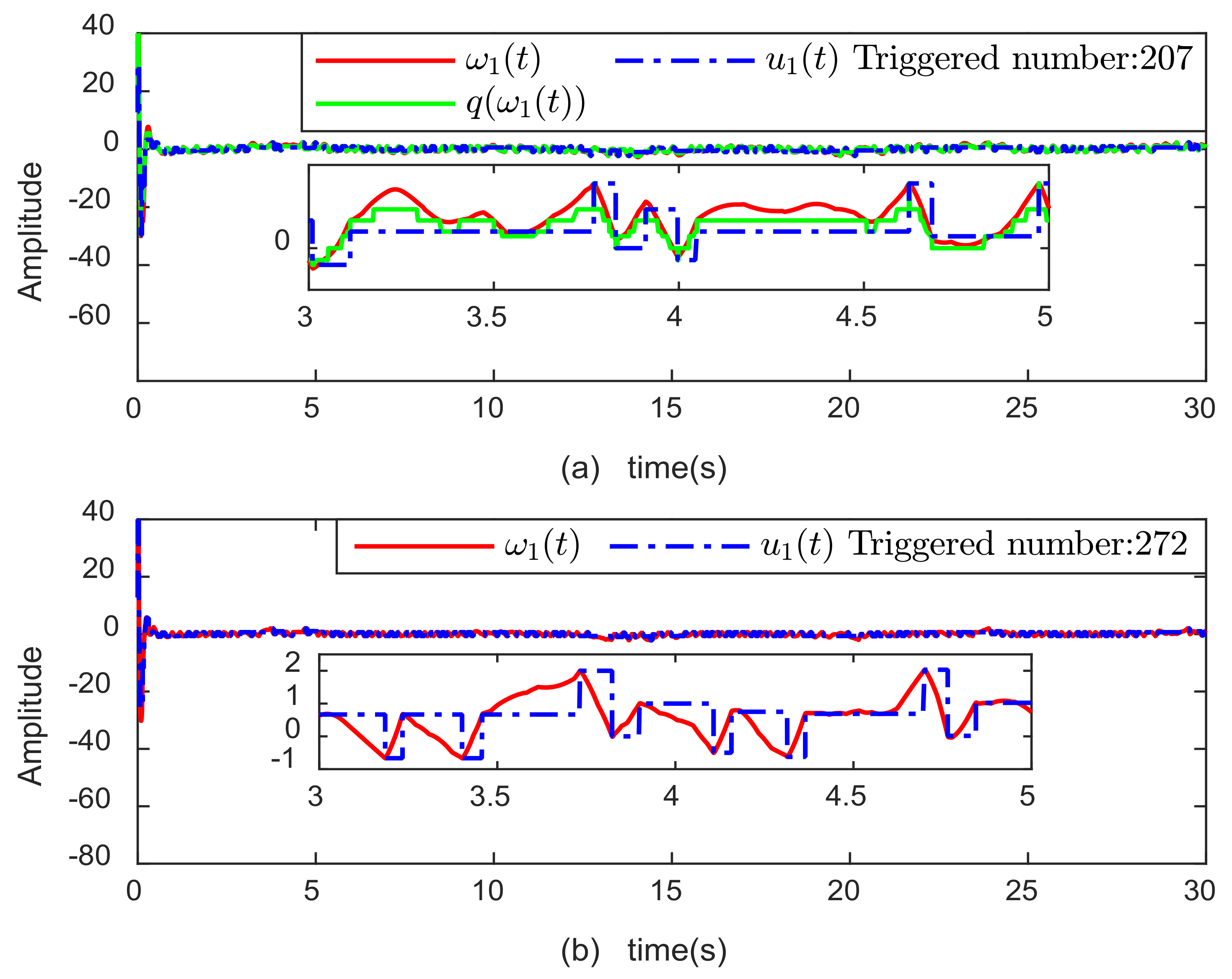
2.3. Hysteresis Quantizer

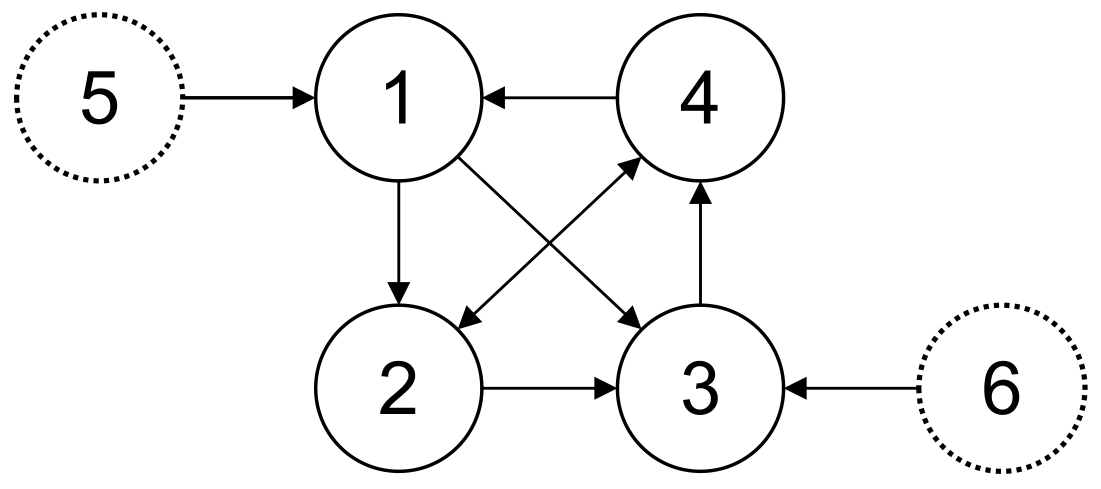
In this paper, the hysteresis quantizer is used to reduce chattering. The quantizer $q_i\left({\omega }_i\left(t\right)\right)$ is shown as the following form [49].

$$q_i\left({\omega }_i\left(t\right)\right)=\left\{\begin{array}{c}{\omega }_{is}sign\left({\omega }_i\right),\hfill \\ {\omega }_{is}\left(1+d\right)sign\left({\omega }_i\right),\hfill \\ 0,\hfill \end{array}\right.\begin{array}{c}\frac{{\omega }_{is}}{1+d}<\left|{\omega }_i\right|\le \frac{{\omega }_{is}}{1-d}\\ {\omega }_{is}<\left|{\omega }_i\right|\le \frac{{\omega }_{is}\left(1+d\right)}{1-d}\\ 0\le \left|{\omega }_i\right|<{\omega }_{min}\end{array}$$

(4)

where ${\omega }_{is}=n^{1-s}{\omega }_{min}\left(s=1,2,\dots \right)$ with parameters ${\omega }_{\min }>0$ and $0<n<1$, $d=\frac{1-n}{1+n}$. Meanwhile, $q_i\left({\omega }_i\left(t\right)\right)$ is in the set $U=\left[0,\pm {\omega }_{is},\pm {\omega }_{is}\left(1+d\right)\right],ands=1,2,\dots$. ${\omega }_{min}$ determines the magnitude of the dead-zone for $q_i\left({\omega }_i\left(t\right)\right)$.

Lemma 7

([49]). The system inputs $q_i\left({\omega }_i\left(t\right)\right)$ can be described as

$$q_i\left({\omega }_i\left(t\right)\right)=H\left({\omega }_i\right){\omega }_i\left(t\right)+L_i\left(t\right)$$

(5)

where $1-d\le H\left({\omega }_i\right)\le 1+d$,$\left|L\left(t\right)\right|\le {\omega }_{min}$.

2.4. Graph Theory

Suppose that there exist N followers, labeled as agents 1 to N, and M leaders, labeled as agents $N+1$ to $N+M$. The information exchange between followers is represented by a directed graph $G=\left(w,\epsilon ,\overline{A}\right)$, in which $w=\left\{n_1,\dots ,n_{N+M}\right\}$. The set of edge is exhibited as $\epsilon =\left\{\left(n_i,n_j\right)\right\}\in w\times w$, which expresses that follower i and follower j can exchange information, and $N_i=\left\{j\left|\left(n_i,n_j\right)\in \epsilon \right.\right\}$ means the neighbor set of followers i. Furthermore, $\overline{A}=\left\{a_{ij}\right\}\in R^{\left(N+M\right)\times \left(N+M\right)}$ is the Adjacency matrix, $a_{ij}$ of $\overline{A}$ is represented as if $\left(n_i,n_j\right)\notin \epsilon$, $a_{ij}=0$; if not, $a_{ij}=1$. It is supposed that $a_{ij}=0$. A directed graph G has a spanning tree if there exists at least one node called a root node, which has a directed path to all the other nodes. Define the Laplacian matrix $L=D-\overline{A}\in R^{\left(N+M\right)\times \left(N+M\right)}$ and the diagonal matrix $D=diag\left(d_1,\dots ,d_{N+M}\right)$, in which $d_i={\sum }_{j=1}^{N+M}{a}_{ij}$.

Suppose that leaders $N+1,\dots ,N+M$ do not receive the information from followers and other leaders, and the followers $1,\dots ,N$ have at least one neighbor. Therefore, the Laplacian matrix L related to directed communication graph G is described as follows:

$$\begin{array}{c}\hfill L=\left[\begin{array}{cc}{L}_1& L_2\\ 0_{M\times N}& 0_{M\times M}\end{array}\right]\end{array}$$

where $L_1\in R^{N\times N}$ is the matrix related to the communication between the N followers, and $L_2\in R^{N\times M}$ is the communication from M leaders to N followers. Let $r\left(t\right)={\left[r_{N+1},r_{N+2},\dots ,r_{N+M}\right]}^T$, and $Co\left(r\left(t\right)\right)=\left\{{\sum }_{j=N+1}^{N+M}{\theta }_j{r}_j\left|r_j\in r\left(t\right),{\theta }_j>0,{\sum }_{j=N+1}^{N+M}{\theta }_j=1\right.\right\}$. Define the convex hull as $r_d\left(t\right)={\left[r_{d,1}\left(t\right),r_{d,2}\left(t\right),\dots ,r_{d,M}\left(t\right)\right]}^T$$=-L_1^{-1}{L}_{2}r\left(t\right)$. The containment errors are defined as $e_i=y_i-r_{d,i}$. Let $e={\left[e_1,e_2,\dots ,e_N\right]}^T$, $y={\left[y_1,y_2,\dots ,y_N\right]}^T$, then $e=y-r_d\left(t\right)$.

2.5. Neural Network Approximation

Due to its universal approximation characteristics, neural networks have been widely used in the identification and control of uncertain nonlinear systems [10]. In this paper, we employ an RBFNNs to identify the nonlinear functions. The unknown function $f\left(Z\right)$ can be expressed as

$$\begin{array}{c}\hfill f_{nn}\left(Z\right)={\theta }^T\phi \left(Z\right)\end{array}$$

where $\theta$ is the weight vector and $\phi \left(Z\right)$ is the basis function vector. In this paper, due to applying radial basis function neural networks (RBFNNs), Gaussian basis functions are used. For any unknown function $f\left(Z\right)$ defined over a compact set U, there exists the neural network ${\theta }^{*T}\phi \left(Z\right)$ and arbitrary accuracy $\epsilon \left(Z\right)$ such that

$$\begin{array}{c}\hfill f\left(Z\right)={\theta }^{*T}\phi \left(Z\right)+\epsilon \left(Z\right)\end{array}$$

where ${\theta }^{*}$ is the vectors of optimal parameters defined by ${\theta }^{*}=arg{min}_{\theta \in \Omega }\left[{sup}_{Z\in U}\left|f\left(Z\right)-{\theta }^T\phi \left(Z\right)\right|\right]$, and $\epsilon \left(Z\right)$ denotes the minimum approximation error.

Assumption 1.

The optimal approximation errors remain bounded, there exists a positive constant ${\epsilon }_0$, satisfying $\left|\epsilon \left(Z\right)\right|\le {\epsilon }_0$.

3. Main Results

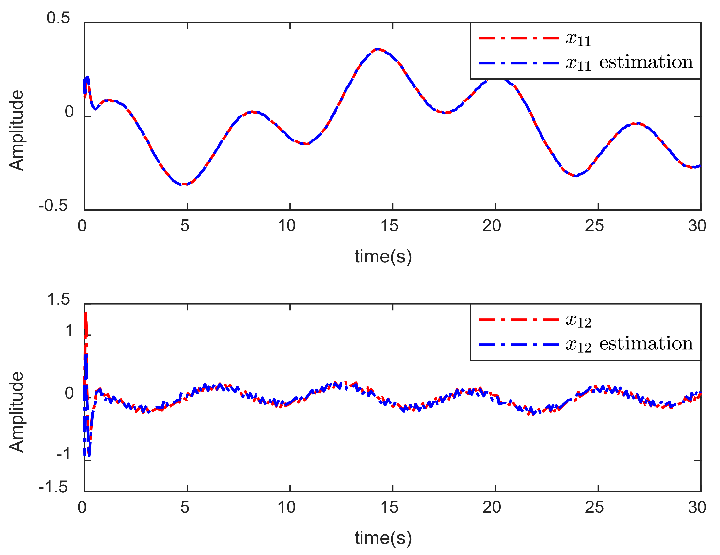
3.1. Observer Design

Assumption 2.

In this paper, we employ neural networks to identify the nonlinear functions. The unknown functions $f_i\left(X\right)$, $i=1,\dots ,n$ can be expressed as

$$f_i\left(X_i\left|{\theta }_i\right.\right)={\theta }_i^T{\phi }_i\left(X_i\right),1\le i\le n.$$

(6)

Furthermore, we assume that the state variables of system (1) are not available. The state observer is designed as follows:

$$\begin{array}{cc}\hfill D^{\alpha }{\widehat{X}}_i& =A_i{\widehat{X}}_i+K_i{y}_i+\sum _{l=1}^n{B}_{i,l}{\widehat{f}}_{i,l}^q\left({\widehat{X}}_{i,l}\left|{\theta }_{i,l}\right.\right)+B_i{u}_i\left(t\right)\hfill \\ \hfill {\widehat{y}}_i& =C_i{\widehat{X}}_i\hfill \end{array}$$

(7)

where $C_i=\left[1\dots 0\dots 0\right]$, and ${\widehat{X}}_{i,l}={\left({\widehat{x}}_{i,1},{\widehat{x}}_{i,2},\dots ,{\widehat{x}}_{i,l}\right)}^T$ are the estimated values of $X_{i,l}={\left(x_{i,1},x_{i,2},\dots ,x_{i,l}\right)}^T$.

We define $e_i=X_i-{\widehat{X}}_i$ as the observation error, and then, according to Equations (2) and (6), one has

$$\begin{array}{c}\hfill D^{\alpha }{e}_i=A_i{e}_i+\sum _{l=1}^n{B}_{i,l}\left[f_{i,l}^q\left({\widehat{X}}_{i,l}\right)-{\widehat{f}}_{i,l}^q\left({\widehat{X}}_{i,l}\left|{\theta }_{i,l}\right.\right)+\Delta f_{i,l}^q\right]\end{array}$$

(8)

where $\Delta f_{i,l}^q=f_{i,l}^q\left(X_{i,l}\right)-f_{i,l}^q\left({\widehat{X}}_{i,l}\right)$.

By Assumption 2, we can obtain

$${\widehat{f}}_{i,l}^q\left({\widehat{X}}_{i,l}\left|{\theta }_{i,l}\right.\right)={\theta }_{i,l}^T{\phi }_{i,l}\left({\widehat{X}}_{i,l}\right).$$

(9)

According to the definition of a neural network, the optimal parameter vector is defined as

$$\begin{array}{c}\hfill {\theta }_{i,l}^{*}=arg\underset{{\theta }_{i,l}\in {\Omega }_{i,l}}{min}\left[{sup}_{{\widehat{X}}_{i,l}\in U_{i,l}}\left|{{\widehat{f}}^q}_{i,l}\left({\widehat{X}}_{i,l}\left|{\theta }_{i,l}\right.\right)-f_{i,l}^q\left({\widehat{X}}_{i,l}\right)\right|\right]\end{array}$$

where $1\le l\le n$, ${\Omega }_{i,l}$ and $U_{i,l}$ are compact regions for ${\theta }_{i,l}$, $X_{i,l}$ and ${\widehat{X}}_{i,l}$.

Furthermore, we define that the following equation holds

$$\begin{array}{c}\hfill \begin{array}{cc}\hfill {\epsilon }_{i,l}^q& =f_{i,l}^q\left({\widehat{X}}_{i,l}\right)-{\widehat{f}}_{i,l}^q\left({\widehat{X}}_{i,l}\left|{\theta }_{i,l}^{*}\right.\right)\hfill \\ \hfill {\tilde{\theta }}_{i,l}& ={\theta }_{i,l}^{*}-{\theta }_{i,l},l=1,2,\dots ,n\hfill \end{array}\end{array}$$

where ${\epsilon }_{i,l}$ is the optimal approximation error, and ${\tilde{\theta }}_{i,l}$ is the parameters estimation error.

Assumption 3.

The optimal approximation errors remain bounded, there exist positive constants ${\epsilon }_{i0}$, satisfying $\left|{\epsilon }_{i,l}^q\right|\le {\epsilon }_{i0}$.

Assumption 4.

The following relationship holds

$$\begin{array}{c}\hfill \left|f_i\left(X\right)-f_i\left(\widehat{X}\right)\right|\le {\gamma }_i∥X-\widehat{X}∥\end{array}$$

where ${\gamma }_i$ is a set of known constants.

By Equations (8) and (9), we have

$$\begin{array}{cc}\hfill D^{\alpha }{e}_i& =A_i{e}_i+\sum _{l=1}^n{B}_{i,l}\left[f_{i,l}^q\left({\widehat{X}}_{i,l}\right)-{\widehat{f}}_{i,l}\left({\widehat{X}}_{i,l}\left|{\theta }_{i,l}\right.\right)+\Delta f_{i,l}^q\right]\hfill \\ \hfill & =A_i{e}_i+\sum _{l=1}^n{B}_{i,l}\left[{\epsilon }_{i,l}^q+\Delta f_{i,l}^q+{\tilde{\theta }}_{i,l}^T{\phi }_{i,l}\left({\widehat{X}}_{i,l}\right)\right]\hfill \\ \hfill & =A_i{e}_i+\Delta f_i+{\epsilon }_i+\sum _{l=1}^n{B}_{i,l}\left[{\tilde{\theta }}_{i,l}^T{\phi }_{i,l}\left({\widehat{X}}_{i,l}\right)\right]\hfill \end{array}$$

(10)

where ${\epsilon }_i={\left[{\epsilon }_{i,1}^q,\dots ,{\epsilon }_{i,n}^q\right]}^T$, $\Delta f_i={\left[\Delta f_{i,1}^q,\dots ,\Delta f_{i,n}^q\right]}^T$.

We construct the first Lyapunov function:

$$V_0=\sum _{i=1}^N{V}_{i,0}=\sum _{i=1}^N\frac{1}{2}{e}_i^T{P}_i{e}_i.$$

(11)

According to Lemma 3, we obtain

$$\begin{array}{cc}\hfill D^{\alpha }{V}_{i,0}& \le -e_i^T{Q}_i{e}_i+e_i^T{P}_i\left({\epsilon }_i+\Delta f_i\right)+e_i^T{P}_i\sum _{l=1}^n{B}_{i,l}{\tilde{\theta }}_{i,l}^T{\phi }_{i,l}\left({\widehat{X}}_{i,l}\right).\hfill \end{array}$$

(12)

By Lemma 4 and Assumption 4, we obtain

$$\begin{array}{cc}\hfill e_i^T{P}_i\left({\epsilon }_i+\Delta f_i\right)& +e_i^T{P}_i\sum _{l=1}^n{B}_{i,l}{\tilde{\theta }}_{i,l}^T{\phi }_{i,l}\left({\widehat{X}}_{i,l}\right)\hfill \\ \hfill & \le \left|e_i^T{P}_i{\epsilon }_i\right|+\left|e_i^T{P}_i\Delta f_{i,l}^q\right|+\frac{1}{2}{e}_i^T{P}_i^T{P}_i{e}_i+\frac{1}{2}\sum _{l=1}^n{\tilde{\theta }}_{i,l}^T{\phi }_{i,l}{\phi }_{i,l}^T{{\tilde{\theta }}_{i,l}}^2\hfill \\ \hfill & \le {∥e_i∥}^2+\frac{1}{2}{∥P_i{\epsilon }_i^{}∥}^2+\frac{1}{2}{∥P_i∥}^2\sum _{l=1}^n{\left|\Delta f_{i,l}^q\right|}^2+\frac{1}{2}{\lambda }_{i,max}^2\left(P_i\right){∥e_i∥}^2+\frac{1}{2}\sum _{l=1}^n{\tilde{\theta }}_{i,l}^T{\tilde{\theta }}_{i,l}\hfill \\ \hfill & \le {∥e_i∥}^2\left(1+\frac{1}{2}{∥P_i∥}^2\sum _{l=1}^n\gamma {{}_{i,l}^q}^2+\frac{1}{2}{\lambda }_{i,max}^2\left(P_i\right)\right)+\frac{1}{2}{∥P_i{\epsilon }_i^{}∥}^2+\frac{1}{2}\sum _{l=1}^n{\tilde{\theta }}_{i,l}^T{\tilde{\theta }}_{i,l}.\hfill \end{array}$$

(13)

By Equations (12) and (13), one has

$$D^{\alpha }{V}_{i,0}\le -q_{i,0}{∥e_i∥}^2+\frac{1}{2}{∥P_i{\epsilon }_i^{*}∥}^2+\frac{1}{2}\sum _{l=1}^n{\tilde{\theta }}_{i,l}^T{\tilde{\theta }}_{i,l}$$

(14)

where $q_{i,0}=-\left(1+\frac{1}{2}{∥P_i∥}^2\sum _{l=1}^n{{\gamma }_{i,l}^q}^2+\frac{1}{2}{\lambda }_{i,max}^2\left(P_i\right)\right)+{\lambda }_{i,min}\left(Q_i\right)$.

Combining (11) and (14), we can obtain

$$\begin{array}{cc}\hfill D^{\alpha }{V}_0& \le \sum _{i=1}^N\left(-q_{i,0}{∥e_i∥}^2+\frac{1}{2}{∥P_i{\epsilon }_i^{}∥}^2+\frac{1}{2}\sum _{l=1}^n{\tilde{\theta }}_{i,l}^T{\tilde{\theta }}_{i,l}\right)\hfill \\ \hfill & \le -q_0{∥e∥}^2+\frac{1}{2}{∥P\epsilon ∥}^2+\sum _{i=1}^N\sum _{l=1}^n\frac{1}{2}{\tilde{\theta }}_{i,l}^T{\tilde{\theta }}_{i,l}.\hfill \end{array}$$

(15)

3.2. Controller Design

Theorem 1.

For the SFOMASs (1) where Assumptions 1-4 hold, we construct a state observer (7), by designing an event-triggered adaptive neural network dynamic surface quantized controller (86), virtual control laws (28), (46) and (62), together with the presented designs, which can ensure that all the signals remain bounded, and enables all followers to converge to the leader’s convex hull.

Proof. 

In this section, under the framework of adaptive backstepping design, based on Lyapunov stability theory, combined with quantized control, event-triggered technology, and neural network technology, we design virtual control laws and control input.

We define the error surfaces as follows:

$$\begin{array}{cc}\hfill s_{i,1}& ={\sum }_{j=1}^N{a}_{ij}\left(y_i-y_j\right)+{\sum }_{j=N+1}^{N+M}{a}_{ij}\left(y_i-y_{dj}\left(t\right)\right)\hfill \\ \hfill s_{i,l}& ={\widehat{x}}_{i,l}-v_{i,l}\hfill \\ \hfill w_{i,l}& =v_{i,l}-{\alpha }_{i,l-1},l=2,\dots ,n-1\hfill \end{array}$$

(16)

where $w_{i,l}$ is the error between $v_{i,l}$ obtained by the fractional order filter, and the virtual control function ${\alpha }_{i,l-1}$; $s_{i,l}$ denotes error surfaces; ${\widehat{x}}_{i,l}$ is the estimation of $x_{i,l}$; $y_i$ is the system output; and $y_{dj}\left(t\right)$ represents the leader signal. □

Step 1. According to Equations (16) and (1), we have

$$\begin{array}{cc}\hfill D^{\alpha }{s}_{i,1}& =d_i\left(x_{i,2}+{\theta }_{i,1}^T\phi \left({\widehat{X}}_{i,1}\right)+{\tilde{\theta }}_{i,1}^T\phi \left({\widehat{X}}_{i,1}\right)\right.\left.+{\epsilon }_{i,1}^q+\Delta f_{i,1}^q\right)-\sum _{j=N}^{N+M}{a}_{ij}{D}^{\alpha }{y}_d\hfill \\ \hfill & -\sum _{j=1}^N{a}_{ij}\left(x_{j,2}\right.+{\theta }_{j,1}^T\phi \left({\widehat{X}}_{j,1}\right)\left.+{\tilde{\theta }}_{j,1}^T\phi \left({\widehat{X}}_{j,1}\right)+{\epsilon }_{j,1}^q+\Delta f_{j,1}^q\right).\hfill \end{array}$$

(17)

Substituting $x_{*,2}=e_{*,2}+{\widehat{x}}_{*,2}$ and (16) into (17), one has

$$\begin{array}{cc}\hfill D^{\alpha }{s}_{i,1}& =d_i\left(s_{i,2}+w_{i,2}+{\alpha }_{i,1}+e_{i,2}+{\theta }_{i,1}^T\phi \left({\widehat{X}}_{i,1}\right)+{\tilde{\theta }}_{i,1}^T\phi \left({\widehat{X}}_{i,1}\right)\right.\left.+{\epsilon }_{i,1}^q+\Delta {f_{i,1}}^q\right)\hfill \\ \hfill & -{\sum }_{j=N+1}^{N+M}{a}_{ij}{D}^{\alpha }{y}_{di}-{\sum }_{j=1}^N{a}_{ij}\left({\widehat{x}}_{j,2}\right.\left.+e_{j,2}+{\theta }_{j,1}^T\phi \left({\widehat{X}}_{j,1}\right)+{\tilde{\theta }}_{j,1}^T\phi \left({\widehat{X}}_{j,1}\right)+{\epsilon }_{j,1}^q+\Delta f_{j,1}^q\right)\hfill \end{array}$$

(18)

where ${\tilde{\theta }}_{*,1}={\theta }_{*,1}^{*}-{\theta }_{*,1}$, $d_i={\sum }_{j=1}^{N+M}{a}_{ij}$, ${\theta }_{*,1}$ denotes the estimation of ${\theta }_{*1}^{*}$.

We construct the Lyapunov function:

$$\begin{array}{cc}\hfill V_1& =V_0+\sum _{i=1}^N{V}_{i,1}=V_0+\frac{1}{2}\sum _{i=1}^N\left(s_{i,1}^2+\frac{1}{{\sigma }_{i,1}}{\tilde{\theta }}_{i,1}^T{\tilde{\theta }}_{i,1}+\frac{1}{r_{i,1}}{\tilde{\delta }}_{i,1}^2\right.\left.+{\sum }_{j=1}^N{a}_{ij}\left(\frac{1}{{\sigma }_{j,1}}{\tilde{\theta }}_{j,1}^T{\tilde{\theta }}_{j,1}+\frac{1}{r_{j,1}}{\tilde{\delta }}_{j,1}^2\right)\right)\hfill \end{array}$$

(19)

where ${\tilde{\theta }}_{*,l}={\theta }_{*,l}^{*}-{\theta }_{*,l}$ are the parameter estimation errors, ${\tilde{\delta }}_{*,l}={\delta }_{*,l}^{*}-{\delta }_{*,l}$ are the upper bound estimation errors, and ${\sigma }_{*,l}$ and $r_{*,l}$ denote design constant parameters.

Then, we can obtain

$$\begin{array}{cc}\hfill D^{\alpha }{V}_1& =D^{\alpha }\left(V_0+\sum _{i=1}^N{V}_{i,1}\right)\hfill \\ \hfill & =D^{\alpha }{V}_0+\sum _{i=1}^N\left\{s_{i,1}^{}{D}^{\alpha }{s}_{i,1}^{}+\frac{1}{{\sigma }_{i,1}}{\tilde{\theta }}_{i,1}^T{D}^{\alpha }{\tilde{\theta }}_{i,1}\right.\hfill \\ \hfill & +\frac{1}{r_{i,1}}{\tilde{\delta }}_{i,1}^{}{D}^{\alpha }{\tilde{\delta }}_{i,1}^{}+{\sum }_{j=1}^N{a}_{ij}\left(\frac{1}{{\sigma }_{j,1}}{\tilde{\theta }}_{j,1}^T{D}^{\alpha }{\tilde{\theta }}_{j,1}\right.\left.\left.+\frac{1}{r_{j,1}}{\tilde{\delta }}_{j,1}^{}{D}^{\alpha }{\tilde{\delta }}_{j,1}^{}\right)\right\}.\hfill \end{array}$$

(20)

Substituting (18) into (20), we arrive at

$$\begin{array}{cc}\hfill D^{\alpha }{V}_1& \le D^{\alpha }{V}_0+\sum _{i=1}^N\left\{s_{i,1}^{}\left[d_i\left(s_{i,2}+w_{i,2}+{\alpha }_{i,1}\right.\right.\right.+e_{i,2}\left.+{\theta }_{i,1}^T\phi \left({\widehat{X}}_{i,1}\right)+{\tilde{\theta }}_{i,1}^T\phi \left({\widehat{X}}_{i,1}\right)+{\epsilon }_{i,1}^q+\Delta f_{i,1}^q\right)\hfill \\ \hfill & -{\sum }_{j=N+1}^{N+M}{a}_{ij}{D}^{\alpha }{y}_{dj}-{\sum }_{j=1}^N{a}_{ij}\left({\widehat{x}}_{j,2}+e_{j,2}\right.\left.\left.+{\theta }_{j,1}^T\phi \left({\widehat{X}}_{j,1}\right)+{\tilde{\theta }}_{j,1}^T\phi \left({\widehat{X}}_{j,1}\right)+{\epsilon }_{j,1}^q+\Delta f_{j,1}^q\right)\right]\hfill \\ \hfill & +\frac{1}{{\sigma }_{i,1}}{\tilde{\theta }}_{i,1}^T{D}^{\alpha }{\tilde{\theta }}_{i,1}+\frac{1}{r_{i,1}}{\tilde{\delta }}_{i,1}^{}{D}^{\alpha }{\tilde{\delta }}_{i,1}^{}\left.+{\sum }_{j=1}^N{a}_{ij}\left(\frac{1}{{\sigma }_{j,1}}{\tilde{\theta }}_{j,1}^T{D}^{\alpha }{\tilde{\theta }}_{j,1}+\frac{1}{r_{j,1}}{\tilde{\delta }}_{j,1}^{}{D}^{\alpha }{\tilde{\delta }}_{j,1}^{}\right)\right\}.\hfill \end{array}$$

(21)

Following Lemma 4, one has

$$\begin{array}{c}\hfill s_{i,1}{d}_i\left(s_{i,2}+w_{i,2}\right)\le s_{i,1}^2+\frac{{d_i}^2}{2}\left(s_{i,2}^2+w_{i,2}^2\right)\end{array}$$

(22)

$$\begin{array}{c}\hfill s_{i,1}{d}_i{e}_{i,2}+s_{i,1}{\sum }_{j=1}^N{a}_{ij}{e}_{j,2}\le s_{i,1}^2+\frac{{d_i}^2}{2}\left({∥e_{i,2}∥}^2+{∥e_{j,2}∥}^2\right).\end{array}$$

(23)

Denoting ${\epsilon }_{*,l}^q+\Delta f_{*,l}^q={\Delta }_{*,l}$ and $\left|{\Delta }_{i,l}\right|\le {\delta }_{i,l}^{*}$, the following inequalities hold

$$\begin{array}{c}\hfill s_{*,1}{\Delta }_{*,1}\le \left|s_{*,1}{\Delta }_{*,1}\right|\le \left|s_{*,1}\right|\left|{\Delta }_{*,1}\right|\le \left|s_{*,1}\right|{\delta }_{*,1}^{*}=\left|s_{*,1}\right|\left({\tilde{\delta }}_{*,1}+{\delta }_{*,1}\right).\end{array}$$

(24)

Considering (24), one has

$$\begin{array}{cc}\hfill D^{\alpha }{V}_1& \le D^{\alpha }{V}_0+\sum _{i=1}^N\left\{s_{i,1}^{}\left[d_i\left({\alpha }_{i,1}+{\theta }_{i,1}^T\phi \left({\widehat{X}}_{i,1}\right)+{\tilde{\theta }}_{i,1}^T\phi \left({\widehat{X}}_{i,1}\right)\right.\right.\right.\left.+{\epsilon }_{i,1}^q+\Delta f_{i,1}^q\right)\hfill \\ \hfill & -{\sum }_{j=N+1}^{N+M}{a}_{ij}{D}^{\alpha }{y}_{dj}-{\sum }_{j=1}^N{a}_{ij}\left({\widehat{x}}_{j,2}\right.\left.\left.+{\theta }_{j,1}^T\phi \left({\widehat{X}}_{j,1}\right)+{\tilde{\theta }}_{j,1}^T\phi \left({\widehat{X}}_{j,1}\right)+{\epsilon }_{j,1}^q+\Delta f_{j,1}^q\right)\right]\hfill \\ \hfill & +s_{i,1}^{}{d}_i\left(s_{i,2}+w_{i,2}\right)+s_{i,1}^{}{d}_i{e}_{i,2}+s_{i,1}^{}\left(-{\sum }_{j=1}^N{a}_{ij}{e}_{j,2}\right)+\frac{1}{{\sigma }_{i,1}}{\tilde{\theta }}_{i,1}^T{D}^{\alpha }{\tilde{\theta }}_{i,1}\hfill \\ \hfill & +\frac{1}{r_{i,1}}{\tilde{\delta }}_{i,1}^{}{D}^{\alpha }{\tilde{\delta }}_{i,1}^{}\left.+{\sum }_{j=1}^N{a}_{ij}\left(\frac{1}{{\sigma }_{j,1}}{\tilde{\theta }}_{j,1}^T{D}^{\alpha }{\tilde{\theta }}_{j,1}+\frac{1}{r_{j,1}}{\tilde{\delta }}_{j,1}^{}{D}^{\alpha }{\tilde{\delta }}_{j,1}^{}\right)\right\}.\hfill \end{array}$$

(25)

Substituting (22) and (23) into (25) produces

$$\begin{array}{cc}\hfill D^{\alpha }{V}_1& \le D^{\alpha }{V}_0+\sum _{i=1}^N\left\{s_{i,1}^{}\left[d_i\left({\alpha }_{i,1}+{\theta }_{i,1}^T\phi \left({\widehat{X}}_{i,1}\right)+{\tilde{\theta }}_{i,1}^T\phi \left({\widehat{X}}_{i,1}\right)\right.\right.\right.\left.+{\epsilon }_{i,1}^q+\Delta f_{i,1}^q\right)\hfill \\ \hfill & -{\sum }_{j=N+1}^{N+M}{a}_{ij}{D}^{\alpha }{y}_{dj}-{\sum }_{j=1}^N{a}_{ij}\left({\widehat{x}}_{j,2}\right.\left.\left.+{\theta }_{j,1}^T\phi \left({\widehat{X}}_{j,1}\right)+{\tilde{\theta }}_{j,1}^T\phi \left({\widehat{X}}_{j,1}\right)+{\epsilon }_{j,1}^q+\Delta f_{j,1}^q\right)\right]\hfill \\ \hfill & +s_{i,1}^2+\frac{{d_i}^2}{2}\left(s_{i,2}^2+w_{i,2}^2\right)+s_{i,1}^2+\frac{{d_i}^2}{2}\left({∥e_{i,2}∥}^2+{∥e_{j,2}∥}^2\right)\hfill \\ \hfill & +\frac{1}{{\sigma }_{i,1}}{\tilde{\theta }}_{i,1}^T{D}^{\alpha }{\tilde{\theta }}_{i,1}+\frac{1}{r_{i,1}}{\tilde{\delta }}_{i,1}^{}{D}^{\alpha }{\tilde{\delta }}_{i,1}^{}\left.+{\sum }_{j=1}^N{a}_{ij}\left(\frac{1}{{\sigma }_{j,1}}{\tilde{\theta }}_{j,1}^T{D}^{\alpha }{\tilde{\theta }}_{j,1}+\frac{1}{r_{j,1}}{\tilde{\delta }}_{j,1}^{}{D}^{\alpha }{\tilde{\delta }}_{j,1}^{}\right)\right\}.\hfill \end{array}$$

(26)

Substituting (15) into (26), one has

$$\begin{array}{cc}\hfill D^{\alpha }{V}_1& \le -q_1{∥e∥}^2+\frac{1}{2}{∥P\epsilon ∥}^2+\sum _{i=1}^N\sum _{l=1}^n\frac{1}{2}{\tilde{\theta }}_{i,l}^T{\tilde{\theta }}_{i,l}+\sum _{i=1}^N\left\{s_{i,1}^{}\left[d_i\left({\alpha }_{i,1}+{\theta }_{i,1}^T\phi \left({\widehat{X}}_{i,1}\right)\right.\right.\right.\hfill \\ \hfill & \left.+{\epsilon }_{i,1}^q+\Delta f_{i,1}^q\right)-{\sum }_{j=N+1}^{N+M}{a}_{ij}{D}^{\alpha }{y}_d-{\sum }_{j=1}^N{a}_{ij}\left({\widehat{x}}_{j,2}\right.+{\theta }_{j,1}^T\phi \left({\widehat{X}}_{j,1}\right)+{\tilde{\theta }}_{j,1}^T\phi \left({\widehat{X}}_{j,1}\right)\hfill \\ \hfill & \left.\left.+{\epsilon }_{j,1}^q+\Delta f_{j,1}^q\right)\right]+2s_{i,1}^2+\frac{{d_i}^2}{2}\left(s_{i,2}^2+w_{i,2}^2\right)-\frac{1}{{\sigma }_{i,1}}{\tilde{\theta }}_{i,1}^T{D}^{\alpha }{\theta }_{i,1}-\frac{1}{r_{i,1}}{\tilde{\delta }}_{i,1}^{}{D}^{\alpha }{\delta }_{i,1}\hfill \\ \hfill & \left.+{\sum }_{j=1}^N{a}_{ij}\left(-\frac{1}{{\sigma }_{j,1}}{\tilde{\theta }}_{j,1}^T{D}^{\alpha }{\theta }_{j,1}-\frac{1}{r_{j,1}}{\tilde{\delta }}_{j,1}^{}{D}^{\alpha }{\delta }_{j,1}^{}\right)\right\}\hfill \end{array}$$

(27)

where $q_1=q_0-{\sum }_{i=1}^N{d}_i^2$.

We design the virtual control function ${\alpha }_{i,1}$ and parameters adaptive laws

$$\begin{array}{cc}\hfill {\alpha }_{i,1}& =\frac{1}{d_i}\left(-c_{i1}{s}_{i,1}-2s_{i,1}+{\sum }_{j=1}^N{a}_{ij}\left({\widehat{x}}_{j,2}+{\theta }_{j,1}^T{\phi }_{j,1}\right)\right.\left.+{\sum }_{j=N+1}^{N+M}{a}_{ij}{D}^{\alpha }{y}_{dj}\right)\hfill \\ \hfill & -{\theta }_{i,1}^T{\phi }_{i,1}-sign\left(s_{i,1}\right)\left({\delta }_{i,1}-{\sum }_{j=1}^N\frac{a_{ij}}{d_i}{\delta }_{j,1}\right).\hfill \end{array}$$

(28)

$$\begin{array}{c}\hfill D^{\alpha }{\theta }_{i,1}={\sigma }_{i,1}{d}_i{\phi }_{i,1}\left({\widehat{X}}_{i,1}\right)s_{i,1}-{\rho }_{i,1}{\theta }_{i,1}\end{array}$$

(29)

$$\begin{array}{c}\hfill D^{\alpha }{\theta }_{j,1}=-{\sigma }_{j,1}{\phi }_{j,1}\left({\widehat{X}}_{j,1}\right)s_{i,1}-{\rho }_{j,1}{\theta }_{j,1}\end{array}$$

(30)

$$\begin{array}{c}\hfill D^{\alpha }{\delta }_{i,1}=r_{i,1}{d}_i\left|s_{i,1}\right|-{\eta }_{i,1}{\delta }_{i,1}\end{array}$$

(31)

$$\begin{array}{c}\hfill D^{\alpha }{\delta }_{j,1}=-r_{j,1}\left|s_{i,1}\right|-{\eta }_{j,1}{\delta }_{j,1}\end{array}$$

(32)

Substituting (29)–(32) into (27) produces

$$\begin{array}{cc}\hfill & D^{\alpha }{V}_1\hfill \\ \hfill & \le -q_1{∥e∥}^2+\frac{1}{2}{∥P\epsilon ∥}^2+\sum _{i=1}^N\sum _{l=1}^n\frac{1}{2}{\tilde{\theta }}_{i,l}^T{\tilde{\theta }}_{i,l}+\sum _{i=1}^N\left\{s_{i,1}^{}\left[d_i\left({\alpha }_{i,1}+{\theta }_{i,1}^T\phi \left({\widehat{X}}_{i,1}\right)+{\epsilon }_{i,1}^q+\Delta f_{i,1}^q\right)\right.\right.\hfill \\ \hfill & -{\sum }_{j=N+1}^{N+M}{a}_{ij}{D}^{\alpha }{y}_{dj}-{\sum }_{j=1}^N{a}_{ij}\left({\widehat{x}}_{j,2}+{\theta }_{j,1}^T\phi \left({\widehat{X}}_{j,1}\right)\right.\left.\left.+{\epsilon }_{j,1}^q+\Delta f_{j,1}^q\right)\right]+\frac{{\rho }_{i,1}}{{\sigma }_{i,1}}{\tilde{\theta }}_{i,1}^T{\theta }_{i,1}-{\tilde{\delta }}_{i,1}^{}{d}_i\left|s_{i,1}\right|\hfill \\ \hfill & +\frac{{\eta }_{i,1}}{r_{i,1}}{\delta }_{j,1}{\delta }_{i,1}+{\sum }_{j=1}^N{a}_{ij}\left(\frac{{\rho }_{j,1}}{{\sigma }_{j,1}}{\tilde{\theta }}_{j,1}^T{\theta }_{j,1}+{\tilde{\delta }}_{j,1}^{}\left|s_{i,1}\right|+\frac{{\eta }_{j,1}}{r_{j,1}}{\tilde{\delta }}_{j,1}{\delta }_{j,1}\right)\left.+2s_{i,1}^2+\frac{{d_i}^2}{2}\left(s_{i,2}^2+w_{i,2}^2\right)\right\}.\hfill \end{array}$$

(33)

Substituting (28) into (33), we have

$$\begin{array}{cc}\hfill D^{\alpha }{V}_1& \le -q_1{∥e∥}^2+\frac{1}{2}{∥P\epsilon ∥}^2+\sum _{i=1}^N\sum _{l=1}^n\frac{1}{2}{\tilde{\theta }}_{i,l}^T{\tilde{\theta }}_{i,l}\hfill \\ \hfill & +\sum _{i=1}^N\left\{s_{i,1}^{}\left[-c_{i1}{s}_{i,1}\right.\right.-sign\left(s_{i,1}\right)\left(d_i{\delta }_{i,1}-{\sum }_{j=1}^N{a}_{ij}{\delta }_{j,1}\right)\left.+d_i\left({\epsilon }_{i,1}^q+\Delta f_{i,1}^q\right)\right)\hfill \\ \hfill & \left.-{\sum }_{j=1}^N{a}_{ij}\left({\epsilon }_{j,1}^q+\Delta f_{j,1}^q\right)\right]+\frac{{\rho }_{i,1}}{{\sigma }_{i,1}}{\tilde{\theta }}_{i,1}^T{\theta }_{i,1}-{\tilde{\delta }}_{i,1}^{}{d}_i\left|s_{i,1}\right|+\frac{{\eta }_{i,1}}{r_{i,1}}{\tilde{\delta }}_{i,1}{\delta }_{i,1}\hfill \\ \hfill & +{\sum }_{j=1}^N{a}_{ij}\left(\frac{{\rho }_{j,1}}{{\sigma }_{j,1}}{\tilde{\theta }}_{j,1}^T{\theta }_{j,1}+{\tilde{\delta }}_{j,1}^{}\left|s_{i,1}\right|+\frac{{\eta }_{j,1}}{r_{j,1}}{\tilde{\delta }}_{j,1}{\delta }_{j,1}\right)\left.+\frac{{d_i}^2}{2}\left(s_{i,2}^2+w_{i,2}^2\right)\right\}.\hfill \end{array}$$

(34)

Substituting (24) into (34), we have

$$\begin{array}{cc}\hfill D^{\alpha }{V}_1& \le -q_1{∥e∥}^2+\frac{1}{2}{∥P\epsilon ∥}^2+\sum _{i=1}^N\sum _{l=1}^n\frac{1}{2}{\tilde{\theta }}_{i,l}^T{\tilde{\theta }}_{i,l}+\sum _{i=1}^N\left\{-c_{i1}{s}_{i,1}^2+\frac{{\rho }_{i,1}}{{\sigma }_{i,1}}{\tilde{\theta }}_{i,1}^T{\theta }_{i,1}+\frac{{\eta }_{i,1}}{r_{i,1}}{\tilde{\delta }}_{i,1}{\delta }_{i,1}\right.\hfill \\ \hfill & +{\sum }_{j=1}^N{a}_{ij}\left(\frac{{\rho }_{j,1}}{{\sigma }_{j,1}}{\tilde{\theta }}_{j,1}^T{\theta }_{j,1}+\frac{{\eta }_{j,1}}{r_{j,1}}{\tilde{\delta }}_{j,1}{\delta }_{j,1}\right)\left.+\frac{{d_i}^2}{2}\left(s_{i,2}^2+w_{i,2}^2\right)\right\}.\hfill \end{array}$$

(35)

By using the DSC technique, the state variable $v_{i,2}$ can be obtained by the following equation:

$$\begin{array}{cc}{\lambda }_{i,2}{D}^{\alpha }{v}_{i,2}+v_{i,2}={\alpha }_{i,1},& v_{i,2}\left(0\right)={\alpha }_{i,1}\left(0\right).\end{array}$$

(36)

According to Equations (16) and (36), we have

$$\begin{array}{cc}\hfill D^{\alpha }{w}_{i,2}& =D^{\alpha }{v}_{i,2}-D^{\alpha }{\alpha }_{i,1}=-\frac{v_{i,2}-{\alpha }_{i,1}}{{\lambda }_{i,2}}-D^{\alpha }{\alpha }_{i,1}=-\frac{w_{i,2}}{{\lambda }_{i,2}}+B_{i,2}\hfill \end{array}$$

(37)

where $B_{i,2}$ is a continuous function of variables $s_{i,1}$,$s_{i,2}$,$w_{i,2}$,${\theta }_{i,1}$,${\theta }_{j,1}$,${\delta }_{i,1}$,${\delta }_{j,1}$,$s_{j,3}$,$w_{j,3}$,$y_{dj}$,

$D^{\alpha }{y}_{dj}$,$D^{\alpha }\left(D^{\alpha }{y}_{dj}\right)$, and there may exist an unknown constant $M_{i2}$ such that $|B_{i2}|\le M_{i2}$ holds.

Step 2. Defining the second surface error $s_{i,2}={\widehat{x}}_{i,2}-v_{i,2}$, we have

$$\begin{array}{cc}\hfill D^{\alpha }{s}_{i,2}& =D^{\alpha }{\widehat{x}}_{i,2}-D^{\alpha }{v}_{i,2}={\widehat{x}}_{i,3}+k_{i,2}{e}_{i,1}+{\tilde{\theta }}_{i,2}^T{\phi }_{i,2}+{\theta }_{i,2}^T{\phi }_{i,2}+{\epsilon }_{i,2}^q+\Delta f_{i,2}^q-D^{\alpha }{v}_{i,2}.\hfill \end{array}$$

(38)

According to Equation (16), we can obtain

$$\begin{array}{cc}\hfill D^{\alpha }{s}_{i,2}& =s_{i,3}+w_{i,3}+{\alpha }_{i,2}+k_{i,2}{e}_{i,1}+{\tilde{\theta }}_{i,2}^T{\phi }_{i,2}+{\theta }_{i,2}^T{\phi }_{i,2}+{\epsilon }_{i,2}^q+\Delta f_{i,2}^q-D^{\alpha }{v}_{i,2}.\hfill \end{array}$$

(39)

Select the Lyapunov function as follows:

$$\begin{array}{cc}\hfill V_2& =V_1+\sum _{i=1}^N{V}_{i,2}=V_1+\frac{1}{2}\sum _{i=1}^N\left(s_{i,2}^2+\frac{1}{{\sigma }_{i,2}}{\tilde{\theta }}_{i,2}^T{\tilde{\theta }}_{i,2}+\frac{1}{r_{i,2}}{\tilde{\delta }}_{i,2}^2+w_{i,2}^2\right).\hfill \end{array}$$

(40)

Further, we can obtain

$$\begin{array}{cc}\hfill D^{\alpha }{V}_2& \le D^{\alpha }{V}_1+\sum _{i=1}^N\left(s_{i,2}^{}\left(s_{i,3}+w_{i,3}+{\alpha }_{i,2}\right.\right.+k_{i,2}{e}_{i,1}+{\tilde{\theta }}_{i,2}^T{\phi }_{i,2}+{\theta }_{i,2}^T{\phi }_{i,2}+{\Delta }_{i,2}\hfill \\ \hfill & \left.-D^{\alpha }{v}_{i,2}\right)+\frac{1}{{\sigma }_{i,2}}{\tilde{\theta }}_{i,2}^T{D}^{\alpha }{\tilde{\theta }}_{i,2}+\frac{1}{r_{i,2}}{\tilde{\delta }}_{i,2}^{}{D}^{\alpha }{\tilde{\delta }}_{i,2}^{}\left.+w_{i,2}{D}^{\alpha }{w}_{i,2}\right).\hfill \end{array}$$

(41)

Similar to the previous calculation, the following inequalities hold

$$s_{i,2}\left(s_{i,3}+w_{i,3}\right)\le s_{i,2}^2+\frac{1}{2}\left(s_{i,3}^2+w_{i,3}^2\right)$$

(42)

$$s_{i,2}{k}_{i,2}{e}_{i,1}\le \frac{1}{2}{s}_{i,2}^2+\frac{k_{i,2}^2}{2}{∥e_{i,1}∥}^2$$

(43)

$$\begin{array}{c}\hfill s_{i,2}{\Delta }_{i,2}\le \left|s_{i,2}{\Delta }_{i,2}\right|\le \left|s_{i,2}\right|\left|{\Delta }_{i,2}\right|\le \left|s_{i,2}\right|{\delta }_{i,2}^{*}=\left|s_{i,2}\right|\left({\tilde{\delta }}_{i,2}+{\delta }_{i,2}\right).\end{array}$$

(44)

Substituting (42)–(44) into (41), we obtain

$$\begin{array}{cc}\hfill D^{\alpha }{V}_2& \le D^{\alpha }{V}_1+\sum _{i=1}^N\left(s_{i,2}^{}\left({\alpha }_{i,2}+{\tilde{\theta }}_{i,2}^T{\phi }_{i,2}+{\theta }_{i,2}^T{\phi }_{i,2}\right.\right.\left.-D^{\alpha }{v}_{i,2}\right)+\left|s_{i,2}\right|\left({\tilde{\delta }}_{i,2}+{\delta }_{i,2}\right)\hfill \\ \hfill & +\frac{3}{2}{s}_{i,2}^2+\frac{1}{2}\left(s_{i,3}^2+w_{i,3}^2\right)+\frac{k_{i,2}^2}{2}{∥e_{i,1}∥}^2\left.-\frac{1}{{\sigma }_{i,2}}{\tilde{\theta }}_{i,2}^T{D}^{\alpha }{\theta }_{i,2}-\frac{1}{r_{i,2}}{\tilde{\delta }}_{i,2}^{}{D}^{\alpha }{\delta }_{i,2}^{}+w_{i,2}{D}^{\alpha }{w}_{i,2}\right).\hfill \end{array}$$

(45)

We select the virtual controller ${\alpha }_{i,2}$ and the parameters adaptive laws as follows:

$$\begin{array}{cc}\hfill {\alpha }_{i,2}& =-c_{i,2}{s}_{i,2}-\frac{3}{2}{s}_{i,2}-\frac{{d_i}^2}{2}{s}_{i,2}-{\theta }_{i,2}^T{\phi }_{i,2}+\frac{{\alpha }_{i,1}-v_{i,2}}{{\lambda }_{i,2}}-sign\left(s_{i,2}\right){\delta }_{i,2}\hfill \end{array}$$

(46)

$$\begin{array}{c}\hfill D^{\alpha }{\theta }_{i,2}={\sigma }_{i,2}{\phi }_{i,2}\left({\widehat{X}}_{i,2}\right)s_{i,2}-{\rho }_{i,2}{\theta }_{i,2}\end{array}$$

(47)

$$\begin{array}{c}\hfill D^{\alpha }{\delta }_{i,2}=r_{i,2}\left|s_{i,2}\right|-{\eta }_{i,2}{\delta }_{i,2}\end{array}.$$

(48)

Substituting (35), (38) and (47)–(48) into (45), we have

$$\begin{array}{cc}\hfill D^{\alpha }{V}_2& \le -q_1{∥e∥}^2+\frac{1}{2}{∥P\epsilon ∥}^2+\sum _{i=1}^N\sum _{l=1}^n\frac{1}{2}{\tilde{\theta }}_{i,l}^T{\tilde{\theta }}_{i,l}+\sum _{i=1}^N\left\{-c_{i1}{s}_{i,1}^2+\frac{{\rho }_{i,1}}{{\sigma }_{i,1}}{\tilde{\theta }}_{i,1}^T{\theta }_{i,1}+\frac{{\eta }_{i,1}}{r_{i,1}}{\tilde{\delta }}_{i,1}{\delta }_{i,1}\right.\hfill \\ \hfill & +{\sum }_{j=1}^N{a}_{ij}\left(\frac{{\rho }_{j,1}}{{\sigma }_{j,1}}{\tilde{\theta }}_{j,1}^T{\theta }_{j,1}+\frac{{\eta }_{j,1}}{r_{j,1}}{\tilde{\delta }}_{j,1}{\delta }_{j,1}\right)\left.+\frac{{d_i}^2}{2}\left(s_{i,2}^2+w_{i,2}^2\right)\right\}\hfill \\ \hfill & +\sum _{i=1}^N\left\{s_{i,2}^{}\left[-c_{i,2}{s}_{i,2}-\frac{3}{2}{s}_{i,2}\right.\right.-\frac{{d_i}^2}{2}{s}_{i,2}-{\theta }_{i,2}^T{\phi }_{i,2}+\frac{{\alpha }_{i,1}-v_{i,2}}{{\lambda }_{i,2}}-sign\left(s_{i,2}\right){\delta }_{i,2}+{\tilde{\theta }}_{i,2}^T{\phi }_{i,2}\hfill \\ \hfill & \left.+{\theta }_{i,2}^T{\phi }_{i,2}-D^{\alpha }{v}_{i,2}\right]+\left|s_{i,2}\right|\left({\tilde{\delta }}_{i,2}+{\delta }_{i,2}\right)+\frac{3}{2}{s}_{i,2}^2+\frac{1}{2}\left(s_{i,3}^2+w_{i,3}^2\right)+\frac{k_{i,2}^2}{2}{∥e_{i,1}∥}^2\hfill \\ \hfill & -\frac{1}{{\sigma }_{i,2}}{\tilde{\theta }}_{i,2}^T\left({\sigma }_{i,2}{\phi }_{i,2}\left({\widehat{X}}_{i,2}\right)s_{i,2}-{\rho }_{i,2}{\theta }_{i,2}\right)-\frac{1}{r_{i,2}}{\tilde{\delta }}_{i,2}^{}\left(r_{i,2}\left|s_{i,2}\right|-{\eta }_{i,2}{\delta }_{i,2}\right)\left.+w_{i,2}\left(-\frac{w_{i,2}}{{\lambda }_{i,2}}+B_{i,2}\right)\right\}.\hfill \end{array}$$

(49)

By Lemma 4, we have

$$\begin{array}{c}\hfill w_{i,2}{B}_{i,2}\le \frac{1}{2}{w}_{i,2}^2+\frac{1}{2}{M}_{i,2}^2.\end{array}$$

(50)

Then, we have

$$\begin{array}{cc}\hfill D^{\alpha }{V}_2& \le -q_2{∥e∥}^2+\frac{1}{2}{∥P\epsilon ∥}^2+\sum _{i=1}^N\sum _{l=1}^n\frac{1}{2}{\tilde{\theta }}_{i,l}^T{\tilde{\theta }}_{i,l}+\sum _{i=1}^N\left\{-c_{i1}{s}_{i,1}^2-c_{i,2}{s}_{i,2}^2\right.+\frac{{\rho }_{i,1}}{{\sigma }_{i,1}}{\tilde{\theta }}_{i,1}^T{\theta }_{i,1}\hfill \\ \hfill & +\frac{{\eta }_{i,1}}{r_{i,1}}{\tilde{\delta }}_{i,1}{\delta }_{i,1}+\frac{{\rho }_{i,2}}{{\sigma }_{i,2}}{\tilde{\theta }}_{i,2}^T{\theta }_{i,2}+\frac{{\eta }_{i,2}}{r_{i,2}}{\tilde{\delta }}_{i,2}^{}{\delta }_{i,2}+\sum _{j=1}^N{a}_{ij}\left(\frac{{\rho }_{j,1}}{{\sigma }_{j,1}}{\tilde{\theta }}_{j,1}^T{\theta }_{j,1}\right.\left.+\frac{{\eta }_{j,1}}{r_{j,1}}{\tilde{\delta }}_{j,1}{\delta }_{j,1}\right)\hfill \\ \hfill & -\left(\frac{1}{{\lambda }_{i,2}}-\frac{1}{2}-\frac{{d_i}^2}{2}\right)w_{i,2}^2\left.+\frac{1}{2}\left(s_{i,3}^2+w_{i,3}^2\right)+\frac{1}{2}{M}_{i,2}^2\right\}\hfill \end{array}$$

(51)

where $q_2=q_1-{\sum }_{i=1}^N{k}_{i,2}^2$.

Similar to (36), we have

$$\begin{array}{cc}{\lambda }_{i,3}{D}^{\alpha }{v}_{i,3}+v_{i,3}={\alpha }_{i,2},& v_{i,3}\left(0\right)={\alpha }_{i,2}\left(0\right).\end{array}$$

(52)

By Equation (52), we can obtain

$$\begin{array}{cc}\hfill D^{\alpha }{w}_{i,3}& =D^{\alpha }{v}_{i,3}-D^{\alpha }{\alpha }_{i,2}=-\frac{v_{i,3}-{\alpha }_{i,2}}{{\lambda }_{i,3}}-D^{\alpha }{\alpha }_{i,2}=-\frac{w_{i,3}}{{\lambda }_{i,3}}+B_{i,3}\hfill \end{array}$$

(53)

where $B_{i,3}=-D^{\alpha }{\alpha }_{i,2}$. Furthermore, there exists an unknown constant $M_{i3}$ such that $|B_{i3}|\le M_{i3}$ holds.

Step m. The Caputo fractional derivatives of $s_{i,m}$ are as follows:

$$\begin{array}{cc}\hfill D^{\alpha }{s}_{i,m}& =D^{\alpha }{\widehat{x}}_{i,m}-D^{\alpha }{v}_{i,m}={\widehat{x}}_{i,m+1}+k_{i,m}{e}_{i,1}+{\tilde{\theta }}_{i,m}^T{\phi }_{i,m}+{\theta }_{i,m}^T{\phi }_{i,m}+{\epsilon }_{i,m}^q+\Delta f_{i,m}^q-D^{\alpha }{v}_{i,m}.\hfill \end{array}$$

(54)

Substituting (16) into (54) produces

$$\begin{array}{cc}\hfill D^{\alpha }{s}_{i,m}& =s_{i,m+1}+w_{i,m+1}+{\alpha }_{i,m}+k_{i,m}{e}_{i,1}+{\tilde{\theta }}_{i,m}^T{\phi }_{i,m}+{\theta }_{i,m}^T{\phi }_{i,m}+{\epsilon }_{i,m}^q+{\Delta }_{i,m}^q-D^{\alpha }{v}_{i,m}.\hfill \end{array}$$

(55)

We construct a Lyapunov function candidate as

$$\begin{array}{cc}\hfill & V_m=V_{m-1}+\sum _{i=1}^N{V}_{i,m}=V_{m-1}+\frac{1}{2}\sum _{i=1}^N\left\{s_{i,m}^2+\frac{1}{{\sigma }_{i,m}}{\tilde{\theta }}_{i,m}^T{\tilde{\theta }}_{i,m}+\frac{1}{r_{i,m}}{\tilde{\delta }}_{i,m}^2+w_{i,m}^2\right\}.\hfill \end{array}$$

(56)

According to Lemma 3 and (55), we can obtain

$$\begin{array}{cc}\hfill D^{\alpha }{V}_m& \le D^{\alpha }{V}_{m-1}+\sum _{i=1}^N\left(s_{i,m}^{}{D}^{\alpha }{s}_{i,m}+\frac{1}{{\sigma }_{i,m}}{\tilde{\theta }}_{i,m}^T{D}^{\alpha }{\tilde{\theta }}_{i,m}\right.\left.+\frac{1}{r_{i,m}}{\tilde{\delta }}_{i,m}^{}{D}^{\alpha }{\tilde{\delta }}_{i,m}+w_{i,m}^{}{D}^{\alpha }{w}_{i,m}\right)\hfill \\ \hfill & \le D^{\alpha }{V}_{m-1}+\sum _{i=1}^N\left\{s_{i,m}^{}\left[s_{i,m+1}+w_{i,m+1}\right.\right.+{\alpha }_{i,m}+k_{i,m}{e}_{i,1}+{\tilde{\theta }}_{i,m}^T{\phi }_{i,m}+{\theta }_{i,m}^T{\phi }_{i,m}\hfill \\ \hfill & \left.+{\epsilon }_{i,m}^q+\Delta f_{i,m}^q-D^{\alpha }{v}_{i,m}\right]+\frac{1}{{\sigma }_{i,m}}{\tilde{\theta }}_{i,m}^T{D}^{\alpha }{\tilde{\theta }}_{i,m}\left.+\frac{1}{r_{i,m}}{\tilde{\delta }}_{i,m}^{}{D}^{\alpha }{\tilde{\delta }}_{i,m}+w_{i,m}^{}{D}^{\alpha }{w}_{i,m}\right\}.\hfill \end{array}$$

(57)

Similar to (22) and (23), the following inequalities hold

$$s_{i,m}{k}_{i,m}{e}_{i,1}\le \frac{1}{2}{s}_{i,m}^2+\frac{1}{2}{k}_{i,m}^2{∥e_{i,1}∥}^2$$

(58)

$$s_{i,m}\left(s_{i,m+1}+w_{i,m+1}\right)\le s_{i,m}^2+\frac{1}{2}{s}_{i,m+1}^2+\frac{1}{2}{w}_{i,m+1}^2$$

(59)

$$\begin{array}{c}\hfill s_{i,m}{\Delta }_{i,m}\le \left|s_{i,m}{\Delta }_{i,m}\right|\le \left|s_{i,m}\right|\left|{\Delta }_{i,m}\right|\le \left|s_{i,m}\right|{\delta }_{i,m}^{*}=\left|s_{i,m}\right|\left({\tilde{\delta }}_{i,m}+{\delta }_{i,m}\right).\end{array}$$

(60)

Substituting (58)–(60) into (57) produces

$$\begin{array}{cc}\hfill D^{\alpha }{V}_m& \le D^{\alpha }{V}_{m-1}+\sum _{i=1}^N\left\{s_{i,m}^{}\left({\alpha }_{i,m}+{\tilde{\theta }}_{i,m}^T{\phi }_{i,m}\right.\right.\left.+{\theta }_{i,m}^T{\phi }_{i,m}-D^{\alpha }{v}_{i,m}\right)\hfill \\ \hfill & +\frac{3}{2}{s}_{i,m}^2+\frac{1}{2}{k}_{i,m}^2{∥e_{i,1}∥}^2+\left|s_{i,m}\right|\left({\tilde{\delta }}_{i,m}+{\delta }_{i,m}\right)+\frac{1}{2}{s}_{i,m+1}^2+\frac{1}{2}{w}_{i,m+1}^2\hfill \\ \hfill & \left.-\frac{1}{{\sigma }_{i,m}}{\tilde{\theta }}_{i,m}^T{D}^{\alpha }{\theta }_{i,m}-\frac{1}{r_{i,m}}{\tilde{\delta }}_{i,m}^{}{D}^{\alpha }{\delta }_{i,m}+w_{i,m}^{}{D}^{\alpha }{w}_{i,m}\right\}.\hfill \end{array}$$

(61)

We design the m-th virtual control function ${\alpha }_{i,m}$ and parameters adaptive laws

$$\begin{array}{cc}\hfill {\alpha }_{i,m}& =-c_{i,m}{s}_{i,m}-2s_{i,m}-{\theta }_{i,m}^T{\phi }_{i,m}+\frac{{\alpha }_{i,m-1}-v_{i,m}}{{\lambda }_{i,m}}-sign\left(s_{i,m}\right){\delta }_{i,m}\hfill \end{array}$$

(62)

$$D^{\alpha }{\theta }_{i,m}={\sigma }_{i,m}{\phi }_{i,m}\left({\widehat{X}}_{i,m}\right)s_{i,m}-{\rho }_{i,m}{\theta }_{i,m}$$

(63)

$$D^{\alpha }{\delta }_{i,m}=r_{i,m}\left|s_{i,m}\right|-{\eta }_{i,m}{\delta }_{i,m}.$$

(64)

Substituting Equations (62)–(64) into (61), we can obtain

$$\begin{array}{cc}\hfill D^{\alpha }{V}_m& \le D^{\alpha }{V}_{m-1}+\sum _{i=1}^N\left\{s_{i,m}^{}\left[-c_{i,m}{s}_{i,m}-2s_{i,m}\right.\right.-{\theta }_{i,m}^T{\phi }_{i,m}+\frac{{\alpha }_{i,m-1}-v_{i,m}}{{\lambda }_{i,m}}\hfill \\ \hfill & -sign\left(s_{i,m}\right){\delta }_{i,m}+{\tilde{\theta }}_{i,m}^T{\phi }_{i,m}\left.+{\theta }_{i,m}^T{\phi }_{i,m}-D^{\alpha }{v}_{i,m}\right]+\left|s_{i,m}\right|\left({\tilde{\delta }}_{i,m}+{\delta }_{i,m}\right)+\frac{3}{2}{s}_{i,m}^2\hfill \\ \hfill & +\frac{1}{2}{k}_{i,m}^2{∥e_{i,1}∥}^2+\frac{1}{2}{s}_{i,m+1}^2+\frac{1}{2}{w}_{i,m+1}^2-\frac{1}{{\sigma }_{i,m}}{\tilde{\theta }}_{i,m}^T\left({\sigma }_{i,m}{\phi }_{i,m}\left({\widehat{X}}_{i,m}\right)s_{i,m}-{\rho }_{i,m}{\theta }_{i,m}\right)\hfill \\ \hfill & \left.-\frac{1}{r_{i,m}}{\tilde{\delta }}_{i,m}^{}\left(r_{i,m}\left|s_{i,m}\right|-{\eta }_{i,m}{\delta }_{i,m}\right)+w_{i,m}^{}{D}^{\alpha }{w}_{i,m}\right\}.\hfill \end{array}$$

(65)

Similar to (52), $v_{i,m}$ can be obtained as

$$\begin{array}{cc}{\lambda }_{i,m}{D}^{\alpha }{v}_{i,m}+v_{i,m}={\alpha }_{i,m-1},& v_{i,m}\left(0\right)={\alpha }_{i,m-1}\left(0\right).\end{array}$$

(66)

By Equation (66), we have

$$D^{\alpha }{w}_{i,m}=-\frac{w_{i,m}}{{\lambda }_{i,m}}+B_{i,m}$$

(67)

where $|B_{im}|\le M_{im}$, and $M_{im}$ is an unknown constant.

By employing Young’s inequality, we have

$$w_{i,m}{B}_{i,m}\le \frac{1}{2}{w}_{i,m}^2+\frac{1}{2}{M}_{i,m}^2.$$

(68)

From (65)–(68), we have

$$\begin{array}{cc}\hfill D^{\alpha }{V}_m& \le D^{\alpha }{V}_{m-1}+\sum _{i=1}^N\left\{-c_{i,m}{s}_{i,m}^2+\frac{{\rho }_{i,m}}{{\sigma }_{i,m}}{\tilde{\theta }}_{i,m}^T{\theta }_{i,m}\right.+\frac{{\eta }_{i,m}}{r_{i,m}}{\tilde{\delta }}_{i,m}^{}{\delta }_{i,m}+\frac{1}{2}{s}_{i,m+1}^2\hfill \\ \hfill & +\frac{1}{2}{w}_{i,m+1}^2-\left(\frac{1}{{\lambda }_{i,m}}-\frac{1}{2}\right)w_{i,m}^2+\frac{1}{2}{M}_{i,m}^2-\frac{1}{2}{s}_{i,m}^2\left.+\frac{1}{2}{k}_{i,m}^2{∥e_{i,1}∥}^2\right\}.\hfill \end{array}$$

(69)

Combining (15), (35) and (51) together leads to

$$\begin{array}{cc}\hfill D^{\alpha }{V}_{m-1}& \le -q_{m-1}{∥e∥}^2+\frac{1}{2}{∥P\epsilon ∥}^2+\sum _{i=1}^N\sum _{l=1}^n\frac{1}{2}{\tilde{\theta }}_{i,l}^T{\tilde{\theta }}_{i,l}\hfill \\ \hfill & +\sum _{i=1}^N\left\{\sum _{l=1}^{m-1}\left(-c_{i,l}{s}_{i,l}^2+\frac{{\rho }_{i,l}}{{\sigma }_{i,l}}{\tilde{\theta }}_{i,l}^T{\theta }_{i,l}+\frac{{\eta }_{i,l}}{r_{i,l}}{\tilde{\delta }}_{i,l}{\delta }_{i,l}\right)\right.+\sum _{j\in N_i}{a}_{ij}\left(\frac{{\rho }_{j,1}}{{\sigma }_{j,1}}{\tilde{\theta }}_{j,1}^T{\theta }_{j,1}+\frac{{\eta }_{j,1}}{r_{j,1}}{\tilde{\delta }}_{j,1}{\delta }_{j,1}\right)\hfill \\ \hfill & -\left(\frac{1}{{\lambda }_{i,2}}-\frac{1}{2}-\frac{{d_i}^2}{2}\right)w_{i,2}^2-\sum _{l=3}^{m-1}\left(\frac{1}{{\lambda }_{i,l}}-1\right)w_{i,l}^2\left.+\frac{1}{2}\left(s_{i,m}^2+w_{i,m}^2\right)+\sum _{l=2}^{m-1}\frac{1}{2}{M}_{i,l}^2\right\}.\hfill \end{array}$$

(70)

Substituting (70) into (69), we can obtain

$$\begin{array}{cc}\hfill D^{\alpha }{V}_m& \le -q_m{∥e∥}^2+\frac{1}{2}{∥P\epsilon ∥}^2+\sum _{i=1}^N\sum _{l=1}^n\frac{1}{2}{\tilde{\theta }}_{i,l}^T{\tilde{\theta }}_{i,l}\hfill \\ \hfill & +\sum _{i=1}^N\left\{\sum _{l=1}^m\left(-c_{i,l}{s}_{i,l}^2+\frac{{\rho }_{i,l}}{{\sigma }_{i,l}}{\tilde{\theta }}_{i,l}^T{\theta }_{i,l}+\frac{{\eta }_{i,l}}{r_{i,l}}{\tilde{\delta }}_{i,l}{\delta }_{i,l}\right)\right.+{\sum }_{j=1}^N{a}_{ij}\left(\frac{{\rho }_{j,1}}{{\sigma }_{j,1}}{\tilde{\theta }}_{j,1}^T{\theta }_{j,1}+\frac{{\eta }_{j,1}}{r_{j,1}}{\tilde{\delta }}_{j,1}{\delta }_{j,1}\right)\hfill \\ \hfill & -\left(\frac{1}{{\lambda }_{i,2}}-\frac{1}{2}-\frac{d_i^2}{2}\right)w_{i,2}^2-\sum _{l=3}^m\left(\frac{1}{{\lambda }_{i,l}}-1\right)w_{i,l}^2+\frac{1}{2}\left(s_{i,m+1}^2+w_{i,m+1}^2\right)\left.+\sum _{l=2}^m\frac{1}{2}{M}_{i,l}^2\right\}\hfill \end{array}$$

(71)

where $q_m=q_{m-1}-{\sum }_{i=1}^N{k}_{i,m}^2$.

Step n. As in the previous design steps, we define the following equations:

$$\begin{array}{c}\hfill s_{i,n}={\widehat{x}}_{i,n}-v_{i,n}\end{array}$$

(72)

$$\begin{array}{c}\hfill w_{i,n}=v_{i,n}-{\alpha }_{i,n-1}.\end{array}$$

(73)

Similar to (66), we can obtain $v_{i,n}$ as

$$\begin{array}{cc}{\lambda }_{i,n}{D}^{\alpha }{v}_{i,n}+v_{i,n}={\alpha }_{i,n-1},& v_{i,n}\left(0\right)={\alpha }_{i,n-1}\left(0\right).\end{array}$$

(74)

By Equations (73) and (74), we have

$$D^{\alpha }{w}_{i,n}=-\frac{w_{i,n}}{{\lambda }_{i,n}}+B_{i,n}.$$

(75)

Further, the fractional derivative $D^{\alpha }{s}_{i,n}$ is given by

$$\begin{array}{cc}\hfill D^{\alpha }{s}_{i,n}=D^{\alpha }{\widehat{x}}_{i,n}-D^{\alpha }{v}_{i,n}& =u_i\left(t\right)+k_{i,n}{e}_{i,1}+{\tilde{\theta }}_{i,n}^T{\phi }_{i,n}+{\theta }_{i,n}^T{\phi }_{i,n}+{\epsilon }_{i,n}^q+\Delta f_{i,n}^q-D^{\alpha }{v}_{i,n}\hfill \\ \hfill & =q_i\left({\omega }_i\left(t\right)\right)+k_{i,n}{e}_{i,1}+{\tilde{\theta }}_{i,n}^T{\phi }_{i,n}+{\theta }_{i,n}^T{\phi }_{i,n}+{\epsilon }_{i,n}^q+\Delta f_{i,n}^q-D^{\alpha }{v}_{i,n}.\hfill \end{array}$$

(76)

We construct the Lyapunov function as follows:

$$V_n=V_{n-1}+\sum _{i=1}^N{V}_{i,n}=V_{n-1}+\frac{1}{2}\sum _{i=1}^N\left\{s_{i,n}^2+\frac{1}{{\sigma }_{i,n}}{\tilde{\theta }}_{i,n}^T{\tilde{\theta }}_{i,n}+\frac{1}{r_{i,n}}{\tilde{\delta }}_{i,n}^2+w_{i,n}^2\right\}.$$

(77)

Then, one has

$$\begin{array}{cc}\hfill D^{\alpha }{V}_n& =D^{\alpha }{V}_{n-1}+D^{\alpha }\left(\sum _{i=1}^N{V}_{i,n}\right)\hfill \\ \hfill & \le D^{\alpha }{V}_{n-1}+\sum _{i=1}^N\left\{s_{i,n}^{}{D}^{\alpha }{s}_{i,n}^{}-\frac{1}{{\sigma }_{i,n}}{\tilde{\theta }}_{i,n}^T{D}^{\alpha }{\theta }_{i,n}-\frac{1}{r_{i,n}}{\tilde{\delta }}_{i,n}^{}{D}^{\alpha }{\delta }_{i,n}^{}+w_{i,n}^{}{D}^{\alpha }{w}_{i,n}^{}\right\}.\hfill \end{array}$$

(78)

Substituting Equation (76) into (78), we have

$$\begin{array}{cc}\hfill D^{\alpha }{V}_n\le D^{\alpha }{V}_{n-1}& +\sum _{i=1}^N\{s_{i,n}\left[q_i\left({\omega }_i\left(t\right)\right)+k_{i,n}{e}_{i,1}+{\tilde{\theta }}_{i,n}^T{\phi }_{i,n}+{\theta }_{i,n}^T{\phi }_{i,n}+{\epsilon }_{i,n}^q+\Delta f_{i,n}^q-D^{\alpha }{v}_{i,n}\right]\hfill \\ \hfill & -\frac{1}{{\sigma }_{i,n}}{\tilde{\theta }}_{i,n}^T{D}^{\alpha }{\theta }_{i,n}-\frac{1}{r_{i,n}}{\tilde{\delta }}_{i,n}{D}^{\alpha }{\delta }_{i,n}+w_{i,n}{D}^{\alpha }{w}_{i,n}\}.\hfill \end{array}$$

(79)

According to (5), we have

$$\begin{array}{cc}\hfill D^{\alpha }{V}_n\le D^{\alpha }{V}_{n-1}& +\sum _{i=1}^N\{s_{i,n}^{}[H\left({\omega }_i\right){\omega }_i\left(t\right)+L_i\left(t\right)+k_{i,n}{e}_{i,1}+{\tilde{\theta }}_{i,n}^T{\phi }_{i,n}-D^{\alpha }{v}_{i,n}]\hfill \\ \hfill & +{\theta }_{i,n}^T{\phi }_{i,n}+{\epsilon }_{i,n}^q+\Delta f_{i,n}^q-\frac{1}{{\sigma }_{i,n}}{\tilde{\theta }}_{i,n}^T{D}^{\alpha }{\theta }_{i,n}-\frac{1}{r_{i,n}}{\tilde{\delta }}_{i,n}^{}{D}^{\alpha }{\delta }_{i,n}^{}+w_{i,n}^{}{D}^{\alpha }{w}_{i,n}^{}\}.\hfill \end{array}$$

(80)

The actual controller ${\omega }_i\left(t\right)$ is designed as

$$\begin{array}{c}\hfill D^{\alpha }{\theta }_{i,n}={\sigma }_{i,n}{\phi }_{i,n}\left({\widehat{X}}_{i,n}\right)s_{i,n}-{\rho }_{i,n}{\theta }_{i,n}\end{array}$$

(81)

$$\begin{array}{c}\hfill D^{\alpha }{\delta }_{i,n}=r_{i,n}\left|s_{i,n}\right|-{\eta }_{i,n}{\delta }_{i,n}\end{array}$$

(82)

$$\begin{array}{c}\hfill {\overline{\alpha }}_{in}=c_{i,n}{s}_{i,n}+\frac{3}{2}{s}_{i,n}+{\theta }_{i,n}^T{\phi }_{i,n}+sign\left(s_{i,n}\right){\delta }_{i,n}-\frac{{\alpha }_{i,n-1}-v_{i,n}}{{\lambda }_{i,n}}\end{array}$$

(83)

$$\begin{array}{c}\hfill {\omega }_i\left(t\right)=\frac{1}{1-d}\left(-{\overline{\alpha }}_{in}-\frac{s_{i,n}{\left({\kappa }_{i1}{\overline{\alpha }}_{in}\right)}^2}{\sqrt{{\left(s_{i,n}{\kappa }_{i1}{\overline{\alpha }}_{in}\right)}^2+{\kappa }_{i,2}^2}}-\frac{s_{i,n}{M}_{i,1}^2}{\sqrt{{\left(s_{i,n}{M}_{i,1}\right)}^2+{\kappa }_{i,2}^2}}\right).\end{array}$$

(84)

Notice that, from (5) and (84), we can obtain

$$\begin{array}{c}\hfill H\left({\omega }_i\right){\omega }_i\left(t\right)\le -{\overline{\alpha }}_{in}-\frac{s_{i,n}{\left({\kappa }_{i1}{\overline{\alpha }}_{in}\right)}^2}{\sqrt{{\left(s_{i,n}{\kappa }_{i1}{\overline{\alpha }}_{in}\right)}^2+{\kappa }_{i,2}^2}}-\frac{s_{i,n}{M}_{i,1}^2}{\sqrt{{\left(s_{i,n}{M}_{i,1}\right)}^2+{\kappa }_{i,2}^2}}.\end{array}$$

(85)

We define the event-triggered controller $u_i\left(t\right)$ as follows

$$u_i\left(t\right)=q_i\left({\omega }_i\left(t_k\right)\right)\forall \in \left[t_k,t_{k+1}\right).$$

(86)

The triggering condition for the sampling instants are as follows:

$$\begin{array}{c}\hfill t_{k+1}=inf\left\{\left.t\in R\right|\left|{\Delta }_i\left(t\right)\right|\ge {\kappa }_{i1}\left|u_i\left(t\right)\right|+H_{i1}\right\}\end{array}$$

(87)

where ${\Delta }_i\left(t\right)=q_i\left({\omega }_i\left(t\right)\right)-u_i\left(t\right)$ is the event sampling error, $0<{\kappa }_{i1}<1$, $H_{i1}$ is a positive constant, and $t_k,k\in z^{+}$ is the controller update time.

3.3. Stability Analysis

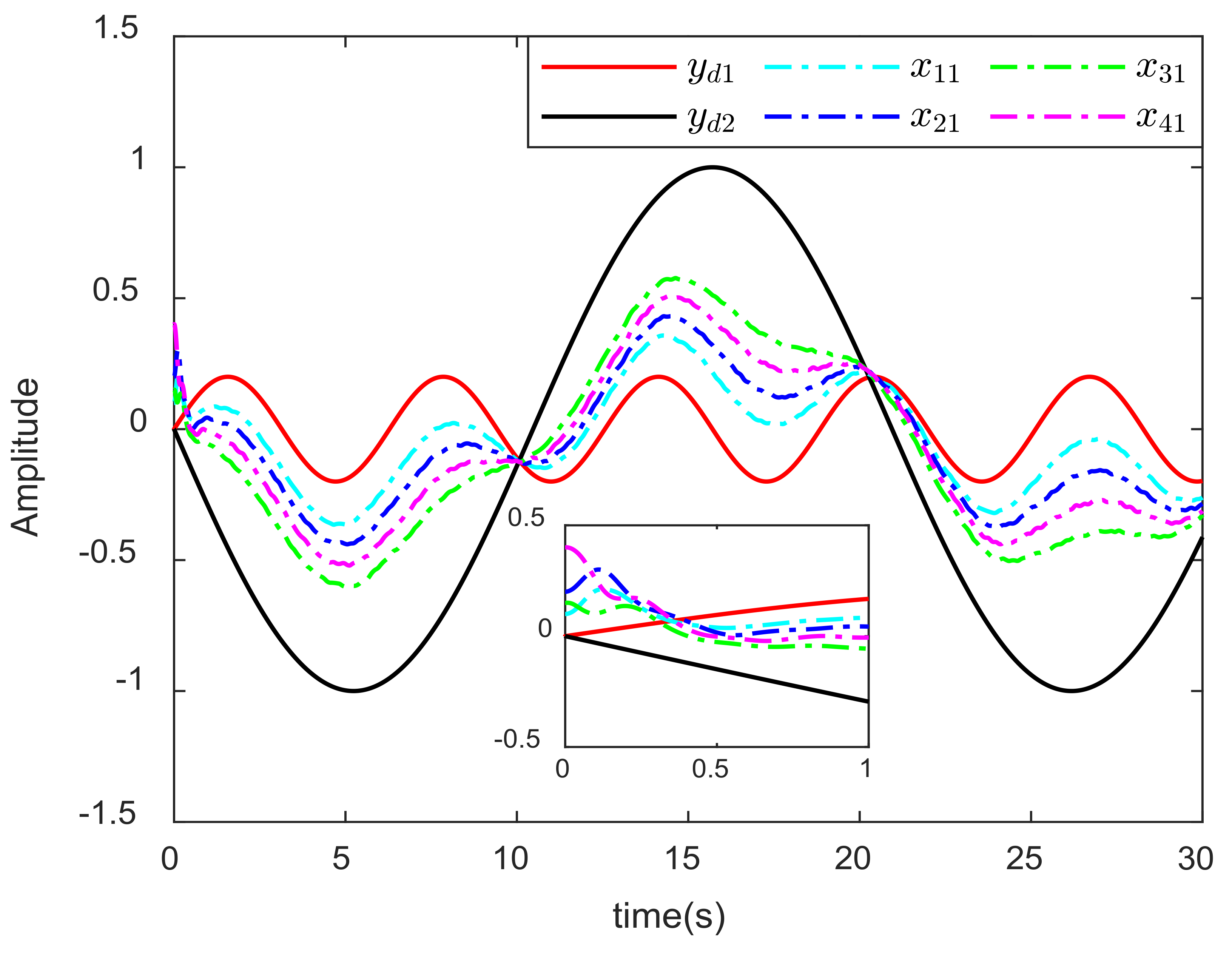
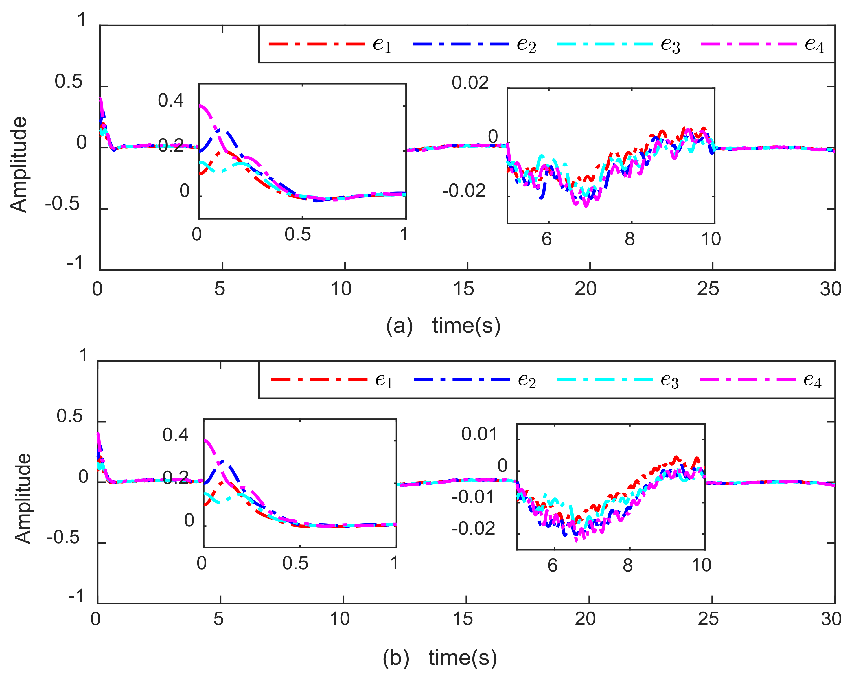
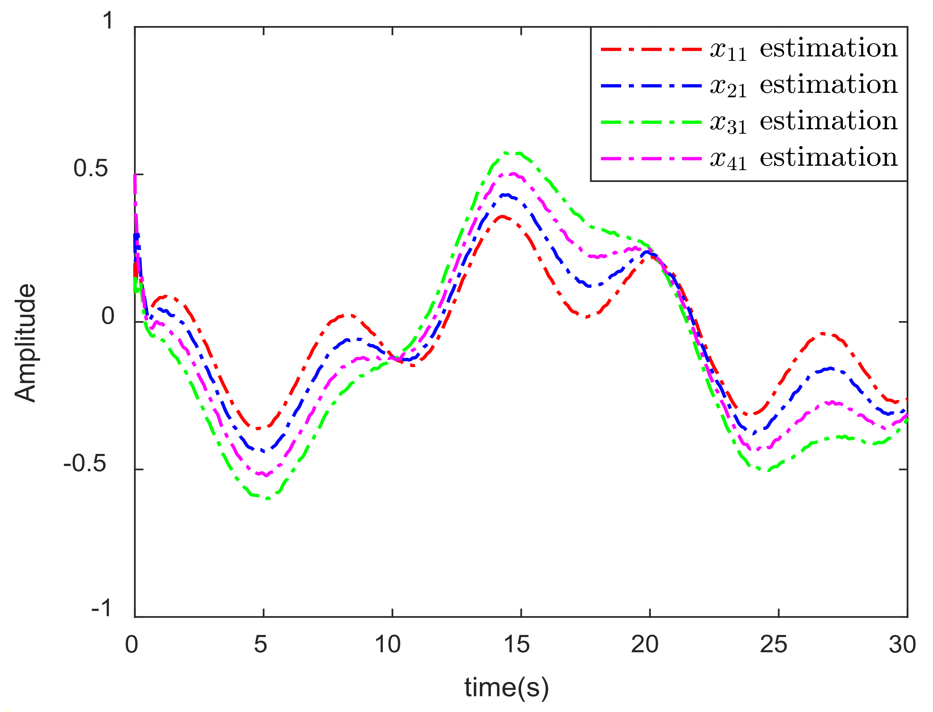
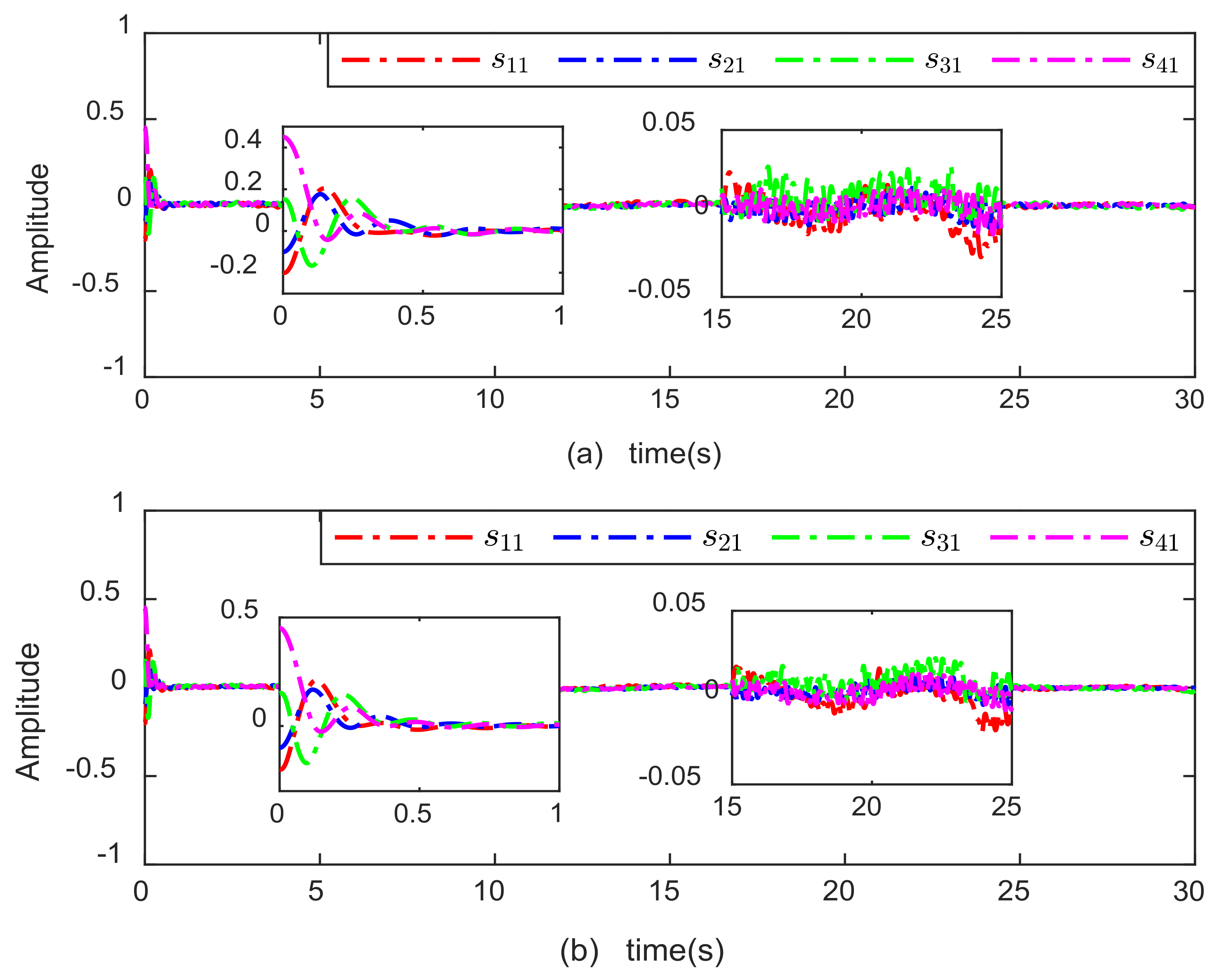
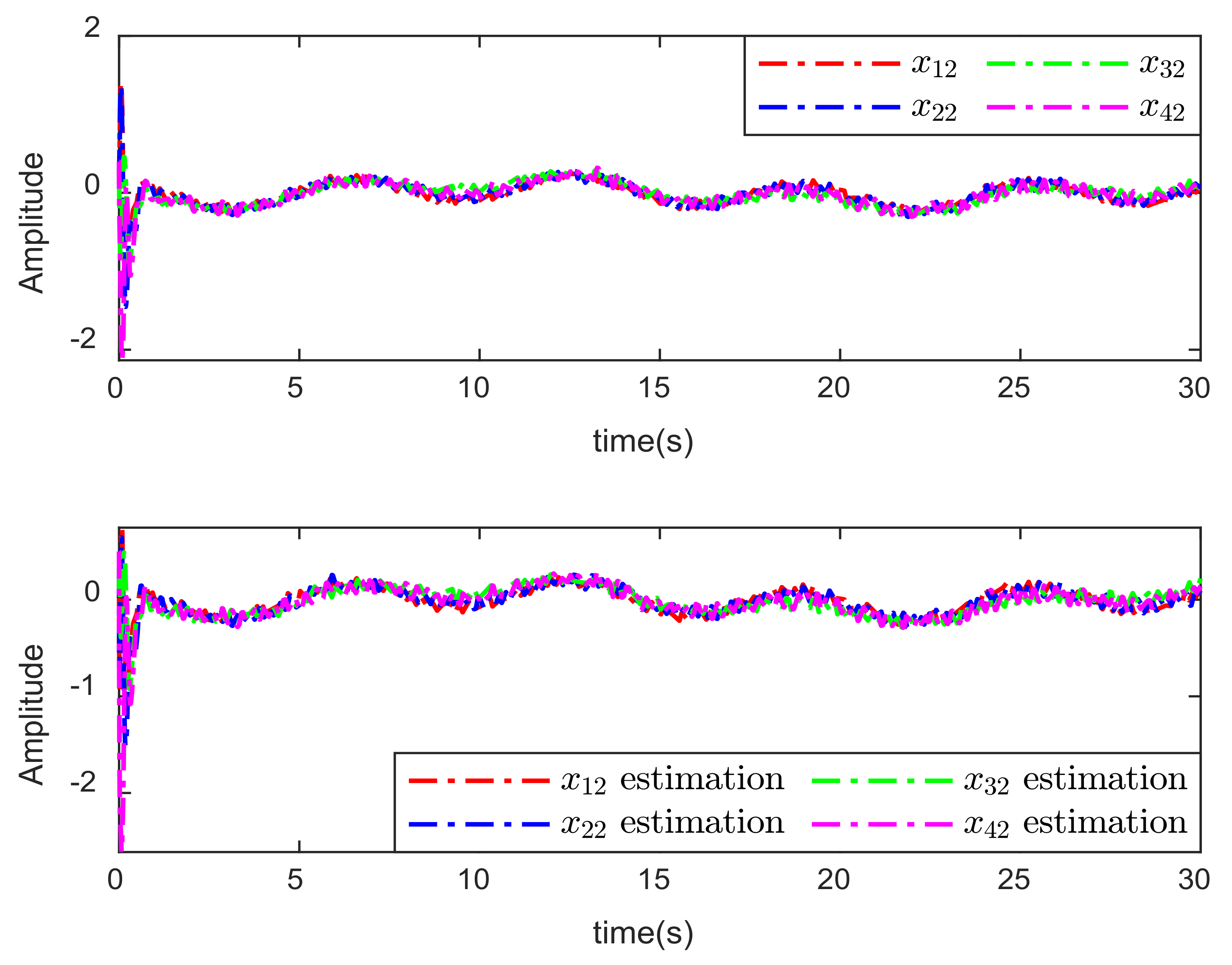
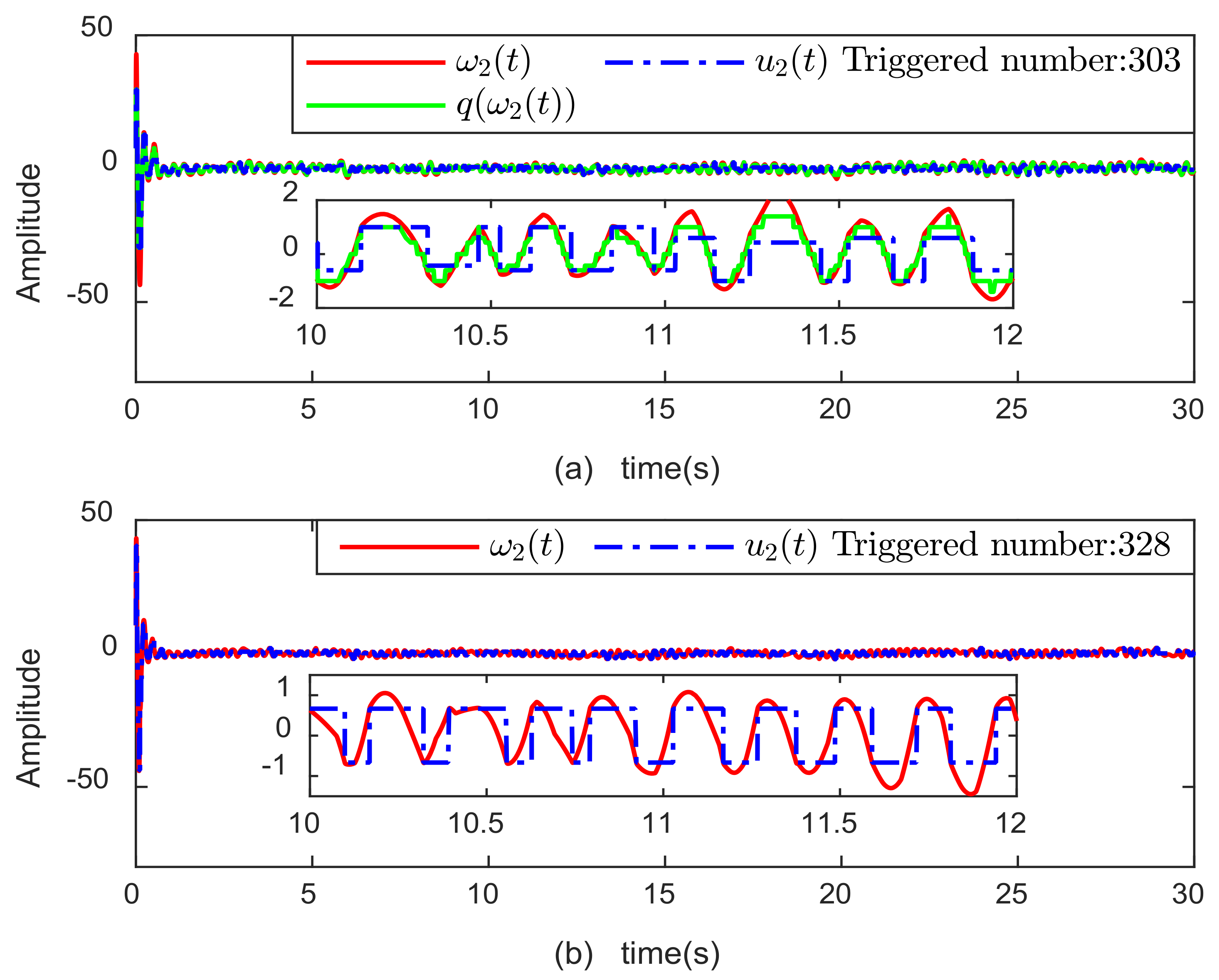
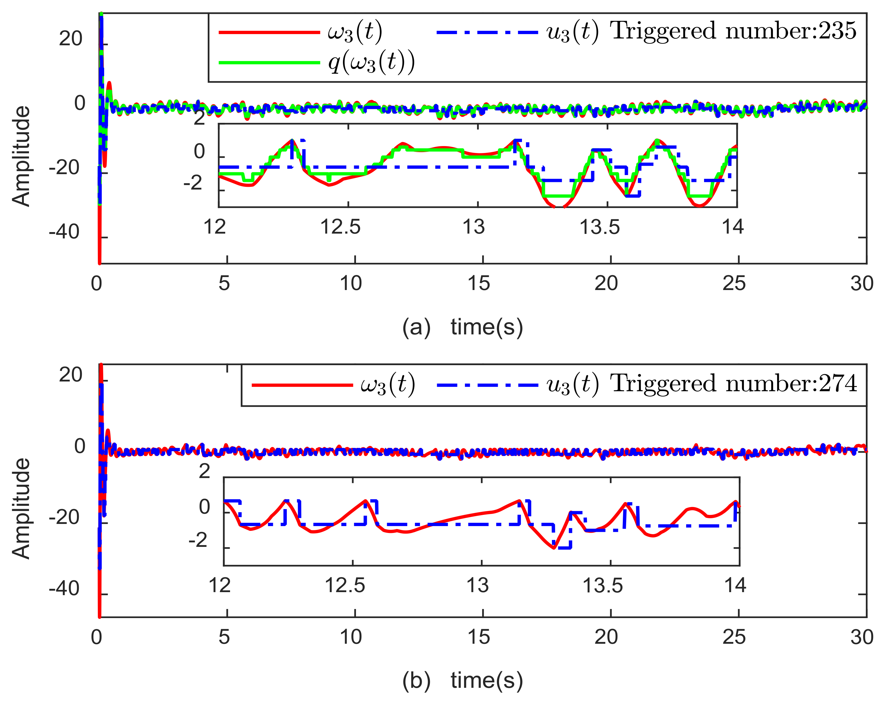
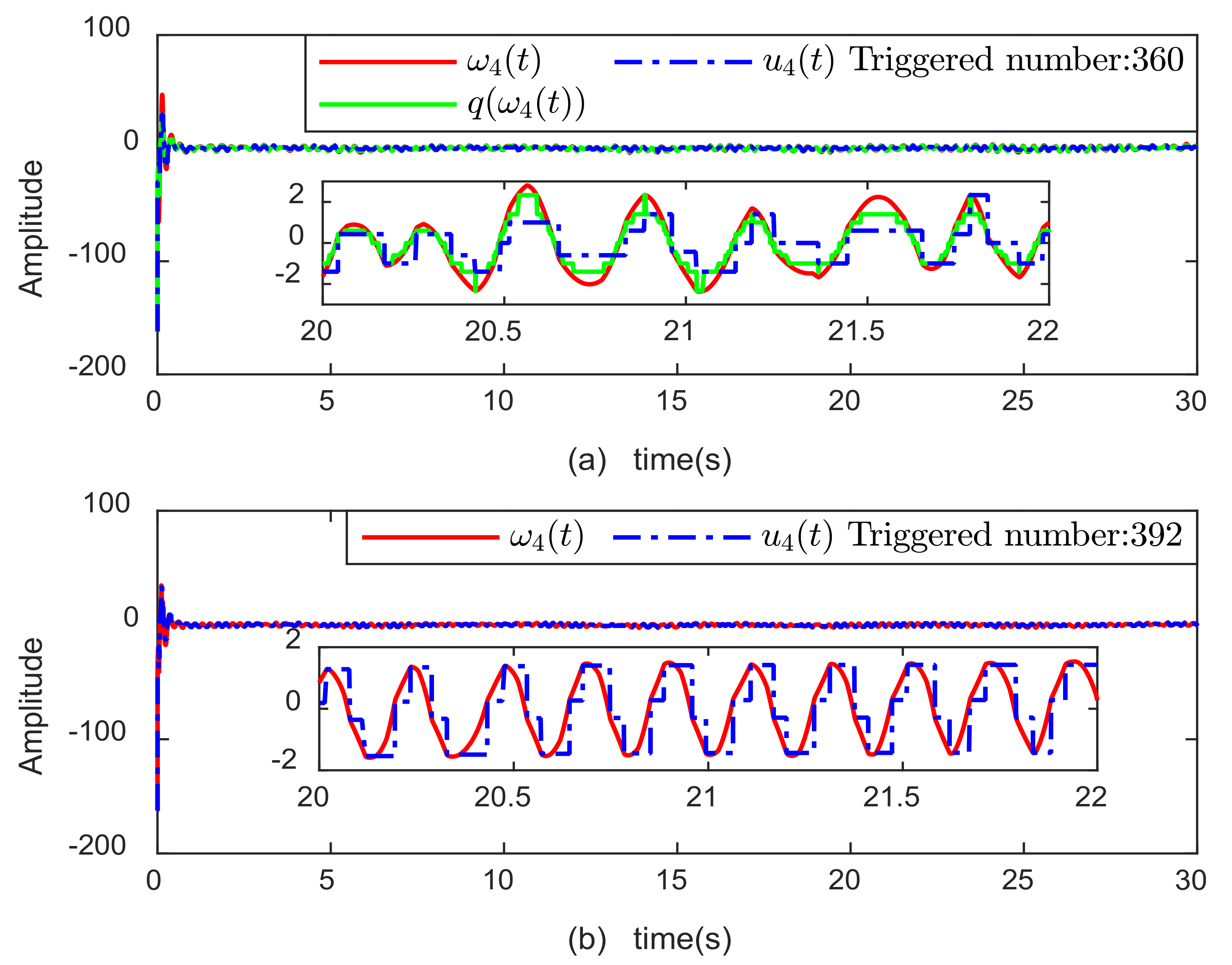
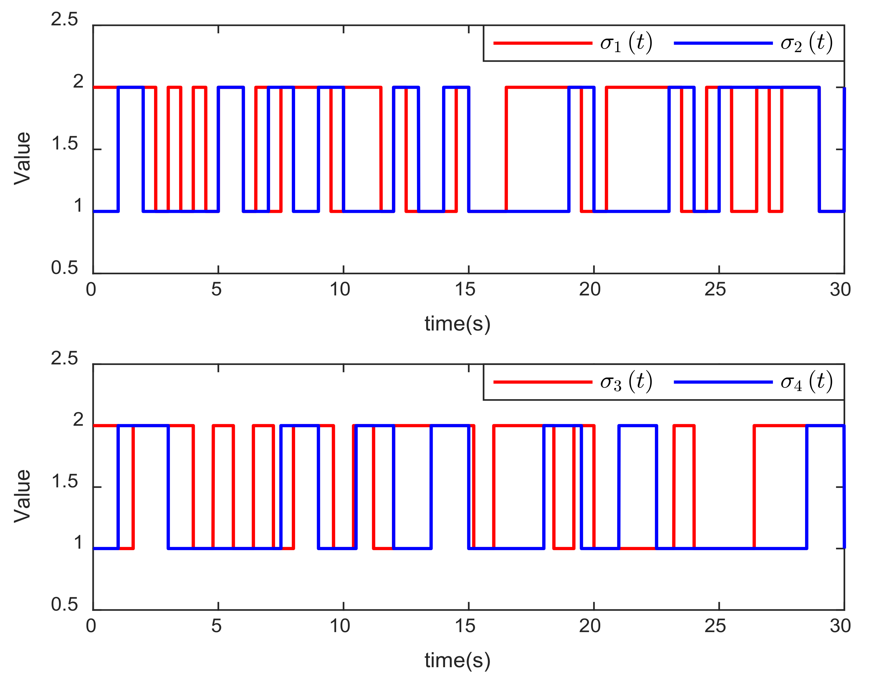
From Equation (87), we have

$$\begin{array}{c}\hfill {\Delta }_i\left(t\right)=q_i\left({\omega }_i\left(t\right)\right)-u_i\left(t\right)={\beta }_{i1}\left(t\right){\kappa }_{i1}{u}_i\left(t\right)+{\beta }_{i2}\left(t\right)H_{i1}\end{array}$$

(88)

where ${\beta }_{i1}\left(t\right)$, ${\beta }_{i2}\left(t\right)$ are time-varying parameters satisfying $\left|{\beta }_{i1}\left(t\right)\right|\le 1$, $\left|{\beta }_{i2}\left(t\right)\right|\le 1$. Accordingly, one can obtain

$$\begin{array}{c}\hfill u_i\left(t\right)=\frac{q_i\left({\omega }_i\left(t\right)\right)-{\beta }_{i2}\left(t\right)H_{i1}}{1+{\beta }_{i1}\left(t\right){\kappa }_{i1}}.\end{array}$$

(89)

Thus, it follows that

$$\begin{array}{cc}\hfill D^{\alpha }{V}_n& \le D^{\alpha }{V}_{n-1}+\sum _{i=1}^N\left\{s_{i,n}^{}\left[\frac{q_i\left({\omega }_i\left(t\right)\right)-{\beta }_{i2}\left(t\right)H_{i1}}{1+{\beta }_{i1}\left(t\right){\kappa }_{i1}}\right.\right.+k_{i,n}{e}_{i,1}+{\tilde{\theta }}_{i,n}^T{\phi }_{i,n}+{\theta }_{i,n}^T{\phi }_{i,n}\hfill \\ \hfill & +{\epsilon }_{i,n}^q+\Delta f_{i,n}^q\left.-D^{\alpha }{v}_{i,n}\right]-\frac{1}{{\sigma }_{i,n}}{\tilde{\theta }}_{i,n}^T{D}^{\alpha }{\theta }_{i,n}-\frac{1}{r_{i,n}}{\tilde{\delta }}_{i,n}^{}{D}^{\alpha }{\delta }_{i,n}^{}\left.+w_{i,n}^{}{D}^{\alpha }{w}_{i,n}^{}\right\}.\hfill \end{array}$$

(90)

Substituting Equations (81) and (82) into (90), we can obtain

$$\begin{array}{cc}\hfill D^{\alpha }{V}_n& \le D^{\alpha }{V}_{n-1}+\sum _{i=1}^N\{s_{i,n}^{}[\frac{q_i\left({\omega }_i\left(t\right)\right)-{\beta }_{i2}\left(t\right)H_{i1}}{1+{\beta }_{i1}\left(t\right){\kappa }_{i1}}+{\theta }_{i,n}^T{\phi }_{i,n}-D^{\alpha }{v}_{i,n}]+s_{i,n}^{}(k_{i,n}{e}_{i,1}+{\tilde{\theta }}_{i,n}^T{\phi }_{i,n}\hfill \\ \hfill & +{\epsilon }_{i,n}^q+\Delta f_{i,n}^q)-\frac{1}{{\sigma }_{i,n}}{\tilde{\theta }}_{i,n}^T\left({\sigma }_{i,n}{\phi }_{i,n}{s}_{i,n}-{\rho }_{i,n}{\theta }_{i,n}\right)-\frac{1}{r_{i,n}}{\tilde{\delta }}_{i,n}^{}\left(r_{i,n}\left|s_{i,n}\right|-{\eta }_{i,n}{\delta }_{i,n}\right)+w_{i,n}^{}{D}^{\alpha }{w}_{i,n}^{}\}.\hfill \end{array}$$

(91)

Then, we can obtain

$$\begin{array}{cc}\hfill D^{\alpha }{V}_n& \le D^{\alpha }{V}_{n-1}+\sum _{i=1}^N\left\{s_{i,n}^{}\left[\frac{q_i\left({\omega }_i\left(t\right)\right)-{\beta }_{i2}\left(t\right)H_{i1}}{1+{\beta }_{i1}\left(t\right){\kappa }_{i1}}+{\overline{\alpha }}_{in}\right]\right.-c_{in}{s}_{i,n}^2-\frac{3}{2}{s}_{i,n}^2\hfill \\ \hfill & -\left|s_{i,n}\right|{\delta }_{i,n}+s_{i,n}^{}\left({\epsilon }_{i,n}^q+\Delta f_{i,n}^q\right)+\frac{{\rho }_{i,n}}{{\sigma }_{i,n}}{\tilde{\theta }}_{i,n}^T{\theta }_{i,n}+s_{i,n}^{}{k}_{i,n}{e}_{i,1}\hfill \\ \hfill & -\frac{1}{r_{i,n}}{\tilde{\delta }}_{i,n}^{}\left(r_{i,n}\left|s_{i,n}\right|\right.\left.\left.-{\eta }_{i,n}{\delta }_{i,n}\right)+w_{i,n}^{}{D}^{\alpha }{w}_{i,n}^{}\right\}.\hfill \end{array}$$

(92)

Similar to the previous calculation, we have

$$\begin{array}{c}\hfill s_{i,n}{k}_{i,n}{e}_{i,1}\le \frac{1}{2}{s}_{i,n}^2+\frac{1}{2}{k}_{i,n}^2{∥e_{i,1}∥}^2\end{array}$$

(93)

$$\begin{array}{c}\hfill s_{i,n}\left({\epsilon }_{i,n}^q+\Delta f_{i,n}^q\right)\le \left|s_{i,n}\right|\left({\tilde{\delta }}_{i,n}+{\delta }_{i,n}\right).\end{array}$$

(94)

From Equations (92)–(94), we can obtain

$$\begin{array}{cc}\hfill D^{\alpha }{V}_n\le D^{\alpha }{V}_{n-1}& +\sum _{i=1}^N\left\{s_{i,n}^{}\left[\frac{q_i\left({\omega }_i\left(t\right)\right)-{\beta }_{i2}\left(t\right)H_{i1}}{1+{\beta }_{i1}\left(t\right){\kappa }_{i1}}+{\overline{\alpha }}_{in}\right]\right.-c_{in}{s}_{i,n}^2-s_{i,n}^2\hfill \\ \hfill & +\frac{{\rho }_{i,n}}{{\sigma }_{i,n}}{\tilde{\theta }}_{i,n}^T{\theta }_{i,n}+\frac{{\eta }_{i,n}}{r_{i,n}}{\tilde{\delta }}_{i,n}^{}{\delta }_{i,n}+\frac{1}{2}{k}_{i,n}^2{∥e_{i,1}∥}^2\left.+w_{i,n}^{}\left(-\frac{w_{i,n}}{{\lambda }_{i,n}}+B_{i,n}\right)\right\}.\hfill \end{array}$$

(95)

By employing Young’s inequality, we have

$$\begin{array}{c}\hfill w_{i,n}{B}_{i,n}\le \frac{1}{2}{w}_{i,n}^2+\frac{1}{2}{M}_{i,n}^2.\end{array}$$

(96)

Then we have

$$\begin{array}{cc}\hfill D^{\alpha }{V}_n\le D^{\alpha }{V}_{n-1}& +\sum _{i=1}^N\left\{s_{i,n}^{}\left[\frac{q_i\left({\omega }_i\left(t\right)\right)-{\beta }_{i2}\left(t\right)H_{i1}}{1+{\beta }_{i1}\left(t\right){\kappa }_{i1}}+{\overline{\alpha }}_{in}\right]\right.-c_{in}{s}_{i,n}^2-s_{i,n}^2\hfill \\ \hfill & +\frac{{\rho }_{i,n}}{{\sigma }_{i,n}}{\tilde{\theta }}_{i,n}^T{\theta }_{i,n}+\frac{{\eta }_{i,n}}{r_{i,n}}{\tilde{\delta }}_{i,n}^{}{\delta }_{i,n}+\frac{1}{2}{k}_{i,n}^2{∥e_{i,1}∥}^2\left.-\frac{w_{i,n}^2}{{\lambda }_{i,n}}+\frac{1}{2}{w}_{i,n}^2+\frac{1}{2}{M}_{i,n}^2\right\}.\hfill \end{array}$$

(97)

Substituting Equations (5), (84) and (85) into (97), we have

$$\begin{array}{cc}\hfill D^{\alpha }{V}_n\le D^{\alpha }{V}_{n-1}& +\sum _{i=1}^N\left\{-c_{in}{s}_{i,n}^2-s_{i,n}^2+\frac{{\rho }_{i,n}}{{\sigma }_{i,n}}{\tilde{\theta }}_{i,n}^T{\theta }_{i,n}\right.+\frac{{\eta }_{i,n}}{r_{i,n}}{\tilde{\delta }}_{i,n}^{}{\delta }_{i,n}+\frac{1}{2}{k}_{i,n}^2{∥e_{i,1}∥}^2-\frac{w_{i,n}^2}{{\lambda }_{i,n}}\hfill \\ \hfill & \left.+\frac{1}{2}{w}_{i,n}^2+\frac{1}{2}{s}_{i,n}^2+\frac{{\omega }_{min}^2}{2{\left(1-{\kappa }_{i1}\right)}^2}+\frac{1}{2}{M}_{i,n}^2+\frac{2{\kappa }_{i2}}{1-{\kappa }_{i1}}\right\}.\hfill \end{array}$$

(98)

From Equation (71), we can obtain

$$\begin{array}{cc}\hfill D^{\alpha }{V}_{n-1}& \le -q_{n-1}{∥e∥}^2+\frac{1}{2}{∥P\epsilon ∥}^2+\sum _{i=1}^N\sum _{l=1}^n\frac{1}{2}{\tilde{\theta }}_{i,l}^T{\tilde{\theta }}_{i,l}\hfill \\ \hfill & +\sum _{i=1}^N\left\{\sum _{l=1}^{n-1}\left(-c_{i,,l}{s}_{i,l}^2+\frac{{\rho }_{i,l}}{{\sigma }_{i,l}}{\tilde{\theta }}_{i,l}^T{\theta }_{i,l}+\frac{{\eta }_{i,l}}{r_{i,l}}{\tilde{\delta }}_{i,l}{\delta }_{i,l}\right)\right.\hfill \\ \hfill & +\sum _{j=1}^N{a}_{ij}\left(\frac{{\rho }_{j,1}}{{\sigma }_{j,1}}{\tilde{\theta }}_{j,1}^T{\theta }_{j,1}+\frac{{\eta }_{j,1}}{r_{j,1}}{\tilde{\delta }}_{j,1}{\delta }_{j,1}\right)-\left(\frac{1}{{\lambda }_{i,2}}-\frac{1}{2}-\frac{d_i^2}{2}\right)w_{i,2}^2\hfill \\ \hfill & -\sum _{l=3}^{n-1}\left(\frac{1}{{\lambda }_{i,l}}-1\right)w_{i,l}^2+\frac{1}{2}\left(s_{i,n}^2+w_{i,n}^2\right)\left.+\sum _{l=2}^{n-1}\frac{1}{2}{M}_{i,l}^2\right\}.\hfill \end{array}$$

(99)

Substituting (99) into (98) yields

$$\begin{array}{cc}\hfill D^{\alpha }{V}_n& \le -q_n{∥e∥}^2+\frac{1}{2}{∥P\epsilon ∥}^2+\sum _{i=1}^N\sum _{l=1}^n\frac{1}{2}{\tilde{\theta }}_{i,l}^T{\tilde{\theta }}_{i,l}+\sum _{i=1}^N\left\{\sum _{l=1}^n\left(-c_{i,,l}{s}_{i,l}^2+\frac{{\rho }_{i,l}}{{\sigma }_{i,l}}{\tilde{\theta }}_{i,l}^T{\theta }_{i,l}+\frac{{\eta }_{i,l}}{r_{i,l}}{\tilde{\delta }}_{i,l}{\delta }_{i,l}\right)\right.\hfill \\ \hfill & +\sum _{j=1}^N{a}_{ij}\left(\frac{{\rho }_{j,1}}{{\sigma }_{j,1}}{\tilde{\theta }}_{j,1}^T{\theta }_{j,1}+\frac{{\eta }_{j,1}}{r_{j,1}}{\tilde{\delta }}_{j,1}{\delta }_{j,1}\right)-\left(\frac{1}{{\lambda }_{i,2}}-\frac{1}{2}-\frac{d_i^2}{2}\right)w_{i,2}^2\hfill \\ \hfill & -\sum _{l=3}^n\left(\frac{1}{{\lambda }_{i,l}}-1\right)w_{i,l}^2\left.+\frac{{\omega }_{min}^2}{2{\left(1-{\kappa }_{i1}\right)}^2}+\sum _{l=2}^n\frac{1}{2}{M}_{i,l}^2+\frac{2{\kappa }_{i2}}{1-{\kappa }_{i1}}\right\}\hfill \end{array}$$

(100)

where $q_n=q_{n-1}-{\sum }_{i=1}^N{k}_{i,n}^2$. According to Lemma 4, we have

$${\tilde{\theta }}_{*,l}^T{\theta }_{*,l}\le -\frac{1}{2}{\tilde{\theta }}_{*,l}^T{\tilde{\theta }}_{*,l}+\frac{1}{2}{\theta }_{*,l}^{*T}{\theta }_{*,l}^{*}$$

(101)

$${\tilde{\delta }}_{*,l}{\delta }_{*,l}\le -\frac{1}{2}{{\tilde{\delta }}_{*,l}}^2+\frac{1}{2}{{\delta }_{*,l}}^{*2}.$$

(102)

From Equations (100)–(102), we can obtain

$$\begin{array}{cc}\hfill D^{\alpha }{V}_n& \le -q_n{∥e∥}^2+\frac{1}{2}{∥P\epsilon ∥}^2+\sum _{i=1}^N\sum _{l=1}^n\frac{1}{2}{\tilde{\theta }}_{i,l}^T{\tilde{\theta }}_{i,l}\hfill \\ \hfill & +\sum _{i=1}^N\left\{\sum _{l=1}^n\left(-c_{i,,l}{s}_{i,l}^2-\frac{{\rho }_{i,l}}{2{\sigma }_{i,l}}{\tilde{\theta }}_{i,l}^T{\tilde{\theta }}_{i,l}-\frac{{\eta }_{i,l}}{2r_{i,l}}{\tilde{\delta }}_{i,l}^2\right)\right.+\sum _{j=1}^N{a}_{ij}\left(-\frac{{\rho }_{j,1}}{2{\sigma }_{j,1}}{\tilde{\theta }}_{j,1}^T{\tilde{\theta }}_{j,1}-\frac{{\eta }_{j,1}}{2r_{j,1}}{\tilde{\delta }}_{j,1}^2\right)\hfill \\ \hfill & -\left(\frac{1}{{\lambda }_{i,2}}-\frac{1}{2}-\frac{d_i^2}{2}\right)w_{i,2}^2-\sum _{l=3}^n\left(\frac{1}{{\lambda }_{i,l}}-1\right)w_{i,l}^2\hfill \\ \hfill & +\sum _{l=1}^n\left(\frac{{\rho }_{i,l}}{2{\sigma }_{i,l}}{\theta }_{i,l}^{*T}{\theta }_{i,l}^{*}+\frac{{\eta }_{i,l}}{2r_{i,l}}{\delta }_{i,l}^{*2}\right)+\sum _{j\in N_i}{a}_{ij}\left(\frac{{\rho }_{j,1}}{2{\sigma }_{j,1}}{\theta }_{j,1}^{*T}{\theta }_{j,1}^{*}+\frac{{\eta }_{j,1}}{2r_{j,1}}{\delta }_{j,1}^{*2}\right)\hfill \\ \hfill & \left.+\frac{{\omega }_{min}^2}{2{\left(1-{\kappa }_{i1}\right)}^2}+\sum _{l=2}^n\frac{1}{2}{M}_{i,l}^2+\frac{2{\kappa }_{i2}}{1-{\kappa }_{i1}}\right\}.\hfill \end{array}$$

(103)

Denote

$$\begin{array}{cc}\hfill \xi & =\frac{1}{2}{∥P\epsilon ∥}^2+\sum _{i=1}^N\left\{\sum _{l=1}^n\left(\frac{{\rho }_{i,l}}{2{\sigma }_{i,l}}{\theta }_{i,l}^{*T}{\theta }_{i,l}^{*}+\frac{{\eta }_{i,l}}{2r_{i,l}}{\delta }_{i,l}^{*2}\right)\right.+\sum _{j=1}^N{a}_{ij}\left(\frac{{\rho }_{j,1}}{2{\sigma }_{j,1}}{\theta }_{j,1}^{*T}{\theta }_{j,1}^{*}+\frac{{\eta }_{j,1}}{2r_{j,1}}{\delta }_{j,1}^{*2}\right)\hfill \\ \hfill & \left.+\frac{{\omega }_{min}^2}{2{\left(1-{\kappa }_{i1}\right)}^2}+\sum _{l=2}^n\frac{1}{2}{M}_{i,l}^2+\frac{2{\kappa }_{i2}}{1-{\kappa }_{i1}}\right\}.\hfill \end{array}$$

(104)

Then Equation (103) can be written as

$$\begin{array}{cc}\hfill D^{\alpha }{V}_n& \le -q_n{∥e∥}^2+\sum _{i=1}^N\left\{\sum _{l=1}^n\left(-c_{i,,l}{s}_{i,l}^2-\left(\frac{{\rho }_{i,l}}{2{\sigma }_{i,l}}-\frac{1}{2}\right){\tilde{\theta }}_{i,l}^T{\tilde{\theta }}_{i,l}\right.\right.\hfill \\ \hfill & \left.-\frac{{\eta }_{i,l}}{2r_{i,l}}{\tilde{\delta }}_{i,l}^2\right)+\sum _{j=1}^N{a}_{ij}\left(-\frac{{\rho }_{j,1}}{2{\sigma }_{j,1}}{\tilde{\theta }}_{j,1}^T{\tilde{\theta }}_{j,1}-\frac{{\eta }_{j,1}}{2r_{j,1}}{\tilde{\delta }}_{j,1}^2\right)\hfill \\ \hfill & -\left(\frac{1}{{\lambda }_{i,2}}-\frac{1}{2}-\frac{d_i^2}{2}\right)w_{i,2}^2-\left.\sum _{l=3}^n\left(\frac{1}{{\lambda }_{i,l}}-1\right)w_{i,l}^2\right\}+\xi \hfill \end{array}$$

(105)

where $c_{i,l}>0,\left(l=1,\dots n\right)$, $\left(\frac{1}{{\lambda }_{i,2}}-\frac{1}{2}-\frac{d_i^2}{2}\right)>0$, $\left(\frac{1}{{\lambda }_{i,l}}-1\right)>0,l=3,\dots ,n$, $\left(\frac{{\rho }_{i,l}}{2{\sigma }_{i,l}}-\frac{1}{{\tau }_i}\right)>0$, $\frac{{\eta }_{i,l}}{2r_{i,l}}>0$, $\frac{{\rho }_{i,l}}{2{\sigma }_{i,l}}>0$.

Define

$$\begin{array}{c}\hfill C=min\left\{2q_n/\phantom{2q_n{\lambda }_{min}\left(P\right)}{\lambda }_{min}\left(P\right),2c_{i,l},2\left(\frac{{\rho }_{i,l}}{2{\sigma }_{i,l}}-\frac{1}{2}\right),\frac{{\eta }_{i,l}}{r_{i,l}},\frac{{\rho }_{i,l}}{{\sigma }_{i,l}},\right.\left.2\left(\frac{1}{{\lambda }_{i,2}}-\frac{1}{2}-\frac{{d_i}^2}{2}\right),2\left(\frac{1}{{\lambda }_{i,l}}-1\right)\right\}.\end{array}$$

(106)

Then Equation (105) becomes

$$D^{\alpha }{V}_n\le -C{V}_n+\xi .$$

(107)

According to Equation (107), we can obtain

$$D^{\alpha }{V}_n+Q\left(t\right)=-C{V}_n+\xi$$

(108)

where $Q\left(t\right)\ge 0$.

According to Lemma 6, we can obtain

$$\begin{array}{c}{V}_n\le V\left(0\right)E_{\alpha }\left(-C{t}^{\alpha }\right)+\frac{\xi \mu }{C}.\end{array}$$

(109)

Then, we have

$$\underset{t\to \infty }{lim}\left|V_n\left(t\right)\right|\le \frac{\xi \mu }{C}.$$

(110)

Since $\frac{1}{2}{\left|s_{i,1}\right|}^2\le V_n\left(t\right)$, and we can obtain $\left|\left|s_{i,1}\right|\right|\le \sqrt{\frac{2\xi \mu }{C}}$, invoking $s_{i,1}={\sum }_{j=1}^N{a}_{ij}\left(y_i-y_j\right)$$+{\sum }_{j=N+1}^{N+M}{a}_{ij}\left(y_i-y_{dj}\left(t\right)\right)$, note the fact that $s_1=L_{1}y+L_{2}r\left(t\right)$, where $s_1={\left[s_{1,1},\dots ,s_{N,1}\right]}^T$. Because the convex hull spanned by leaders is defined as $r_d\left(t\right)=-L_1^{-1}{L}_{2}r\left(t\right)$, then, the containment errors satisfy $∥e∥=∥y-r_d\left(t\right)∥\le \frac{\sqrt{2\xi \mu /\phantom{2\xi \mu C}C}}{{∥L_1∥}_F}$.

The proof process that the proposed control method can avoid Zeno phenomenon is as follows:

By ${\Delta }_i\left(t\right)=q_i\left({\omega }_i\left(t\right)\right)-u_i\left(t\right)$, we have $D^{\alpha }\left|{\Delta }_i\right|=D^{\alpha }\left(\sqrt{{\Delta }_i·{\Delta }_i}\right)=sign\left({\Delta }_i\right)D^{\alpha }\left({\Delta }_i\right)$ $\le \left|D^{\alpha }\left(q_i\left({\omega }_i\left(t\right)\right)\right)\right|=\left|D^{\alpha }\left(H\left({\omega }_i\right){\omega }_i\left(t\right)\right)\right|\le \left(1+d\right)\left|D^{\alpha }\left({\omega }_i\left(t\right)\right)\right|$. According to Equation (84), $D^{\alpha }\left({\omega }_i\left(t\right)\right)$ is bounded in a closed interval $[0,t]$. Therefore, there exists a constant $\varsigma >0$ such that $\left|D^{\alpha }\left({\omega }_i\left(t\right)\right)\right|\le \varsigma$. From $\Delta \left(t_k\right)=0$ and ${lim}_{t\to t_{k+1}}\Delta \left(t\right)=H_{i1}$, thus, there exists $t^{*}$ such that $t^{*}\ge H_{i1}/\phantom{H_{i1}\varsigma }\varsigma$. Therefore, there exists $t^{*}\ge 0$ such that $\forall k\in z^{+}$, $\left\{t_{k+1}-t_k\right\}\ge t^{*}$, the Zeno phenomenon will not occur.

Remark 1.

It should be noted that the classical local theories used in this paper do not have the ability to describe the material heterogeneities and the fluctuations of different scales. In future research, we will use a more appropriate definition of a fractional differential, such as the Atangana-Baleanu [50] or Caputo-Fabrizio [51] fractional derivative definition.

4. Simulation

In this section, to verify the effectiveness of the proposed method, the following fractional Duffing-Holmes chaotic system [52] is considered.

$$\left\{\begin{array}{cc}\hfill D^{\alpha }{x}_{i,1}& =x_{i,2}+f_{i,1}^q\left(X_{i,1}\right)\hfill \\ \hfill D^{\alpha }{x}_{i,2}& =u_i\left(t\right)+f_{i,2}^q\left(X_{i,2}\right)\hfill \\ \hfill y_i& =x_{i,1}\hfill \end{array}\right.$$

(111)

where the system order is $\alpha =0.98$, $i=1,2,3,4$. ${y_d}_1=0.2sint$ and ${y_d}_2=sin0.3t$ are defined as the leaders. The unknown functions are $f_{1,1}^q=f_{2,1}^q=f_{3,1}^q=f_{4,1}^q=0$, $f_{1,2}^1=x_{1,1}-0.25x_{1,2}-x_{1,1}^3+0.3cos\left(t\right),f_{1,2}^2=2x_{1,1}-0.25x_{1,2}-x_{1,1}^3,f_{2,2}^1=x_{2,1}-0.25x_{2,2}-x_{2,1}^3+0.1(x_{2,1}^2+x_{2,2}^2{)}^{1/2}$, $f_{2,2}^2=x_{2,1}^2,f_{3,2}^1=x_{3,1}-0.25x_{3,2}-x_{3,1}^3+0.2sin\left(t\right)(x_{3,1}^2+2x_{3,2}^2{)}^{1/2}$, $f_{3,2}^2=x_{3,1}^2-x_{3,1}^3,f_{4,2}^1=x_{4,1}^2$, and $f_{4,2}^2=x_{4,1}-0.25x_{4,2}-x_{4,1}^3+0.2sin\left(t\right)(2x_{4,1}^2+2x_{4,2}^2{)}^{1/2}.$ We chose the design parameters as $c_{i,1}=20$, $c_{i,2}=30$, ${\sigma }_{i,2}=r_{i,2}=1$, ${\rho }_{i,2}=40$, ${\eta }_{i,2}=20$, ${\lambda }_{i,2}=0.05$, ${\kappa }_{i1}=0.5$, ${\kappa }_{i2}=2$, $M_{i,1}=1$, ${\omega }_{min}=1$, and $d=0.4$. We chose the initial conditions of the system as $x_1\left(0\right)={\left[0.1,0.1\right]}^T$, $x_2\left(0\right)={\left[0.2,0.2\right]}^T$, $x_3\left(0\right)={\left[0.3,0.3\right]}^T$, and $x_4\left(0\right)={\left[0.4,0.4\right]}^T$. The observer initial conditions were chosen as ${\widehat{x}}_1\left(0\right)={\left[0.2,0.2\right]}^T$, ${\widehat{x}}_2\left(0\right)={\left[0.3,0.3\right]}^T$, ${\widehat{x}}_3\left(0\right)={\left[0.4,0.4\right]}^T$, and ${\widehat{x}}_4\left(0\right)={\left[0.5,0.5\right]}^T$.

The communication graph of the multiagent system is shown in Figure 1. Figure 2, Figure 3, Figure 4, Figure 5, Figure 6, Figure 7, Figure 8, Figure 9, Figure 10, Figure 11, Figure 12 and Figure 13 show the simulation results. Figure 2 displays the trajectories of ${y_d}_1$, ${y_d}_2$ and $x_{i,1}\left(i=1,\cdots ,4\right)$. Figure 3 shows the trajectories of the containment tracking errors. Figure 3a shows the trajectories of the containment tracking errors based on the event-triggered quantized controller, and Figure 3b shows the trajectories of containment tracking errors based on the event-triggered controller without input quantization. Figure 4 shows the trajectories of the $x_{i,1}\left(i=1,\cdots ,4\right)$ estimation values. Figure 5 gives the error surfaces $s_{i,1}$ of the two controllers. Figure 6 gives the trajectories of $x_{i,2}$ and ${\widehat{x}}_{i,2}$. We use $x_{1,1}$ and $x_{1,2}$ as examples in Figure 7 to show the results of the neural network observer designed in this paper. Figure 8, Figure 9, Figure 10 and Figure 11 show the trajectories of ${\omega }_i$, $q\left({\omega }_i\right)$, and $u_i$. Meanwhile, we compared the event-triggered control input without quantitative control technology with the control input mentioned in this article. From Figure 8, Figure 9, Figure 10 and Figure 11, the triggered number of control input via the quanzited mechanism was reduced by 7% to 20%, among which $u_1$ was reduced by 20% (see Figure 8), and $u_4$ was reduced by 7% (see Figure 11). In order to better highlight the advantages of the method proposed in this paper, we have compared the triggered number under different sampling mechanisms. It can be seen from Figure 13 that the proposed method can significantly reduce the number of control input samples. This means that the combination of event-triggered control and quantized control mechanisms can effectively reduce the number of transmissions of control input signals, so it has more practical significance and potential engineering value. Figure 12 shows the trajectories of the switching signal ${\sigma }_i\left(t\right)$. From the simulation results, the proposed method can ensure all followers converge to the leaders’ convex hull, and the control performance is satisfactory.

5. Conclusions

This paper proposed an event-triggered adaptive neural network dynamic surface quantized controller for the switched fractional order multiagent systems containment control problem. The followers considered were fractional order systems and contained arbitrarily switched nonlinear functions and unmeasured states. The hysteresis quantizer that we used can effectively avoid the chattering phenomena. An event-triggered scheme without Zeno behavior was considered, which reduced the utilization of communication resources. An RBF neural network was used to approximate unknown nonlinear functions and construct state observers to obtain unmeasurable states. Fractional derivatives of virtual control laws were obtained by fractional order DSC techniques, while avoiding “explosion of complexity”. Example and simulation results showed that the proposed controller can not only ensure that all followers can converge to the leader’s convex hull but also reduce the sampling frequency of the control input compared with the traditional event-triggered mechanism. With the consideration of dynamic uncertainties and the reduction in communication resources, the control algorithm in this study has a significant practical value, especially in the aspect of network control. Based on the previous work, this paper extended the adaptive dynamic surface control technology to the switched fractional order multiagent system and further studied the bipartite containment control problem under an event-triggered mechanism and control input quantization. Future research will apply this control scheme to real physical systems, such as wing vibration control of fixed-wing aircraft, robot formation control, etc.

References

1. Sun, F.; Lei, C.; Kurths, J. Consensus of heterogeneous discrete-time multi-agent systems with noise over Markov switching topologies. Int. J. Robust Nonlinear Control 2021, 31, 1530–1541. [Google Scholar] [CrossRef]
2. Ma, L.; Wang, Z.; Lam, H.K. Event-triggered mean-square consensus control for time-varying stochastic multi-agent system with sensor saturations. IEEE Trans. Autom. Control 2016, 62, 3524–3531. [Google Scholar] [CrossRef] [Green Version]
3. Mao, J.; Yan, T.; Huang, S.; Li, S.; Jiao, J.g. Sampled-data output feedback leader-following consensus for a class of nonlinear multi-agent systems with input unmodeled dynamics. Int. J. Robust Nonlinear Control 2021, 31, 4203–4226. [Google Scholar] [CrossRef]
4. Deng, F.; Guo, S.; Zhou, R.; Chen, J. Sensor multifault diagnosis with improved support vector machines. IEEE Trans. Autom. Sci. Eng. 2015, 14, 1053–1063. [Google Scholar] [CrossRef]
5. Yao, D.; Dou, C.; Yue, D.; Zhao, N.; Zhang, T. Adaptive neural network consensus tracking control for uncertain multi-agent systems with predefined accuracy. Nonlinear Dyn. 2020, 101, 2249–2262. [Google Scholar] [CrossRef]
6. Guo, X.; Liang, H.; Pan, Y. Observer-Based Adaptive Fuzzy Tracking Control for Stochastic Nonlinear Multi-Agent Systems with Dead-Zone Input. Appl. Math. Comput. 2020, 379, 125269. [Google Scholar] [CrossRef]
7. Tian, Y.; Xia, Q.; Chai, Y.; Chen, L.; Lopes, A.M.; Chen, Y. Guaranteed Cost Leaderless Consensus Protocol Design for Fractional-Order Uncertain Multi-Agent Systems with State and Input Delays. Fractal Fract. 2021, 5, 141. [Google Scholar] [CrossRef]
8. Chen, T.; Yuan, J.; Yang, H. Event-triggered adaptive neural network backstepping sliding mode control of fractional-order multi-agent systems with input delay. J. Vib. Control 2021. [Google Scholar] [CrossRef]
9. Yang, Y.; Liu, F.; Yang, H.; Li, Y.; Liu, Y. Distributed Finite-Time Integral Sliding-Mode Control for Multi-Agent Systems with Multiple Disturbances Based on Nonlinear Disturbance Observers. J. Syst. Sci. Complex. 2021, 34, 995–1013. [Google Scholar] [CrossRef]
10. Shahvali, M.; Azarbahram, A.; Naghibi-Sistani, M.B.; Askari, J. Bipartite consensus control for fractional-order nonlinear multi-agent systems: An output constraint approach. Neurocomputing 2020, 397, 212–223. [Google Scholar] [CrossRef]
11. González, A.; Aragüés, R.; López-Nicolás, G.; Sagüés, C. Weighted predictor-feedback formation control in local frames under time-varying delays and switching topology. Int. J. Robust Nonlinear Control 2020, 30, 3484–3500. [Google Scholar] [CrossRef]
12. Cui, G.; Xu, S.; Chen, X.; Lewis, F.L.; Zhang, B. Distributed containment control for nonlinear multiagent systems in pure-feedback form. Int. J. Robust Nonlinear Control 2018, 28, 2742–2758. [Google Scholar] [CrossRef]
13. Deng, X.; Cui, Y. Adaptive fuzzy containment control for nonlinear multi-agent systems with input delay. Int. J. Syst. Sci. 2021, 52, 1633–1645. [Google Scholar] [CrossRef]
14. Cui, Y.; Liu, X.; Deng, X.; Wang, L. Adaptive Containment Control for Nonlinear Strict-Feedback Multi-Agent Systems with Dynamic Leaders. Int. J. Control 2020, 1–20. [Google Scholar] [CrossRef]
15. Li, Y.; Hua, C.; Wu, S.; Guan, X. Output feedback distributed containment control for high-order nonlinear multiagent systems. IEEE Trans. Cybern. 2017, 47, 2032–2043. [Google Scholar] [CrossRef]
16. Parsa, M.; Danesh, M. Containment control of high-order multi-agent systems with heterogeneous uncertainties, dynamic leaders, and time delay. Asian J. Control 2021, 23, 799–810. [Google Scholar] [CrossRef]
17. Pan, H.; Yu, X.; Yang, G.; Xue, L. Robust consensus of fractional-order singular uncertain multi-agent systems. Asian J. Control 2020, 22, 2377–2387. [Google Scholar] [CrossRef]
18. Lü, H.; He, W.; Han, Q.L.; Ge, X.; Peng, C. Finite-time containment control for nonlinear multi-agent systems with external disturbances. Inf. Sci. 2020, 512, 338–351. [Google Scholar] [CrossRef]
19. Xu, C.; Liao, M.; Li, P.; Yao, L.; Qin, Q.; Shang, Y. Chaos Control for a Fractional-Order Jerk System via Time Delay Feedback Controller and Mixed Controller. Fractal Fract. 2021, 5, 257. [Google Scholar] [CrossRef]
20. Jahanzaib, L.S.; Trikha, P.; Matoog, R.T.; Muhammad, S.; Al-Ghamdi, A.; Higazy, M. Dual Penta-Compound Combination Anti-Synchronization with Analysis and Application to a Novel Fractional Chaotic System. Fractal Fract. 2021, 5, 264. [Google Scholar] [CrossRef]
21. İlknur, K.; AKÇETİN, E.; Yaprakdal, P. Numerical approximation for the spread of SIQR model with Caputo fractional order derivative. Turk. J. Sci. 2020, 5, 124–139. [Google Scholar]
22. Dokuyucu, M.A. Caputo and atangana-baleanu-caputo fractional derivative applied to garden equation. Turk. J. Sci. 2020, 5, 1–7. [Google Scholar]
23. Butt, S.I.; Nadeem, M.; Farid, G. On Caputo fractional derivatives via exponential s-convex functions. Turk. J. Sci. 2020, 5, 140–146. [Google Scholar]
24. Zhao, S.; Butt, S.I.; Nazeer, W.; Nasir, J.; Umar, M.; Liu, Y. Some Hermite–Jensen–Mercer type inequalities for k-Caputo-fractional derivatives and related results. Adv. Differ. Equ. 2020, 2020, 262. [Google Scholar] [CrossRef]
25. Baleanu, D.; Fernandez, A.; Akgül, A. On a fractional operator combining proportional and classical differintegrals. Mathematics 2020, 8, 360. [Google Scholar] [CrossRef] [Green Version]
26. Sabir, Z.; Raja, M.A.Z.; Guirao, J.L.; Shoaib, M. A novel design of fractional Meyer wavelet neural networks with application to the nonlinear singular fractional Lane-Emden systems. Alex. Eng. J. 2021, 60, 2641–2659. [Google Scholar] [CrossRef]
27. Jiang, J.; Chen, H.; Cao, D.; Guirao, J.L. The global sliding mode tracking control for a class of variable order fractional differential systems. Chaos Solitons Fractals 2022, 154, 111674. [Google Scholar] [CrossRef]
28. Chen, J.; Guan, Z.H.; Yang, C.; Li, T.; He, D.X.; Zhang, X.H. Distributed containment control of fractional-order uncertain multi-agent systems. J. Frankl. Inst. 2016, 353, 1672–1688. [Google Scholar] [CrossRef]
29. Yuan, X.L.; Mo, L.P.; Yu, Y.G.; Ren, G.J. Distributed containment control of fractional-order multi-agent systems with double-integrator and nonconvex control input constraints. Int. J. Control Autom. Syst. 2020, 18, 1728–1742. [Google Scholar] [CrossRef]
30. Yang, W.; Yu, W.; Zheng, W.X. Fault-Tolerant Adaptive Fuzzy Tracking Control for Nonaffine Fractional-Order Full-State-Constrained MISO Systems With Actuator Failures. IEEE Trans. Cybern. 2021, 1–14. [Google Scholar] [CrossRef]
31. Gong, P.; Lan, W. Adaptive robust tracking control for multiple unknown fractional-order nonlinear systems. IEEE Trans. Cybern. 2018, 49, 1365–1376. [Google Scholar] [CrossRef]
32. Wang, Y.; Yuan, Y.; Liu, J. Finite-time leader-following output consensus for multi-agent systems via extended state observer. Automatica 2021, 124, 109133. [Google Scholar] [CrossRef]
33. Yuan, X.; Mo, L.; Yu, Y. Observer-based quasi-containment of fractional-order multi-agent systems via event-triggered strategy. Int. J. Syst. Sci. 2019, 50, 517–533. [Google Scholar] [CrossRef]
34. Huo, X.; Ma, L.; Zhao, X.; Zong, G. Observer-based fuzzy adaptive stabilization of uncertain switched stochastic nonlinear systems with input quantization. J. Frankl. Inst. 2019, 356, 1789–1809. [Google Scholar] [CrossRef]
35. Zhang, X.; Wang, Z. Stability and robust stabilization of uncertain switched fractional order systems. ISA Trans. 2020, 103, 1–9. [Google Scholar] [CrossRef]
36. Tang, X.; Zhai, D.; Fu, Z.; Wang, H. Output Feedback Adaptive Fuzzy Control for Uncertain Fractional-Order Nonlinear Switched System with Output Quantization. Int. J. Fuzzy Syst. 2020, 22, 943–955. [Google Scholar] [CrossRef]
37. Li, Y.; Tong, S. Adaptive neural networks prescribed performance control design for switched interconnected uncertain nonlinear systems. IEEE Trans. Neural Netw. Learn. Syst. 2017, 29, 3059–3068. [Google Scholar] [CrossRef]
38. Sui, S.; Chen, C.L.P.; Tong, S. Neural-Network-Based Adaptive DSC Design for Switched Fractional-Order Nonlinear Systems. IEEE Trans. Neural Netw. Learn. Syst. 2021, 32, 4703–4712. [Google Scholar] [CrossRef]
39. Liu, W.; Ma, Q.; Xu, S.; Zhang, Z. Adaptive finite-time event-triggered control for nonlinear systems with quantized input signals. Int. J. Robust Nonlinear Control 2021, 31, 4764–4781. [Google Scholar] [CrossRef]
40. Liu, G.; Pan, Y.; Lam, H.K.; Liang, H. Event-triggered fuzzy adaptive quantized control for nonlinear multi-agent systems in nonaffine pure-feedback form. Fuzzy Sets Syst. 2021, 416, 27–46. [Google Scholar] [CrossRef]
41. Choi, Y.H.; Yoo, S.J. Quantized-Feedback-Based Adaptive Event-Triggered Control of a Class of Uncertain Nonlinear Systems. Mathematics 2020, 8, 1603. [Google Scholar] [CrossRef]
42. Xing, X.; Liu, J. Event-triggered neural network control for a class of uncertain nonlinear systems with input quantization. Neurocomputing 2021, 440, 240–250. [Google Scholar] [CrossRef]
43. Zhou, Q.; Wang, W.; Liang, H.; Basin, M.V.; Wang, B. Observer-Based Event-Triggered Fuzzy Adaptive Bipartite Containment Control of Multiagent Systems With Input Quantization. IEEE Trans. Fuzzy Syst. 2021, 29, 372–384. [Google Scholar] [CrossRef]
44. Li, Y.; Chen, Y.; Podlubny, I. Mittag–Leffler stability of fractional order nonlinear dynamic systems. Automatica 2009, 45, 1965–1969. [Google Scholar] [CrossRef]
45. Podlubny, I. Fractional Differential Equations: An Introduction to Fractional Derivatives, Fractional Differential Equations, to Methods of Their Solution and Some of Their Applications; Elsevier: Amsterdam, The Netherlands, 1998. [Google Scholar]
46. Duarte-Mermoud, M.A.; Aguila-Camacho, N.; Gallegos, J.A.; Castro-Linares, R. Using general quadratic Lyapunov functions to prove Lyapunov uniform stability for fractional order systems. Commun. Nonlinear Sci. Numer. Simul. 2015, 22, 650–659. [Google Scholar] [CrossRef]
47. Gao, H.; Zhang, T.; Xia, X. Adaptive neural control of stochastic nonlinear systems with unmodeled dynamics and time-varying state delays. J. Frankl. Inst. 2014, 351, 3182–3199. [Google Scholar] [CrossRef]
48. Wang, X.; Chen, Z.; Yang, G. Finite-time-convergent differentiator based on singular perturbation technique. IEEE Trans. Autom. Control 2007, 52, 1731–1737. [Google Scholar] [CrossRef]
49. Liu, W.; Lim, C.C.; Shi, P.; Xu, S. Backstepping fuzzy adaptive control for a class of quantized nonlinear systems. IEEE Trans. Fuzzy Syst. 2016, 25, 1090–1101. [Google Scholar] [CrossRef]
50. Algahtani, O.J.J. Comparing the Atangana–Baleanu and Caputo–Fabrizio derivative with fractional order: Allen Cahn model. Chaos Solitons Fractals 2016, 89, 552–559. [Google Scholar] [CrossRef]
51. Caputo, M.; Fabrizio, M. A new definition of fractional derivative without singular kernel. Prog. Fract. Differ. Appl. 2015, 1, 1–13. [Google Scholar]
52. Deepika, D.; Kaur, S.; Narayan, S. Uncertainty and disturbance estimator based robust synchronization for a class of uncertain fractional chaotic system via fractional order sliding mode control. Chaos Solitons Fractals 2018, 115, 196–203. [Google Scholar] [CrossRef]
Figure 1. Communication graph.
Fractalfract 06 00077 g001
Figure 2. The trajectories of y d 1 , y d 2 and x i , 1 i = 1 , , 4 .
Fractalfract 06 00077 g002
Figure 3. The trajectories of the containment tracking errors. (a) with quantized control. (b) without quantized control.
Fractalfract 06 00077 g003
Figure 4. The trajectories of the x i , 1 i = 1 , , 4 estimation values.
Fractalfract 06 00077 g004
Figure 5. The trajectories of the error surfaces s i , 1 i = 1 , , 4 . (a) with quantized control. (b) without quantized control.
Fractalfract 06 00077 g005
Figure 6. The trajectories of the x i , 2 i = 1 , , 4 and x i , 2 i = 1 , , 4 estimation values.
Fractalfract 06 00077 g006
Figure 7. The trajectories of the x 1 , 1 , x 1 , 1 estimation and x 1 , 2 , x 1 , 2 estimation.
Fractalfract 06 00077 g007
Figure 8. The trajectories of ω 1 , q ω 1 , and u 1 . (a) with quantized control. (b) without quantized control.
Fractalfract 06 00077 g008
Figure 9. The trajectories of ω 2 , q ω 2 , and u 2 . (a) with quantized control. (b) without quantized control.
Fractalfract 06 00077 g009
Figure 10. The trajectories of ω 3 , q ω 3 , and u 3 . (a) with quantized control. (b) without quantized control.
Fractalfract 06 00077 g010
Figure 11. The trajectories of ω 4 , q ω 4 , and u 4 . (a) with quantized control. (b) without quantized control.
Fractalfract 06 00077 g011
Figure 12. The switching signals σ i t of nonlinear functions.
Fractalfract 06 00077 g012
Figure 13. The triggered numbers of different mechanisms.
Fractalfract 06 00077 g013
Publisher’s Note: MDPI stays neutral with regard to jurisdictional claims in published maps and institutional affiliations.