Article

State-of-Charge Estimation of Lithium-Ion Batteries Based on Fractional-Order Square-Root Unscented Kalman Filter

1
School of Electrical Engineering and Automation, Hefei University of Technology, Hefei 230009, China
2
Department of Electrical Engineering, Institute of Engineering, Polytechnic of Porto, Rua Dr. António Bernardino de Almeida 431, 4249-015 Porto, Portugal
3
UISPA–LAETA/INEGI, Faculty of Engineering, University of Porto, Rua Dr. Roberto Frias, 4200-465 Porto, Portugal
4
Automotive Electronics Engineering Research Center, College of Automation, Chongqing University of Posts and Telecommunications, Chongqing 400065, China
*
Author to whom correspondence should be addressed.
José A. Tenreiro Machado passed away.
Fractal Fract. 2022, 6(2), 52; https://doi.org/10.3390/fractalfract6020052
Submission received: 6 December 2021 / Revised: 11 January 2022 / Accepted: 13 January 2022 / Published: 21 January 2022

Abstract

:
The accuracy of the state-of-charge (SOC) estimation of lithium batteries affects the battery life, driving performance, and the safety of electric vehicles. This paper presents a SOC estimation method based on the fractional-order square-root unscented Kalman filter (FSR-UKF). Firstly, a fractional second-order Resistor-Capacitance (RC) circuit model of the lithium battery is derived. The accuracy of the parameterized model is verified, revealing its superiority over integer-order standard descriptions. Then, the FSR-UKF algorithm is developed, combining the advantages of the square-root unscented Kalman filter and the fractional calculus. The effectiveness of the proposed algorithm is proven under a variety of operational conditions in the perspective of the root-mean-squared error, which is shown to be below 1.0 % . In addition, several experiments illustrate the performance of the FSR-UKF.

1. Introduction

Human society is responding to new energy and environmental challenges posed by climate change. The reduction of greenhouse gases emitted by vehicles is crucial to mitigate the global warming trend, and, in this perspective, the development of sustainable electric vehicles (EVs) is fundamental [1]. With the increasing applicability of EVs, the capacity, safety, health status, and endurance of the power battery became topics needing attention. The lithium-ion batteries possess high energy density, no memory, and long working life, and, consequently, they became popular as energy storage devices in EVs [2]. The battery management system (BMS) is the “intelligent element” of the EV that monitors and controls the battery [3,4,5,6]. It also collects information that is sent to the user in real-time.
The sate-of-charge (SOC) estimation of lithium-ion power batteries is fundamental to the BMS [7,8]. A stable, reliable and accurate estimation method improves the performance of the BMS. The ability to regulate the SOC within a reasonable range can prevent damage and reduction of the lifetime of the battery caused by over-charge and discharge. The design of an efficient SOC estimation method depends on the availability of accurate models able to describe accurately the electrochemical and dynamical behavior of the battery. In the description of the battery, equivalent circuit models (ECMs) are often used [9], as the Rint, Thevenin, PNGV, and high-order RC ECM [10,11]. It has been verified that ECMs with pure capacitance provide limited accuracy. Indeed, the frequency response characteristics of double-layer and pure capacitance models are inconsistent, leading to dispersion phenomena [12,13]. However, the misfitting between pure capacitance ECMs and physical behavior can be solved by adopting constant phase elements (CPE). The combination of ECMs and CPEs leads to the so-called fractional-order (FO) models of the lithium battery [14]. On the other hand, the battery itself has strong nonlinear characteristics and memory, which are well described by the tools of fractional calculus [15]. In recent years, FO ECMs have been widely used to replace traditional ECMs [16,17,18]. For example, in [19], experimental results based on a FO ECM of lithium-ion batteries and ultra-capacitors were analyzed. Other studies addressing FO ECMs of lithium batteries can be found in [16,20].
Stemming from FO ECMs of lithium batteries, a number of FO filtering methods have been proposed for SOC estimation [21,22,23,24]. For example, in [21], the FO extended Kalman filter (FEKF) was adopted to achieve SOC and state of health (SOH) estimation. The experimental results showed that the steady-state errors of the SOC and SOH estimation could be very small in the presence of initial deviation, noise, and disturbances. In [22], a FO unscented Kalman filter (FUKF) was proposed for SOC estimation. The results revealed that the model had good accuracy in estimating the battery voltage, and could estimate the SOC over a wide range of temperatures and aging levels, under distinct operation conditions of the EVs. In [23], the SOC estimation of a lithium-ion battery based on an adaptive FEKF was proposed by combining the advantages of a FO model (FOM) and an adaptive strategy. Moreover, in [24], a FEKF was shown to provide higher accuracy than classical equivalent electric circuits.
The square root unscented Kalman filter (SR-UKF) is an extension of the Kalman filter. The SR-UKF exhibits better performance in solving the nonlinear transfer problem of the mean and covariance, and avoids the error generated by the first-order partial derivative of the Taylor expansion of the nonlinear function. The square root step of the SR-UKF guarantees the positive semi-definiteness of the covariance of the state variables, and improves the stability and precision of the numerical calculations. Therefore, the SR-UKF method has been used in the SOC estimation of lithium batteries [25,26,27,28]. For example, an adaptive SR-UKF algorithm was used in [27] to improve the precision of the SOC estimation. A novel adaptive square root extended Kalman filter combined with the Thevenin ECM was proposed in [28]. The technique could solve the filtering divergence caused by computer rounding errors. A SOC estimation method based on the SR-UKF and the spherical transform was discussed in [29], showing that the scheme could reduce significantly the complexity of the calculations. However, the combination of the SR-UKF [25,26,27,28], for SOC estimation, and the tools of fractional calculus, for describing the dynamics of lithium batteries, have not been fully explored. To take full advantage of the SR-UKF and the FOM of the lithium battery, a new fractional-order square-root unscented Kalman filter (FSR-UKF) is proposed in this paper. Numerical simulations show that the SOC estimation method can yield good accuracy. The FSR-UKF has the following characteristics:
(1)
Inherits the advantages of the SR-UKF. The algorithm can be directly applied to the prediction and estimation of nonlinear systems, ensures the positive semi-definiteness of the state covariance matrix, and improves the stability of the numerical calculations.
(2)
Takes advantage of the tools of fractional calculus to describe the dynamics of lithium batteries.
(3)
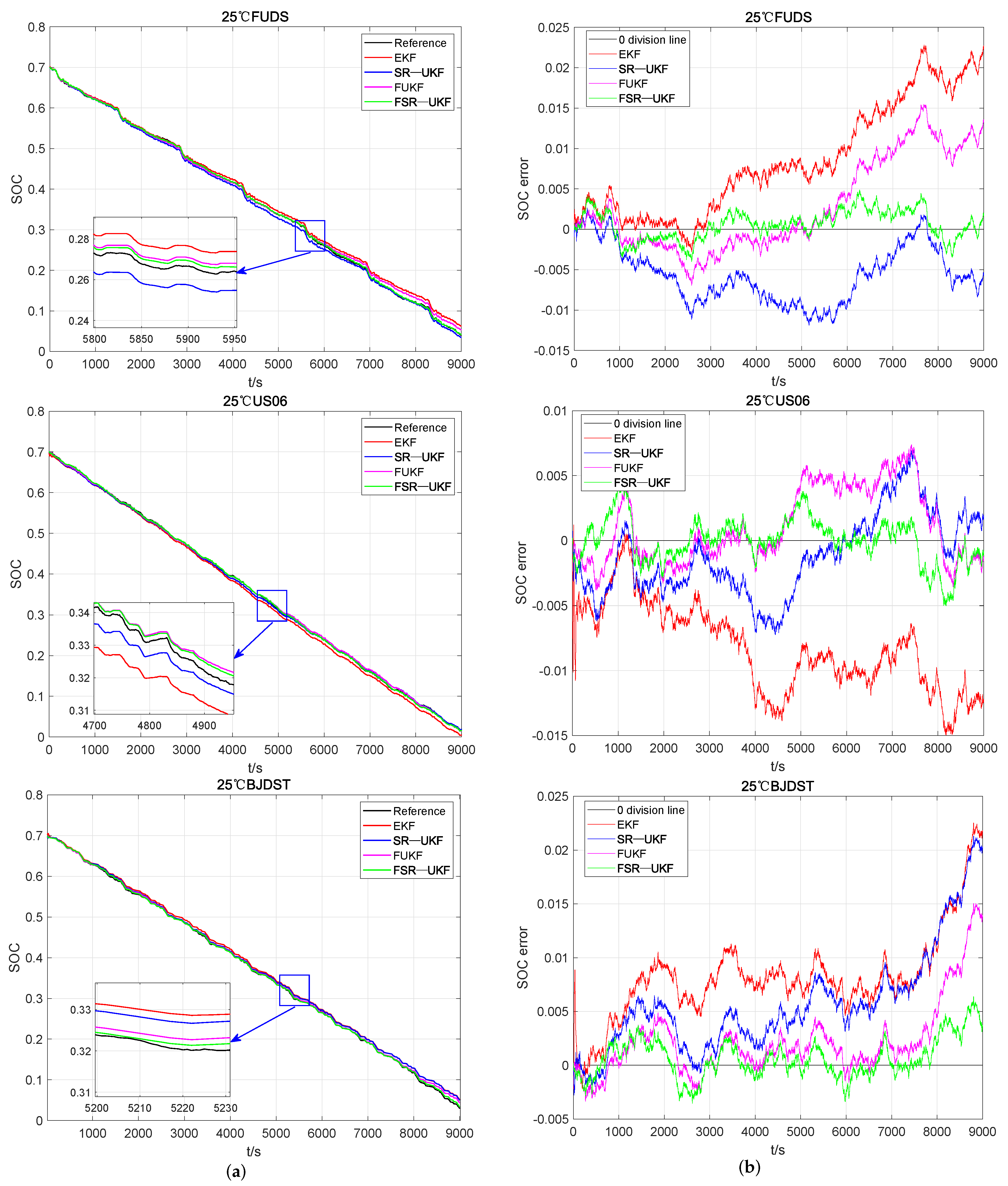
Uses the new SOC estimation method, yielding better results than other schemes, namely the EKF, SR-UKF, and FUKF, as shown by tests conducted under three different temperatures and three distinct working conditions.
The paper is organized as follows. Section 2 introduces the main concepts of fractional calculus that are used in the follow-up. Section 3 formulates the fractional second-order RC ECM of the lithium battery and presents the state-space equations. Section 4 discusses the parameter identification and the accuracy of the parameterized battery model. Section 5 and Section 6 analyze the FSR-UKF algorithm and its accuracy, respectively. Section 7 outlines the main conclusions.

2. Preliminaries

The Grünwald-Letnikov (GL), Riemann-Liouville, and Caputo definitions are common in fractional calculus. In this paper, the GL definition is adopted due to its straithforward application to the Kalman filtering [30]. As such we have:
a D t α x ( t ) = lim Δ T 0 1 ( Δ T ) α j = 0 [ t / Δ T ] ( 1 ) j α j x ( t j Δ T ) ,
where a D t α stands for the FO operator, a and t represent the lower and upper bounds of the operator, respectively, x ( t ) is a given function, Δ T denotes the sampling time, [ t / Δ T ] represents the memory length and
α j = Γ ( α + 1 ) Γ ( j + 1 ) Γ ( α j + 1 ) ,
where Γ ( α ) is the Gamma function, defined by:
Γ ( α ) = 0 + ξ α 1 e ξ d ξ .
The continuous-time GL derivative can be discretized with a fixed memory length L [15], yielding:
a D t α x k + 1 1 ( Δ T ) α x k + 1 + 1 ( Δ T ) α j = 1 L + 1 ( 1 ) j α j x k + 1 j .

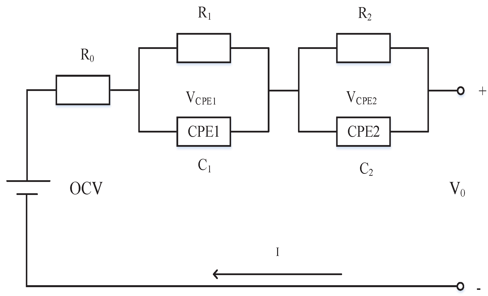
3. Fractional Order Modeling of Lithium-Ion Batteries

The electrochemical impedance spectroscopy (EIS) is an effective tool for determining the internal characteristics of lithium-ion batteries [31]. The process starts by applying to the device a low amplitude sine wave AC current x ( t ) , with different frequencies, and measuring the output AC signal y ( t ) , which has the same frequency as the input, but distinct amplitude, and phase. From the measurements, the transfer function G ( ω ) = Y ( ω ) / X ( ω ) can be obtained. The image of G ( ω ) in the complex plane represents the EIS characteristic of the lithium battery.
Figure 1 shows the Nyquist diagram of the battery obtained by the EIS procedure. We note the existence of three parts, namely the low-, intermediate- and high-frequency regions. The low-frequency region consists of a straight line with a fixed slope, representing the solid diffusion process of lithium ions inside the battery. We can use an RC branch to describe this part. The mid-frequency region is a semicircular area, which represents the charge transfer process. This part can be modeled by another RC branch. In the high-frequency region, the intersection of the impedance spectrum with the real axis corresponds to the ohmic internal resistance of the battery.
The second-order RC-ECM has been widely used to describe the behavior of lithium batteries. However, an ideal capacitor does not fully characterize the phenomena captured by the EIS. Instead of ideal capacitors, CPEs can be used. The complex impedance of a CPE is given by:
Z ( s ) = 1 C s α ,
where Z denotes the complex impedance, C is a constant representing the main capacitance effect, α denotes the FO, and s stands for the Laplace variable.
Hereafter, we will adopt the fractional second-order RC-ECM shown in Figure 2, where O C V represents the open-circuit voltage, R 0 is the ohmic internal resistance, R 1 and R 2 , and C 1 and C 2 denote the resistance and the capacitance in the two parallel branches, respectively, V 0 stands for the terminal voltage of the battery, and I corresponds to the current flowing through the circuit. The complex impedance values of the two CPEs are represented by Z C P E 1 ( s ) and Z C P E 2 ( s ) , that is:
Z C P E 1 ( s ) = 1 C 1 s α , Z C P E 2 ( s ) = 1 C 2 s β ,
where α , β ( 0 , 1 ) are the FO.
If we denote by V C P E 1 ( t ) and V C P E 2 ( t ) the voltages on the two parallel associations, respectively, then the equations of the dynamics are:
D α V C P E 1 ( t ) = V C P E 1 ( t ) R 1 C 1 + I ( t ) C 1 , D β V C P E 2 ( t ) = V C P E 2 ( t ) R 2 C 2 + I ( t ) C 2 .
Let us use Q n to denote the nominal capacity of the lithium battery, and η to represent the Coulomb efficiency. The SOC of the battery can be given by:
d ( SOC ( t ) ) d t = η Q n I ( t ) .
It follows from Kirchhoff’s voltage law that the terminals voltage V 0 ( t ) is given by:
V 0 ( t ) = O C V ( SOC ( t ) ) I ( t ) R 0 V C P E 1 ( t ) V C P E 2 ( t ) ,
where O C V is a nonlinear function of the SOC . The relationship between the O C V and the SOC is usually expressed as:
g [ θ ( t ) ] = O C V ( SOC ( t ) ) = k = 0 4 d k SOC k ( t ) ,
where d k ( k = 0 , , 4 ) are the coefficients of a polynomial. Equation (10) has been used in the literature to describe the O C V - SOC relationship [21,32].
Further, the state space equation of the lithium-ion battery can be written as,
D η x ( t ) = A x ( t ) + B u ( t ) , y ( t ) = C x ( t ) + D u ( t ) ,
where η = [ α , β , 1 ] T is the incommensurate vector, x ( t ) is the state vector, D η x ( t ) = [ D α V C P E 1 ( t ) , D β V C P E 2 ( t ) , D 1 SOC ( t ) ] T , u ( t ) denotes the system input (battery current I ( t ) ) and y ( t ) represents the system output (battery terminal voltage V 0 ( t ) ). The matrices A , B , C and D are obtained as:
A = 1 R 1 C 1 0 0 0 1 R 2 C 2 0 0 0 0 , B = 1 C 1 1 C 2 η Q n ,
C = 1 1 g [ θ ( t ) ] SOC ( t ) ,
D = R 0 .
With Equation (4) in mind, we can write model (11) in the discrete time:
x k + 1 = A 1 x k + B 1 u k j = 2 L + 1 ( 1 ) j γ j η x k + 1 j , : = f ( x k , u k ) j = 2 L + 1 ( 1 ) j γ j η x k + 1 j , y k = g ( θ k ) V C P E 1 k V C P E 2 k R 0 I k , : = h ( x k ) .
where f ( x k , u k ) stands for the system model, and h ( x k ) is the system measurement model. The matrices A 1 , B 1 and γ j η are as follows:
A 1 = d i a g ( ( Δ T ) α , ( Δ T ) β , ( Δ T ) ) A + d i a g ( α , β , 1 ) ,
B 1 = d i a g ( ( Δ T ) α , ( Δ T ) β , ( Δ T ) ) B ,
γ j η = d i a g α j , β j , 1 j .

4. Model Parameter Identification and Validation

4.1. Description of the Experimental Data

The current and voltage data of the battery INR 18650-20R, with a capacity of 2000 mAh, are provided by the CALCE Battery Research Group. We consider four current and voltage datasets for testing, which correspond to typical vehicle operating conditions [33]: Dynamic Stress Test (DST), Federal Urban Driving Schedule (FUDS), US06 Highway Driving Schedule (US06), and Beijing Dynamic Stress Test (BJDST). Their current and voltage profiles at the temperature of 25 C are shown in Figure 3. The current and voltage data at 0 C and 45 C, to be used in Section 5, can be found at the CALCE Battery Research Group (https://web.calce.umd.edu/batteries/index.html, accessed on 1 May 2020), being omitted here due to space constraints.

4.2. Parameter Identification

The current and voltage data under the DST conditions are used to identify the parameters of the model. The current and voltage data for the other three working conditions are used to verify the accuracy of the SOC estimation algorithm. Figure 3 shows that the DST is composed of several small cycles, each with a duration of 350 s [33]. Indeed, the DST consists of a variety of current steps with different amplitudes and lengths, and takes into account regenerative charging. In order to reduce the complexity of the analysis, we select one cycle for parameter identification. Figure 4 depicts the current and voltage data of a cycle, obtained from the 25 C DST dataset (data point ranging from 9430 to 9780), and with SOC values ranging from 0.549 to 0.575.
Online identification methods are more practical than their offline versions. An online method can simultaneously identify the parameters and estimate the SOC with a limited number of preliminary experiments. Meanwhile, the time-varying parameters of the lithium battery can be tackled efficiently. However, as pointed out in [22], FOMs adopt frequently off-line parameter identification methods, due to the additional complexity posed by the fractional calculus. Therefore, considering the complexity and computational burden involved, a particle swarm optimization (PSO) algorithm is employed to identify the parameters off-line. The PSO has the advantages of simplicity, fast convergence speed, and a limited number of variables.
Herein, the 12 parameters to be identified are d 0 , d 1 , d 2 , d 3 , d 4 , R 0 , R 1 , C 1 , R 2 , C 2 , α and β . In the process of parameter identification, we aim to minimize the root-mean-squared error (RMSE) between the measured and the estimated voltages. We define the objective function E as:
m i n E = k = 1 M [ V o ( k ) V ^ o ( k ) ] 2 ,
where V o ( k ) and V ^ o ( k ) represent the measured and estimated voltages, respectively, and M is the number of sampling points in the time response.
Table 1 shows the results of the parameter identification of the FOM. Since we intend to compare the FOM with the integer-order model, we perform also the identification of the parameters of the integer second-order RC-ECM under the same conditions used for the FOM. The number of parameters to be identified for the integer-order model are merely 10, since α and β are related just with the FOM. Table 2 lists the parameter identification results of the integer-order model.

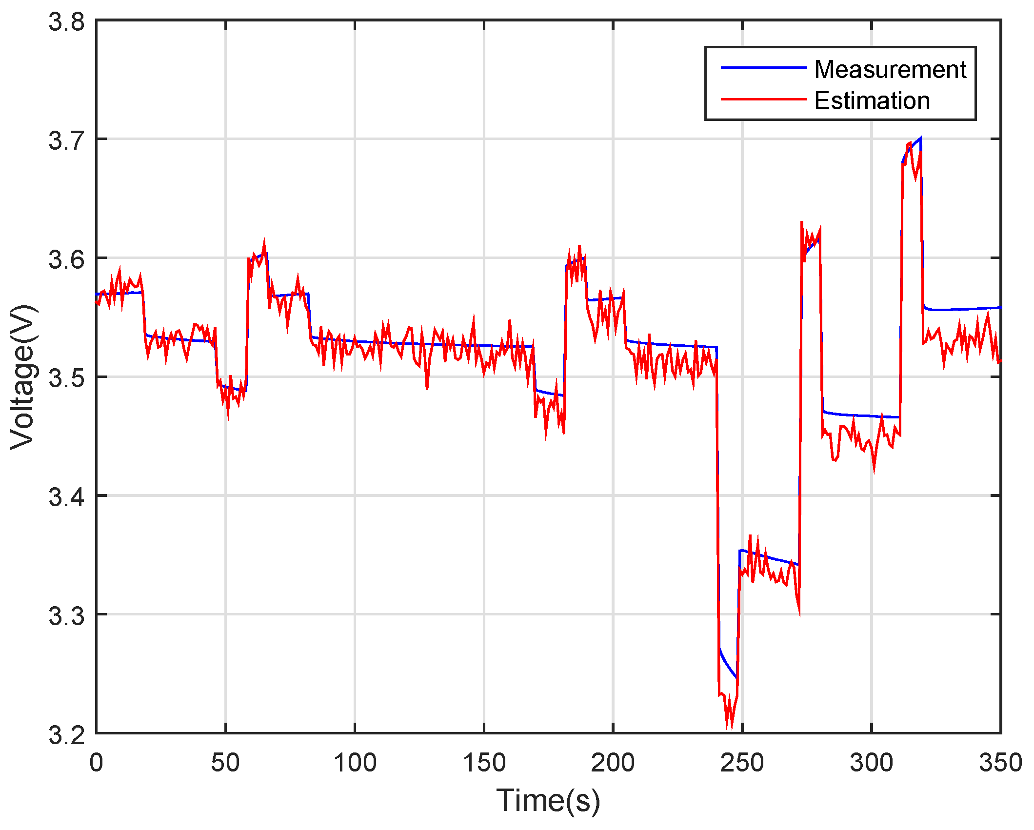
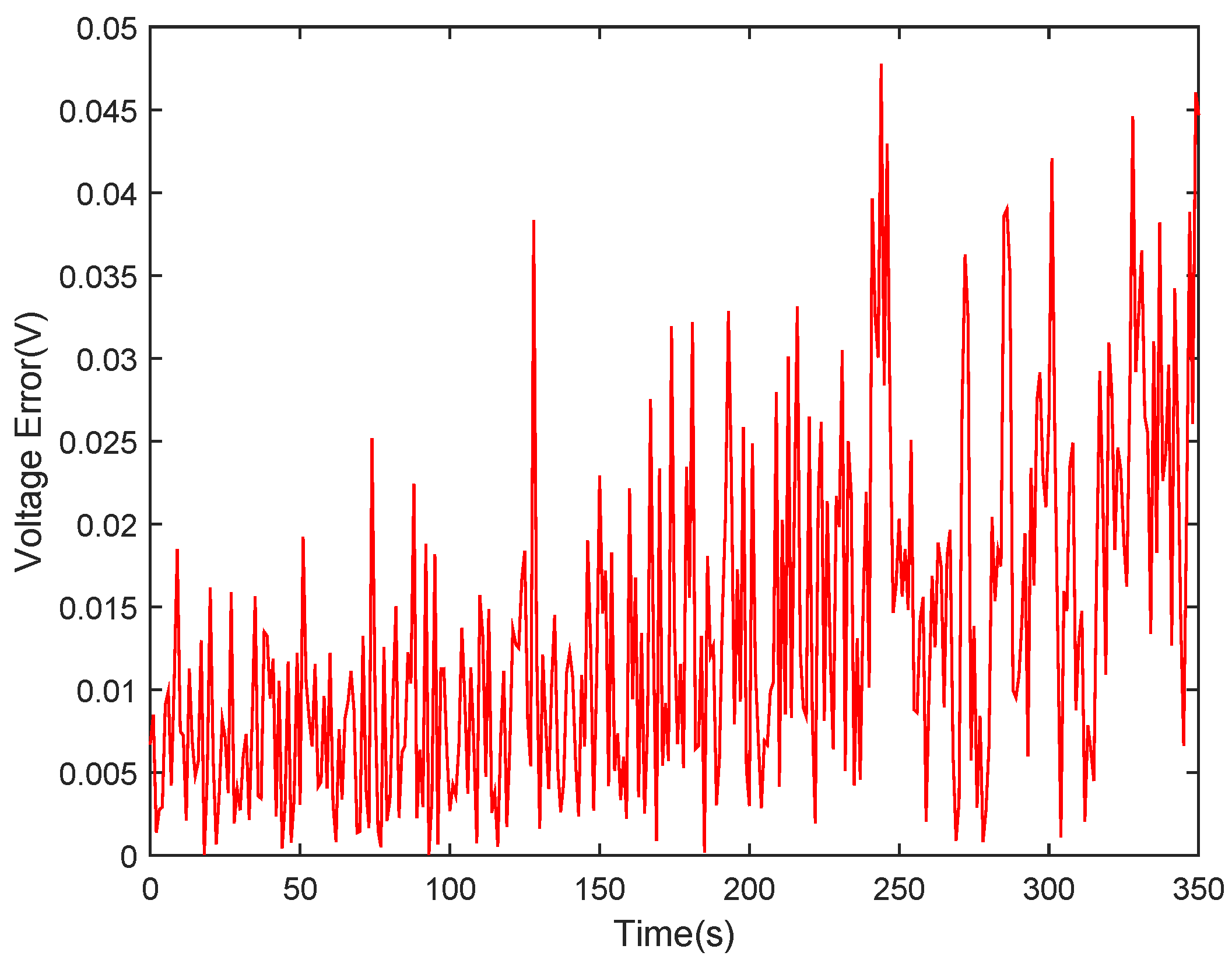
4.3. Model Accuracy Verification

The accuracy of the parameters identification method is important for characterizing the quality of the battery model. Figure 5 and Figure 6 show the accuracy for the FOM identification. We verify that (i) the maximum error is 33.23 mV, (ii) the error can be kept within 30 mV most of the time, and (iii) the RMSE is 11.6 mV. Therefore, the parameters identified are accurate, and characterize adequately the battery. Figure 7 and Figure 8 illustrate the accuracy of the parameters identification method of the integer-order model. We can see that (i) the maximum error is 47.75 mV, (ii) the RMSE is 16.7 mV, and (iii) the error is kept within 40 mV most of the time.
From Figure 5, Figure 6, Figure 7 and Figure 8, it is clear that the terminal voltage estimation error of the FOM is much smaller than the one exhibited by the integer-order model. In fact, we can say that it is the main reason why the SOC estimation of the FSR-UKF is better than that of the conventional SR-UKF.

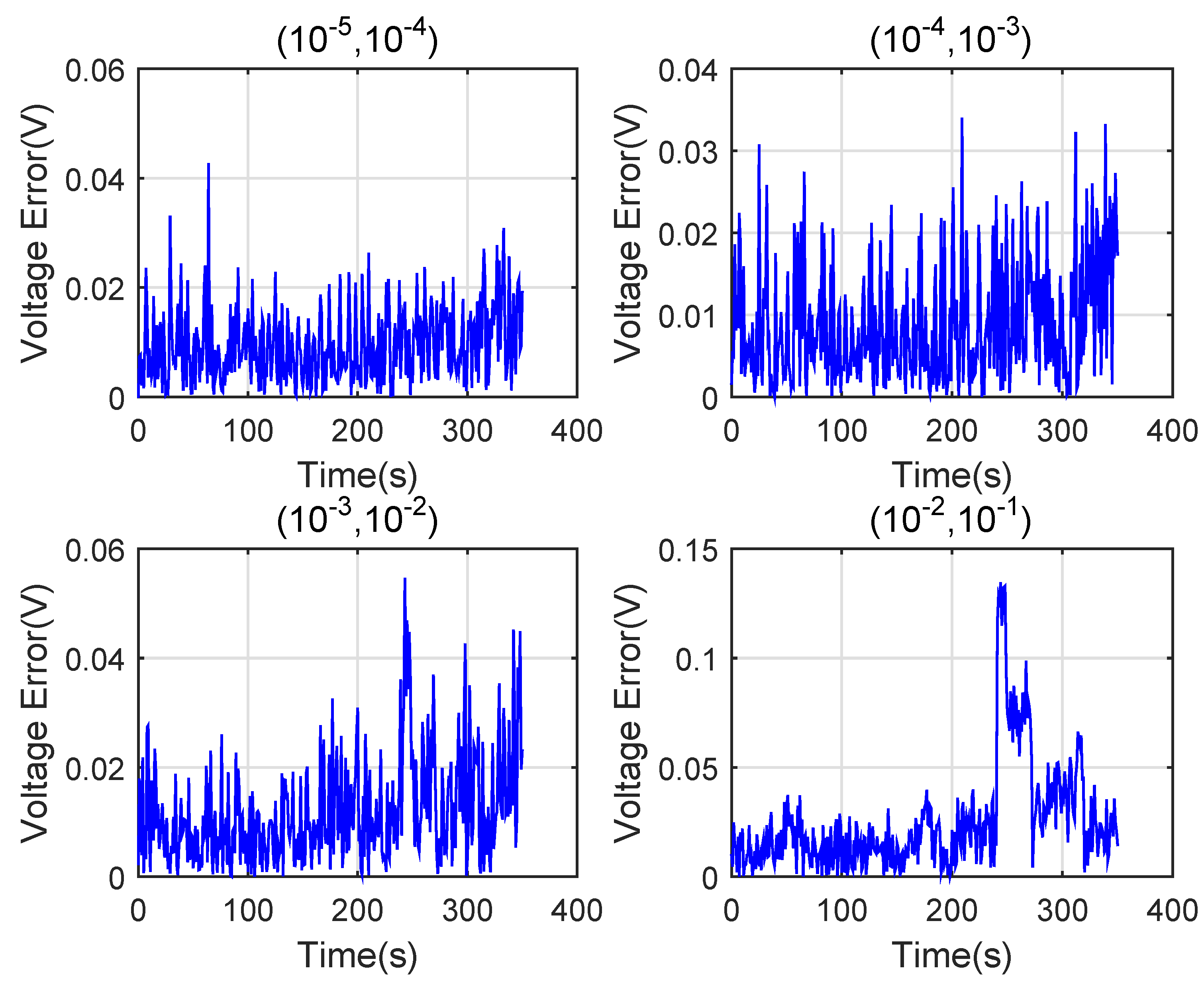
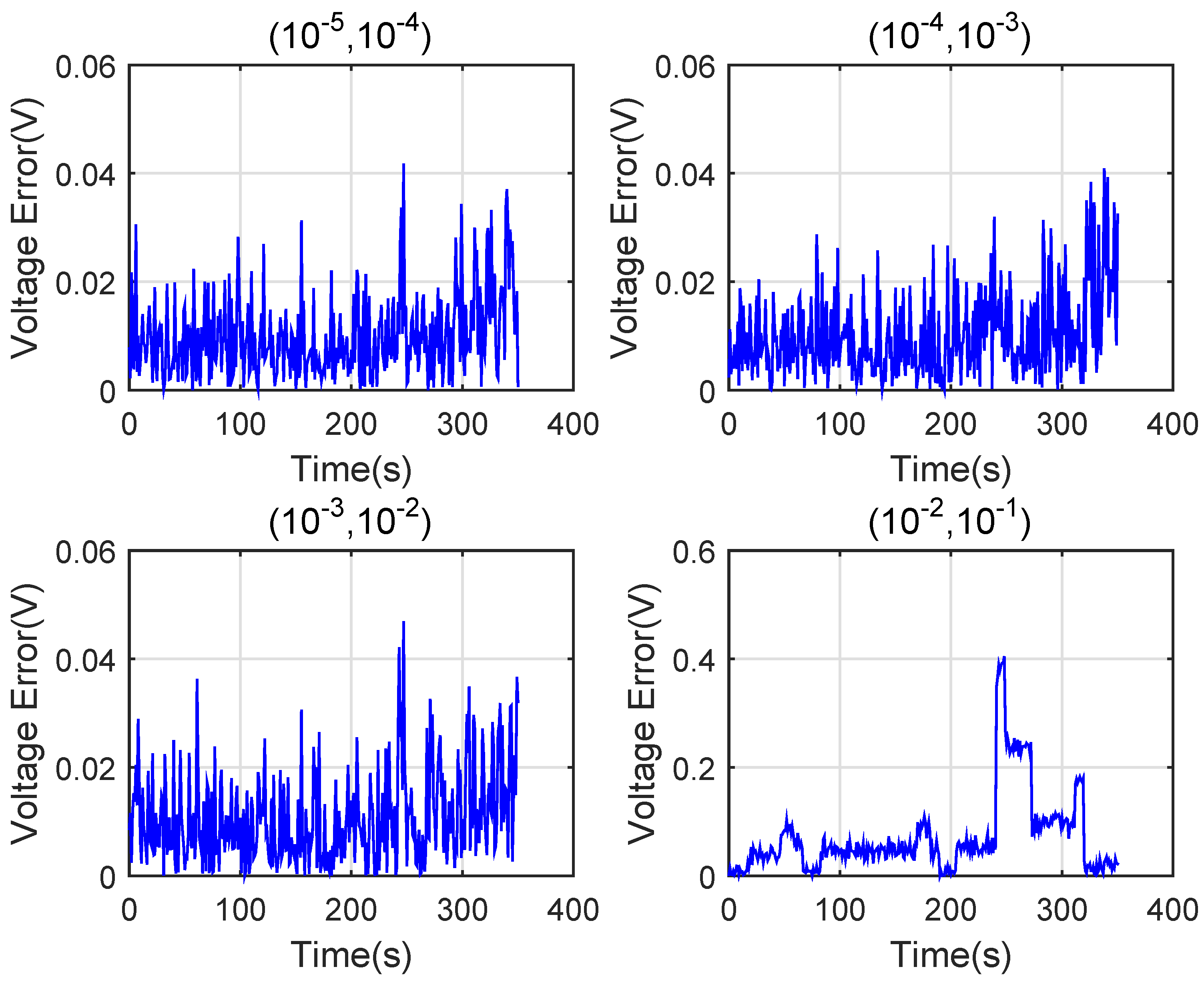
4.4. Model Parameters Sensitivity Analysis

The sensitivity analysis assesses the uncertainty in the output of a model with respect to the uncertainty in its input. After completing the parameter optimization phase, the sensitivity analysis is carried out to test the robustness of the values of the parameters. Herein, we analyze the 12 parameters of the lithium-ion battery FOM. We apply random noise in four ranges, namely [( 10 5 , 10 4 ), ( 10 4 , 10 3 ), ( 10 3 , 10 2 ), ( 10 2 , 10 1 )] to the parameters, and we assess their sensitivity in the perspective of the output voltage error. Three groups of experiments are carried out. The results are shown in Figure 9, Figure 10 and Figure 11. We verify that for the first three ranges of the noise, the model exhibits strong adaptability, and the output voltage error can be kept within 0.06 V. However, when the random noise perturbation is in the range ( 10 2 , 10 1 ) , their impact on the voltage error becomes serious. Therefore, we conclude that random noise below 10 2 has little effect on the accuracy of the model.

5. SOC Estimation

The integer-order UKF (IUKF) [34] and the FUKF [22,35] have been applied in the SOC estimation of lithium batteries. Similar to the evolution verified from the IUKF towards the FUKF, we can also think of the generalization of the integer-order SR-UKF to obtain the FSR-UKF. In other words, can the accuracy of the SOC estimation be improved using the FSR-UKF? In this perspective, a FSR-UKF method is proposed.
The FSR-UKF and the FUKF are based on FOMs of lithium-ion batteries. Note that the UKF usually suffers from the ill-conditioning of the covariance matrix, because the Cholesky decomposition requires a positive definite matrix during the iterations stage. However, this requirement may result in unsatisfied with an improper selection of the initial values. In contrast, the SR-UKF does not need decomposition and reconstruction of the covariance matrix, avoiding the re-factorization of the covariance matrix at each time step. Therefore, the positive semi-definiteness of the covariance matrix can be guaranteed. Herein, the FSR-UKF method is proposed by combining the advantages of the FOM and the SR-UKF.
Consider the following FO system:
D η x k + 1 = f ( x k , u k ) + ω k , x k + 1 = D η x k + 1 j = 2 L + 1 ( 1 ) j γ j η x k + 1 j , y k = h ( x k ) + υ k ,
where x k , u k and y k represent the state, input and output system variables, respectively. The variables ω k and υ k represent the Gaussian process and measurement noise, respectively. The symbols Q and H denote the covariance matrices of ω k and υ k , respectively.
The FSR-UKF algorithmic flow graph is shown in Figure 12. The detailed FSR-UKF steps are presented as follows:
(1)
Initialization
Specify the initial state x o , the matrices Q and H, and the initial state estimation error covariance P o . Set the Cholesky factor of the covariance P o as S o , and define S = c h o l ( P o ) ( c h o l represents the Cholesky decomposition).
(2)
Time updating
(a)
Calculate 2 n + 1 sigma sampling points:
ρ k 1 | k 1 = n + λ S k 1 | k 1 , x 0 , k 1 | k 1 = x ^ k 1 | k 1 , x i , k 1 | k 1 = x ^ k 1 | k 1 + ρ k 1 | k 1 j , i = 1 , 2 , , n , j = 1 , 2 , 3 , x i , k 1 | k 1 = x ^ k 1 | k 1 ρ k 1 | k 1 j , i = n + 1 , n + 2 , , 2 n , j = 1 , 2 , 3 ,
where n denotes the dimension of the system, and ρ k 1 | k 1 j is the jth column of ρ k 1 | k 1 . The weight of each sampling point is calculated as follows:
ω m o = λ n + λ , ω c o = λ n + λ + ( 1 α 1 2 + β 1 ) , ω m i = ω c i = 1 2 ( n + λ ) , i = 1 , 2 , , 2 n ,
where ω m i and ω c i are the weights of the mean of the sampling points and the covariance, respectively. The parameter λ = α 1 2 ( n + k ) n is a scaling factor that can be used to reduce the total prediction error of the system. The non-negative factor α 1 generally takes a small positive value to reduce the influence of the higher-order moments, and k is the turning parameter. The non-negative weight coefficient β 1 is used to reduce the peak error of the estimated state and to improve the accuracy of the covariance.
(b)
Propagate the sigma sampling points using the nonlinear function f ( · ) :
ϕ i , k | k 1 = f ( x i , k 1 | k 1 , u k 1 ) , i = 0 , 1 , 2 n , D η x ^ k | k 1 = j = 0 2 n ω m i ϕ i , k | k 1 .
(c)
Update the prior states estimation:
The square root mean and covariance propagation update is:
S k | k 1 Δ Δ = Q R ω c i ( ϕ 1 : 2 n , k | k 1 D η x ^ k | k 1 ) Q , S k | k 1 Δ Δ = C h o l u p d a t e ( S k | k 1 Δ Δ , ϕ 0 , k | k 1 D η x ^ k | k 1 , ω c 0 ) , S k | k 1 x Δ = j = 0 2 n ( x i , k 1 | k 1 x ^ k 1 | k 1 ) × ( ϕ 1 : 2 n , k | k 1 D η x ^ k | k 1 ) ,
where Q R denotes the Q R decomposition, and C h o l u p d a t e represents the Cholesky factor updating.
x ^ k | k 1 = D η x ^ k | k 1 j = 1 , k ( 1 ) j γ j x ^ k j | k j , S k | k 1 = S k | k 1 Δ Δ + γ 1 S k | k 1 x Δ + S k | k 1 Δ x γ 1 + j = 1 k γ j S k j | k j γ j .
(3)
Observation updating
(a)
Update the sigma points:
x 0 , k | k 1 = x ^ k | k 1 , x i , k | k 1 = x ^ k | k 1 + n + λ S k | k 1 , i = 1 , 2 , , n , x i , k | k 1 = x ^ k | k 1 n + λ S k | k 1 , i = n + 1 , n + 2 , , 2 n ,
where the weight remains equal to the one in Equation (22).
(b)
Propagate the sigma sampling points using the nonlinear measurement function h ( · ) :
θ i , k | k 1 = h ( x i , k | k 1 ) , i = 0 , 1 , , 2 n , y ^ k | k 1 = j = 0 2 n ω m i θ i , k | k 1 ,
(c)
Calculate the observation-error covariance matrix:
S k | k 1 y y = Q R ω c i ( θ 1 : 2 n , k | k 1 y ^ k | k 1 ) H , S k | k 1 y y = C h o l u p d a t e ( S k | k 1 y y , θ 0 , k | k 1 y ^ k | k 1 , ω c 0 ) ,
(d)
Compute the cross covariance matrix:
P k | k 1 x y = j = 0 2 n ω c i ( ϕ i , k | k 1 D η x ^ k | k 1 ) , × ( θ i , k | k 1 y ^ k | k 1 ) , i = 0 , 1 , , 2 n ,
(e)
Update the posterior states estimation:
K = P k | k 1 x y ( S k | k 1 y y ( S k | k 1 y y ) T ) 1 , x ^ k | k = x ^ k | k 1 + K ( y k y ^ k | k 1 ) , U = K S k | k 1 y y , S k | k = C h o l u p d a t e ( S k | k 1 , U , 1 ) .
We adopt an empirical trial and error method to find the best covariance matrix. The process noise covariance matrix Q represents the statistical characteristics of the model. If the value of Q increases, then the gain matrix and the correction weight also increase, improving the dynamic performance and stability of the algorithm. If the noise covariance H increases, then the gain matrix decreases, weakening the correction weight and compromising the transient and steady-state responses. Therefore, the effects of Q and H are opposite and their values should be selected according to the actual application. In what concerns the error covariance matrix P o , its size determines the amount of overshoot of the state estimate. A large P o leads to overshooting, but the estimated value evolves fast to the correct one. A small P o may result in a state estimate value that does not reach the correct one. Hereafter, we select Q = d i a g ( [ 10 8 , 10 8 , 10 8 ] ) , H = 10 2 and P o = d i a g ( [ 10 3 , 10 3 , 10 3 ] ) .

6. Simulation Verification and Discussion

In Section 4 we analyzed the current-voltage curves under four operating conditions at the temperature of 25 C. The current-voltage curve under DST conditions serves for parameter identification, while the other three are used to verify the accuracy of the SOC estimation.
Figure 13a shows the SOC estimation results under three operating conditions at 25 C. In all cases, the initial SOC values are selected equal to 0.7. Meanwhile, we choose the EKF, SR-UKF, and FUKF for comparison, in order to verify the FSR-UKF performance. The light green line is represented as the FSR-UKF. The red, blue, and magenta lines stand for EKF, SR-UKF, and FUKF, respectively. Also, the four algorithms are compared with the reference value represented by a black line. The closer to the reference, the higher the estimation accuracy of the algorithm. To allow good visualization of the experimental results, we use a partial magnification of the plot. Figure 13b shows the SOC estimation error associated to the EKF, SR-UKF, FUKF and FSR-UKF under the three operating conditions at 25 C. In order to improve the visualization of the magnitude of the estimation error, a 0 division line is added. It follows from Figure 13b that the estimation error of the EKF is the largest, followed by the ones of the SR-UKF and FUKF. On the other hand, the FSR-UKF maintains a high SOC estimation accuracy under all operating conditions.
The working environment of batteries poses some challenges, since frequently they have to operate in extreme temperatures. Therefore, the accuracy of the battery SOC estimation at extreme temperatures must be assessed. In order to verify the robustness of the FSR-UKF estimation method, we study the SOC both at low (0 C) and at high (45 C) temperatures.

6.1. Verification of the Algorithm at Low Temperatures 0 C

Figure 14a illustrates the SOC estimation results at 0 C when using the EKF, SR-UKF, FUKF and FSR-UKF, respectively. The initial SOC values under the three operating conditions are 0.7 , 0.75 , 0.7 , respectively. Figure 14a is partially magnified in order to highlight the differences. According to Figure 14a, one can see that the light green line, representing the FSR-UKF, is closer to the reference value, which also shows that the estimation accuracy of the FSR-UKF is higher. Figure 14b depicts the SOC estimation error. We verify that they are similar to those obtained at 25 C, and, consequently, the EKF, SR-UKF, and FUKF lead to higher estimation errors than the FSR-UKF. Most of the time, the estimation error of the FSR-UKF is kept within 0.005. The estimation errors of the other three algorithms are more than 0.005 most of the time. The FSR-UKF has small fluctuation, which shows that it can maintain good estimation accuracy and has certain stability even at low temperatures.

6.2. Verification of the Algorithm at High Temperatures 45 C

Figure 15a portraits the SOC estimation results under three operating conditions at 45 C. The initial values of the SOC are equal to 0.8. Figure 15a is also partially magnified so that we can more clearly observe which line is closer to the reference value represented by the black line. The SOC estimation errors are shown in Figure 15b. From Figure 15b, under the three working conditions, the SOC estimation error of our algorithm does not exceed 0.005 most of the time, but the estimation errors of the other three algorithms are much more than 0.005 and even 0.01. So we can verify that the FSR-UKF is better than the EKF, SR-UKF, and FUKF. The fluctuation of the FSR-UKF is smaller than that of the other three algorithms. This further verifies that our algorithm based on the FSR-UKF has certain stability at high temperatures. Therefore, both at low and high-temperature conditions, the proposed algorithm exhibits superior estimation accuracy.
Table 3, Table 4 and Table 5 list the RMSE values of the EKF, SR-UKF, FUKF and FSR-UKF estimation methods at the three temperatures (25 C, 0 C, 45 C). One can verify that the accuracy of the FSR-UKF is always superior to the one yielded by the other methods for all operating conditions (FUDS, US06, BJDST), and that its RMSE can always be kept within 1.0%.
From Figure 13, Figure 14 and Figure 15, we observe that the FUKF and FSR-UKF, which are based on FOMs, have smaller SOC estimation errors than the EKF and SR-UKF, which are based on integer-order models. The results prove that the FO filter methods surpass their integer-order versions. The results in Table 3, Table 4 and Table 5 show that the FSR-UKF exhibits always the smallest RMSE, which proves the effectiveness and robustness of the proposed strategy.

7. Conclusions

In this paper, a new FSR-UKF was proposed to estimate the SOC of lithium-ion batteries. The new strategy inherits the advantages of the SR-UKF, which does not require the reconstruction of the covariance matrix and, therefore, does not suffer from the ill-conditioning of that matrix, as occurs with the UKF. Moreover, the proposed method extends the SR-UKF to the FO domain, and takes full advantage of the fractional calculus to model the battery accurately. Simulation experiments were carried out at extreme temperatures (0 C and 45 C) for testing the effectiveness of the method. It was verified that the RMSE of the FSR-UKF can always be kept within 1%, demonstrating that the new scheme has good accuracy. In addition, tests with the EKF, SR-UKF, and FUKF showed the superiority of the proposed algorithm.

Author Contributions

Methodology, L.C.; software, X.W.; validation and data curation, X.D.; writing—original draft preparation, X.W.; writing—review and editing, A.M.L. and J.A.T.M.; supervision and project administration, P.L. We would like to dedicate this paper to J.A.T.M., who unfortunately passed away just before the paper was submitted for publication. J.A.T.M. played an essential role in the research described here and he is greatly missed. All authors have read and agreed to the published version of the manuscript.

Funding

This research was funded by the National Natural Science Funds of China (No. 62073114, No. 11971032), Ministry of Education China Mobile Research Fund (MCM20180404), Chongqing Basic Research and Frontier Exploration Project (cstc2018jcyjAX0167) and Chongqing Outstanding Youth Fund Project (cstc2021jcyj-jqx0001).

Data Availability Statement

The data that support the findings of this study are available which has included references to the CALCE article that describes the experiments conducted for generating the data.

Conflicts of Interest

The authors declare no conflict of interest.

References

  1. Saw, L.H.; Ye, Y.; Tay, A.A.O. Integration issues of lithium-ion battery into electric vehicles battery pack. J. Clean. Prod. 2016, 113, 1032–1045. [Google Scholar] [CrossRef]
  2. Diouf, B.; Pode, R. Potential of lithium-ion batteries in renewable energy. Renew. Energy 2015, 76, 375–380. [Google Scholar] [CrossRef]
  3. Xiong, R.; Li, L.; Tian, J. Towards a smarter battery management system: A critical review on battery state of health monitoring methods. J. Power Sources 2018, 405, 18–29. [Google Scholar] [CrossRef]
  4. Xiong, R.; Zhang, Y.; Wang, J.; He, H.; Peng, S.; Pecht, M. Lithium-ion battery health prognosis based on a real battery management system used in electric vehicles. IEEE Trans. Veh. Technol. 2019, 68, 4110–4121. [Google Scholar] [CrossRef]
  5. Li, P.; Zhang, Z.; Xiong, Q.; Ding, B.; Hou, J.; Luo, D.; Rong, Y.; Li, S. State-of-health estimation and remaining useful life prediction for the lithium-ion battery based on a variant long short term memory neural network. J. Power Sources 2020, 459, 228069. [Google Scholar] [CrossRef]
  6. Li, P.; Zhang, Z.; Grosu, R.; Deng, Z.; Hou, J.; Rong, Y.; Wu, R. An end-to-end neural network framework for state-of-health estimation and remaining useful life prediction of electric vehicle lithium batteries. Renew. Sustain. Energy Rev. 2022, 156, 111843. [Google Scholar] [CrossRef]
  7. Cheng, K.W.E.; Divakar, B.P.; Wu, H.; Ding, K.; Ho, H.F. Battery management system (BMS) and SOC development for electrical vehicles. IEEE Trans. Veh. Technol. 2011, 60, 76–88. [Google Scholar] [CrossRef]
  8. Zou, C.; Hu, X.; Wei, Z.; Tang, X. Electrothermal dynamics conscious Lithium-ion battery cell-level charging management via state monitored predictive control. Energy 2017, 141, 250–259. [Google Scholar] [CrossRef]
  9. Hu, X.; Li, S.; Peng, H. A comparative study of equivalent circuit models for Li-ion batteries. J. Power Sources 2012, 198, 359–367. [Google Scholar] [CrossRef]
  10. Seaman, A.; Dao, T.S.; Mcphee, J. A survey of mathematics-based equivalent-circuit and electrochemical battery models for hybrid and electric vehicle simulation. J. Power Sources 2014, 256, 410–423. [Google Scholar] [CrossRef] [Green Version]
  11. Nejad, S.; Gladwin, D.T.; Stone, D.A. A systematic review of lumped parameter equivalent circuit models for real-time estimation of lithium-ion battery state. J. Power Sources 2016, 316, 183–196. [Google Scholar]
  12. Huang, J.; Li, Z.; Liaw, B.Y.; Zhang, J. Graphical analysis of electrochemical impedance spectroscopy data in Bode and Nyquist representations. J. Power Sources 2016, 309, 82–98. [Google Scholar] [CrossRef]
  13. Zhou, X.; Huang, J.; Pan, Z.; Ouyang, M. Impedance characterization of lithium-ion batteries aging under high-temperature cycling: Importance of electrolyte-phase diffusion. J. Power Sources 2019, 426, 216–222. [Google Scholar] [CrossRef]
  14. Yang, Q.; Xu, J.; Cao, B.; Li, X. A simplified fractional order impedance model and parameter identification method for lithium-ion batteries. PLoS ONE 2017, 12, e0172424. [Google Scholar] [CrossRef]
  15. Zou, C.; Zhang, L.; Hu, X.; Wang, Z.; Wik, T.; Pecht, M. A review of fractional-order techniques applied to lithium-ion batteries, lead-acid batteries, and supercapacitors. J. Power Sources 2018, 390, 286–296. [Google Scholar] [CrossRef] [Green Version]
  16. Wang, B.; Li, S.E.; Peng, H.; Liu, Z. Fractional-order modeling and parameter identification for lithium-ion batteries. J. Power Sources 2015, 293, 151–161. [Google Scholar] [CrossRef]
  17. Wang, Y.; Chen, Y.; Liao, X. State-of-art survey of fractional order modeling and estimation methods for lithium-ion batteries. Fract. Calc. Appl. Anal. 2019, 22, 1449–1479. [Google Scholar] [CrossRef]
  18. Tian, J.; Xiong, R.; Shen, W.; Wang, J.; Yang, R. Online simultaneous identification of parameters and order of a fractional order battery model. J. Clean. Prod. 2019, 247, 119147. [Google Scholar] [CrossRef]
  19. Wang, Y.; Li, M.; Chen, Z. Experimental study of fractional-order models for lithium-ion battery and ultra-capacitor: Modeling, system identification, and validation. Appl. Energy 2020, 278, 115736. [Google Scholar] [CrossRef]
  20. Yu, M.; Li, Y.; Podlubny, I.; Gong, F.; Zhang, C. Fractional-order modeling of lithium-ion batteries using additive noise assisted modeling and correlative information criterion. J. Adv. Res. 2020, 25, 49–56. [Google Scholar] [CrossRef]
  21. Hu, X.; Yuan, H.; Zou, C.; Li, Z.; Zhang, L. Co-estimation of state of charge and state of health for lithium-ion batteries based on fractional-order calculus. IEEE Trans. Veh. Technol. 2018, 67, 10319–10329. [Google Scholar] [CrossRef]
  22. Xiong, R.; Tian, J.; Shen, W.; Sun, F. A novel fractional order model for state of charge estimation in lithium ion batteries. IEEE Trans. Veh. Technol. 2019, 68, 4130–4139. [Google Scholar] [CrossRef]
  23. Zhu, Q.; Xu, M.; Liu, W.; Zheng, M. A state of charge estimation method for lithium-ion batteries based on fractional order adaptive extended Kalman filter. Energy 2019, 187, 115880. [Google Scholar] [CrossRef]
  24. Mawonou, K.; Eddahech, A.; Dumur, D.; Beauvois, D.; Godoy, E. Improved state of charge estimation for Li-ion batteries using fractional order extended Kalman filter. J. Power Sources 2019, 435, 226710. [Google Scholar] [CrossRef]
  25. Gholizade-Narm, H.; Charkhgard, M. Lithium-ion battery state of charge estimation based on square-root unscented Kalman filter. IET Power Electron. 2013, 6, 1833–1841. [Google Scholar] [CrossRef]
  26. Aung, H.; Low, K.S. Temperature dependent state-of-charge estimation of lithium ion battery using dual spherical unscented Kalman filter. IET Power Electron. 2015, 8, 2026–2033. [Google Scholar] [CrossRef]
  27. Wang, K.; Feng, X.; Ren, J.; Duan, C.; Li, L. State of charge (SOC) estimation of lithium-ion battery based on adaptive square root unscented Kalman filter. Int. J. Electrochem. Sci. 2020, 15, 9499–9516. [Google Scholar]
  28. Jiang, C.; Wang, S.; Wu, B.; Fernandez, C.; Xiong, X.; Coffie-Ken, J. A state-of-charge estimation method of the power lithium-ion battery in complex conditions based on adaptive square root extended Kalman filter. Energy 2021, 219, 119603. [Google Scholar] [CrossRef]
  29. Aung, H.; Soon Low, K.; Ting Goh, S. State-of-Charge estimation of lithium-ion battery using square root spherical unscented Kalman filter (Sqrt-UKFST) in nanosatellite. IEEE Trans. Power Electron. 2015, 30, 4774–4783. [Google Scholar] [CrossRef]
  30. Monje, C.A.; Chen, Y.; Vinagre, B.M.; Xue, D.; Feliu-Batlle, V. Fractional-Order Systems and Controls: Fundamentals and Applications; Springer: London, UK, 2010. [Google Scholar]
  31. Waag, W.; Kaebitz, S.; Sauer, D.U. Application-specific parameterization of reduced order equivalent circuit battery models for improved accuracy at dynamic load. Measurement 2013, 46, 4085–4093. [Google Scholar] [CrossRef]
  32. Wang, B.; Liu, Z.; Li, S.E.; Moura, S.J.; Peng, H. State-of-Charge estimation for lithium-ion batteries based on a nonlinear fractional model. IEEE Trans. Control. Syst. Technol. 2017, 25, 3–11. [Google Scholar] [CrossRef]
  33. Zheng, F.; Xing, Y.; Jiang, J.; Sun, B.; Kim, J.; Pecht, M. Influence of different open circuit voltage tests on state of charge online estimation for lithium-ion batteries. Appl. Energy 2016, 183, 513–525. [Google Scholar] [CrossRef]
  34. Li, B.; Bei, S. Estimation algorithm research for lithium battery SOC in electric vehicles based on adaptive unscented Kalman filter. Neural Comput. Appl. 2018, 31, 8171–8183. [Google Scholar] [CrossRef]
  35. Chen, Y.; Huang, D.; Zhu, Q.; Liu, W.; Liu, C.; Xiong, N. A new state of charge estimation algorithm for lithium-ion batteries based on the fractional unscented Kalman filter. Energies 2017, 10, 1313. [Google Scholar] [CrossRef]
Figure 1. Nyquist diagram of a lithium battery.
Fractalfract 06 00052 g001
Figure 2. The ECM of a lithium battery.
Fractalfract 06 00052 g002
Figure 3. Current and voltage profiles of the DST (a), FUDS (b), US06 (c) and BJDST (d).
Fractalfract 06 00052 g003
Figure 4. Current and voltage data of a complete DST cycle.
Fractalfract 06 00052 g004
Figure 5. Accuracy verification of the FOM.
Fractalfract 06 00052 g005
Figure 6. Output terminals voltage error with the FOM.
Fractalfract 06 00052 g006
Figure 7. Accuracy verification of the integer-order model.
Fractalfract 06 00052 g007
Figure 8. Output terminals voltage error with the integer-order model.
Fractalfract 06 00052 g008
Figure 9. Sensitivity analysis of the model parameters (Group one).
Fractalfract 06 00052 g009
Figure 10. Sensitivity analysis of the model parameters (Group two).
Fractalfract 06 00052 g010
Figure 11. Sensitivity analysis of the model parameters (Group three).
Fractalfract 06 00052 g011
Figure 12. The FSR-UKF algorithmic flow graph.
Fractalfract 06 00052 g012
Figure 13. (a) The SOC estimation results of four algorithms under three operating conditions at 25 C. (b) The SOC estimation errors of four algorithms under three operating conditions at 25 C.
Fractalfract 06 00052 g013
Figure 14. (a) The SOC estimation results of four algorithms under three operating conditions at 0 C. (b) The SOC estimation errors of four algorithms under three operating conditions at 0 C.
Fractalfract 06 00052 g014
Figure 15. (a) The SOC estimation results of four algorithms under three operating conditions at 45 C. (b) The SOC estimation errors of four algorithms under three operating conditions at 45 C.
Fractalfract 06 00052 g015
Table 1. The results of the FOM parameter identification.
d 0 d 1 d 2 d 3 d 4 R 0
2.4877 1.8243 0.6608 1.1131 3.2348 0.0687
R 1 C 1 R 2 C 2 α β
0.5975264.251.2679448.540.43250.4380
Table 2. The results of the integer-order model parameter identification.
d 0 d 1 d 2 d 3 d 4
4.1498 1.1940 0.0907 0.6634 0.6488
R 0 R 1 C 1 R 2 C 2
0.07880.851392.650.533775.34
Table 3. The RMSE of four algorithms under three operating conditions at 25 C.
RMSEEKFSR-UKFFUKFFSR-UKF
FUDS1.09%0.66%0.64%0.19%
US060.89%0.34%0.31%0.17%
BJDST0.92%0.74%0.41%0.19%
Table 4. The RMSE of four algorithms under three operating conditions at 0 C.
RMSEEKFSR-UKFFUKFFSR-UKF
FUDS1.07%0.77%0.49%0.27%
US060.95%0.85%0.34%0.16%
BJDST0.50%0.42%0.40%0.21%
Table 5. The RMSE of four algorithms under three operating conditions at 45 C.
RMSEEKFSR-UKFFUKFFSR-UKF
FUDS0.93%0.61%0.61%0.22%
US060.93%0.82%0.70%0.23%
BJDST1.11%0.65%0.45%0.17%
Publisher’s Note: MDPI stays neutral with regard to jurisdictional claims in published maps and institutional affiliations.

