All articles published by MDPI are made immediately available worldwide under an open access license. No special
permission is required to reuse all or part of the article published by MDPI, including figures and tables. For
articles published under an open access Creative Common CC BY license, any part of the article may be reused without
permission provided that the original article is clearly cited. For more information, please refer to
https://www.mdpi.com/openaccess.
Feature papers represent the most advanced research with significant potential for high impact in the field. A Feature
Paper should be a substantial original Article that involves several techniques or approaches, provides an outlook for
future research directions and describes possible research applications.
Feature papers are submitted upon individual invitation or recommendation by the scientific editors and must receive
positive feedback from the reviewers.
Editor’s Choice articles are based on recommendations by the scientific editors of MDPI journals from around the world.
Editors select a small number of articles recently published in the journal that they believe will be particularly
interesting to readers, or important in the respective research area. The aim is to provide a snapshot of some of the
most exciting work published in the various research areas of the journal.
An option is the right to buy or sell a good at a predetermined price in the future. For customers or financial companies, knowing an option’s pricing is crucial. It is well recognized that the Black–Scholes model is an effective tool for estimating the cost of an option. The Black–Scholes equation has an explicit analytical solution known as the Black–Scholes formula. In some cases, such as the fractional-order Black–Scholes equation, there is no closed form expression for the modified Black–Scholes equation. This article shows how to find the approximate analytic solutions for the two-dimensional fractional-order Black–Scholes equation based on the generalized Riemann–Liouville fractional derivative. The generalized Laplace variational iteration method, which incorporates the generalized Laplace transform with the variational iteration method, is the methodology used to discover the approximate analytic solutions to such an equation. The expression of the two-parameter Mittag–Leffler function represents the problem’s approximate analytical solution. Numerical investigations demonstrate that the proposed scheme is accurate and extremely effective for the two-dimensional fractional-order Black–Scholes Equation in the perspective of the generalized Riemann–Liouville fractional derivative. This guarantees that the generalized Laplace variational iteration method is one of the effective approaches for discovering approximate analytic solutions to fractional-order differential equations.
The right to purchase or sell a basic product at a specific price in the future is known as an option. Options have a significant presence on marketplaces and exchanges. Determining the prices of an option is important for customers or financial companies. The valuation of options is one of the most important challenges in the field of financial investing. It is well known that the Black–Scholes model [1,2] is an effective instrument for figuring out an option’s cost. There are analytical and numerical approaches used by researchers to solve the Black–Scholes Equations [3,4,5,6,7,8,9,10].
We observe that the Black–Scholes Equations (1)–(3) are partial differential equations with integer-order derivatives. Further study [11,12,13,14] demonstrates that the globalized financial markets are fractal in nature. This illustrates that the traditional Black–Scholes model does not adequately reflect the actual financial market. Studies confirmed the applicability of fractional differential equations many years ago, demonstrating their usefulness for researching aspects linked to fractal geometry and fractal dynamics. Secondly, fractional differential equations provide several benefits in describing significant phenomena in a variety of disciplines, including electromagnetics, fluid flow, acoustics, electrochemistry, as well as material science [15,16,17,18]. Is it reasonable to use the fractional differential equation in the financial market? The answer to the question is “yes”. Fractional derivatives can be used in the financial market because they have a property called “self-similarity”. Further, fractional derivatives respond better to long-term repositories than integer order derivatives. The fractional derivative’s remarkable abilities are employed to solve the fractal complexity in the financial market. At the present, there is an increase in the number of publications that discuss the use of fractional calculus in financial theory [19].
The Black–Scholes equation with two assets of a European call option is defined by:
for (,, ) ∈ [0,∞ ) × [0,∞ ) × , with the terminal condition:
where u is the call option depending on the underlying asset prices , at time ;
, are the asset price variables;
, are the volatility function of underlying assets;
, are coefficients so that all risky asset price are at the same level;
is the volatility of and ;
r is the risk-free interest rate;
T is the expiration date;
where is strike price of the ith underlying asset.
K. Trachoo, W. Sawangtong, and P. Sawangtong [20] researched the two-dimensional Black–Scholes equation with European call option (1) and (2) in 2017. Using the Laplace transform homotopy perturbation approach, they demonstrated that the explicit solution to this issue is represented as a Mellin–Ross function.
P. Sawangtong, K. Trachoo, W. Sawangtong, and B. Wiwattanapataphee [21] investigated the modified Black–Scholes model of (1) and (2) with two assets based on the Liouville–Caputo fractional derivative in 2018. They established, using the Laplace transform homotopy perturbation technique, that the explicit solution to this problem is represented as the Generalized Mittag–Leffler function.
2. The Modified Black–Scholes Equation
The modified Black–Scholes equation in fractional-order derivative form is presented in this section. Let and Readers may find out more information for transformation in [21]. Without loss of generality, we consider the variables x and y by and where and are positive constants. In the end, the Black–Scholes partial differential equation with two assets of the European call option Equations (1) and (2) is capable of being converted into the following form:
with the initial condition:
where and are constants defined by
In this study, we extend the previous work [20] and analyze the general form of the Black–Scholes equation in Equations (3) and (4) by replacing the integer-order time derivative with the fractional-order time derivative. The fractional-order Black–Scholes equation based on the generalized Riemann–Liouville fractional derivative with is considered in the form:
with the fractional integral initial condition:
where , and denote the generalized Riemann–Liouville fractional-order derivative with order and the generalized fractional-order integral with order , respectively.
The generalized Laplace variational iteration method is a methodology combining the variational iteration approach with the generalized Laplace transform. Analytical solutions are more complex to obtain than numerical solutions, particularly for fractional partial differential equations. Consequently, the analytical solution offers a valuable instrument for analyzing financial behavior. The generalized Laplace variational iteration approach is used in this research to provide the approximate analytic solution of the time fractional-order Black–Scholes model with two assets for the European call option (6) and (7). In addition, the closed-form analytic solution of the fractional-order Black–Scholes model (6) and (7) is investigated under certain requirements.
The structure of the article is as follows. The definitions of the generalized fractional-order derivative and integral are presented in Section 3. Section 4 discusses the generalized Laplace variational iteration technique’s application and convergence analysis. The explicit solution of the fractional-order Black–Scholes equation is provided in Section 5. In Section 6, numerical results with various parameter values can be seen. This work’s conclusion is provided into Section 7.
3. Basic Definitions
In this section, the generalized Riemann–Liouville fractional integral, the generalized Riemann–Liouville fractional derivative, and the generalized Laplace transform with their some properties have been discussed. For more details, readers can see [22,23]. Throughout this article, we assume that and are constants with and and we denote the gamma function by .
Definition 1.
The generalized fractional-order integral α of a continuous function is expressed as
Definition 2.
The generalized Riemann–Liouville fractional-order derivative of α of a continuous function is given as
We next give some properties that deal with the generalized Riemann–Liouville fractional derivative.
Lemma1.
Let be a continuous function and c be a constant. Then,
,
The following part discusses the generalized Laplace transform and some of its properties.
Definition 3.
The generalized Laplace transform of a continuous function is defined as
where s is the Laplace transform parameter.
It is important to note that the generalized Laplace transform can be reduced to the Laplace transform when .
Lemma2.
Let be a continuous function and c be a constant. Then,
.
Definition 4.
Let and be continuous functions. The generalized convolution of f and g is defined by
if the integral exists.
Lemma 3.
Let and be continuous functions. If and exist, then
In the last part of this section, we will introduce a special function that helps us rewrite complex expressions in a simple form.
Definition 5.
The two-parameter Mittag–Leffler function is defined as follows:
where Γ denotes the Gamma function, and
It is important to note that,
4. The General Methodology of the Generalized Laplace Variational
Iteration Method
In this section, we apply the generalized variational iteration method to the nonlinear partial differential equation. Assume that is the bounded domain. Let us consider the following general fractional differential equation in the generalized Riemann–Liouville fractional derivative
and the generalized Riemann–Liouville fractional initial condition
where and are the generalized Riemann–Liouville fractional derivative and integral of order respectively, is a linear term, is a nonlinear term and f and g are given functions.
In the first step of the process, we find the suitable Lagrange multiplier that will be found by using properties of the generalized Riemann–Liouville fractional derivative and integral.
Based on the generalized Riemann–Liouville integration, the correction functional for the nonlinear problem (8) and (9) is defined by
4.1. Lagrange Multipliers
Theorem 1.
The Lagrange multiplier λ for the fractional-order nonlinear partial differential Equations (8) and (9) can be determined by .
Proof.
Let us consider the correction functional (10) for the nonlinear problem (8) and (9):
Let . Thus,
where is the generalized convolution of a and . The generalized Laplace variational iteration correction functional will be defined in the following manner:
or equivalenty, upon applying the properties of the Laplace transform, we have
Taking the variation with respect to of both side of the latter equation, leads to
and upopn simplification we obtain
Furthermore, the extra condition of requires that . Moreover, the terms and are considered as restricted variations, which implies and . We then obtain or
The inverse generalized Laplace transform implies that
By the definition of a, the Lagrange multipliers is □
Note that it follows form Theorem 1 that the correction functional (10) associated with (8) and (9), is formed as:
4.2. Convergence Analysis of the Proposed Method
In this section, we study the convergence of the generalized Laplace variational iteration method, when applied to the nonlinear partial differential Equations (8) and (9). The sufficient conditions for convergence of the method and the error estimate are presented. The main results are proposed in the below theorems.
We next define the operator , where is the domain of the operator A and is a Banach space, by:
and define the sequence by:
The relationship between the sequences and given by (10) and (12), respectively, is shown in the following lemma.
Lemma 4.
Let and be the sequences constructed by (10) and (12), respectively. Then, for any
Proof.
We can deduce from (10) and (12) that and This implies that
We also know that from (10) and (12), and . By (13), we then get
Once again, we find that and . This yields, by (13) and (14), that Throughout this procedure, we finally discover that that for any This will lead to the desired results. □
It is important to note that, if the limit exists, Lemma 4 enables us to get that
The next lemma shows the convergence of the infinite series
Lemma 5.
Assume that there exists a positive real number γ with such that for any Then, the infinite series given by (12) converges.
Proof.
Let denote the partial sum of the infinite series We would like to show that the sequence is a Cauchy sequence in the Banach space It follows from the assumption of the theorem that we have:
Let n and m be any natural numbers with . We consider that by (15):
We can deduce from the fact that that:
Therefore, is a Cauchy sequence in the Banach space This information indicates that the infinite series determined by (12) converges in the Banach space Hence, Lemma 1 is proved completely.
The below theorem demonstrates that the convergent series is the solution of the nonlinear Equations (8) and (9). □
Lemma 6.
Let be the function such that the infinite series , determined by (12), converges to Then, the function is the solution of the nonlinear partial differential Equations (8) and (9) for any .
Proof.
By the property of the convergent series , we get that Let us consider the following:
and
Taking the generalized Riemann–Liouville fractional derivative on both sides of (17), we find that:
It follows from (11) and (12) and the linearity property of operators that we obtain:
This information implies is the infinite series solution of the nonlinear partial differential Equations (8) and (9). □
Lemma 7.
Assume that the infinite series , where is defined by (12), converges to the solution u of the nonlinear partial differential Equations (8) and (9). If the approximate analytic solution is the truncated series constructed by for any , then the maximum error norm can be evaluated as
where γ is the real number given in Lemma 5.
Proof.
Let n and M be any natural numbers with . As discussed in Theorem 1, we obtain that:
where is the partial sum of the infinite series As we let approach to infinity, we obtain that:
The definition of real number implies that and
The proof of Lemma 7 is therefore complete. □
The following main theorem is the result from Lemmas 5 and 6.
Theorem 2.
By using the generalized Laplace variational iteration approach, the approximate analytic solution for the general fractional differential Equation (8) with the integral initial condition (9) can be obtained by the following iteration:
for any and for all . Moreover, if exists, then the analytic solution u for the general fractional differential Equation (8) with the integral initial condition (9) can be found by
5. An Application of the Generalized Laplace Variational Iteration Method
In this part, we will apply the generalized Laplace variational iteration method to the fractional-order Black–Scholes equation based on the generalized Riemann–Liouville fractional derivative with the fractional integral initial condition (6) and (7). By (8) and (9), we set that , , and By Theorem 2 and by choosing
We obtain that:
Note that The generalized Laplace transform is then used to aid us discover the terms for . Let us consider the following:
Taking the generalized Laplace transform on both sides of the above equation:
The inverse generalized Laplace transform yields that
for Thus, the generalized Laplace variational iteration method for finding the approximate analytic solution of the fractional-order Black–Scholes Equation (6) with the fractional integral condition (7) is defined by:
with for all
Theorem 3.
The approximate analytic solution for the two dimensional fractional-order Black–Scholes Equation (6) with the fractional integral condition (7) can be defined by the following iteration:
for any and for all Furthermore, if
approaches zero when n goes to infinity for any fixed , then the analytic solution u for the fractional-order Black–Scholes Equations (6) and (7) is in the form:
where denotes the two-parameter Mittag–Leffler function.
Proof.
Let The generalized Laplace variational iteration procedure is then started by computing the term By (22), we obtain:
Then, the function is
Note that the function satisfies that We next find the function By (22), we get:
Consider
Then, the term is determined by
Note that the function satisfies that As a result of the preceding explanation, we now have term as follows:
Note that the function satisfies that Using the same manner, we can find the expression of in the following form:
and for all As a consequence of the generalized Laplace variational iteration process, we derive that, under the assumption of the theorem, the analytic solution for the fractional Black–Scholes equation is as follows:
Therefore, the Theorem 3 is proved completely. □
Corollary 1.
The analytic solution for the two-dimensional fractional-order Black–Scholes equation based on the Riemann–Liouville fractional derivative with the Riemann–Liouville fractional integral condition is given in the following:
for any
Proof.
By setting , this corollary can be obtained immediately from Theorem 3. □
Corollary 2.
The analytic solution of the classical two-dimensional Black–Scholes equation with the European call option is:
for any
Proof.
By Theorem 3, we have that
Since the generalized Riemann–Liouville fractional derivative can be reduced to the usual derivative when we obtain:
for any □
6. Numerical Results
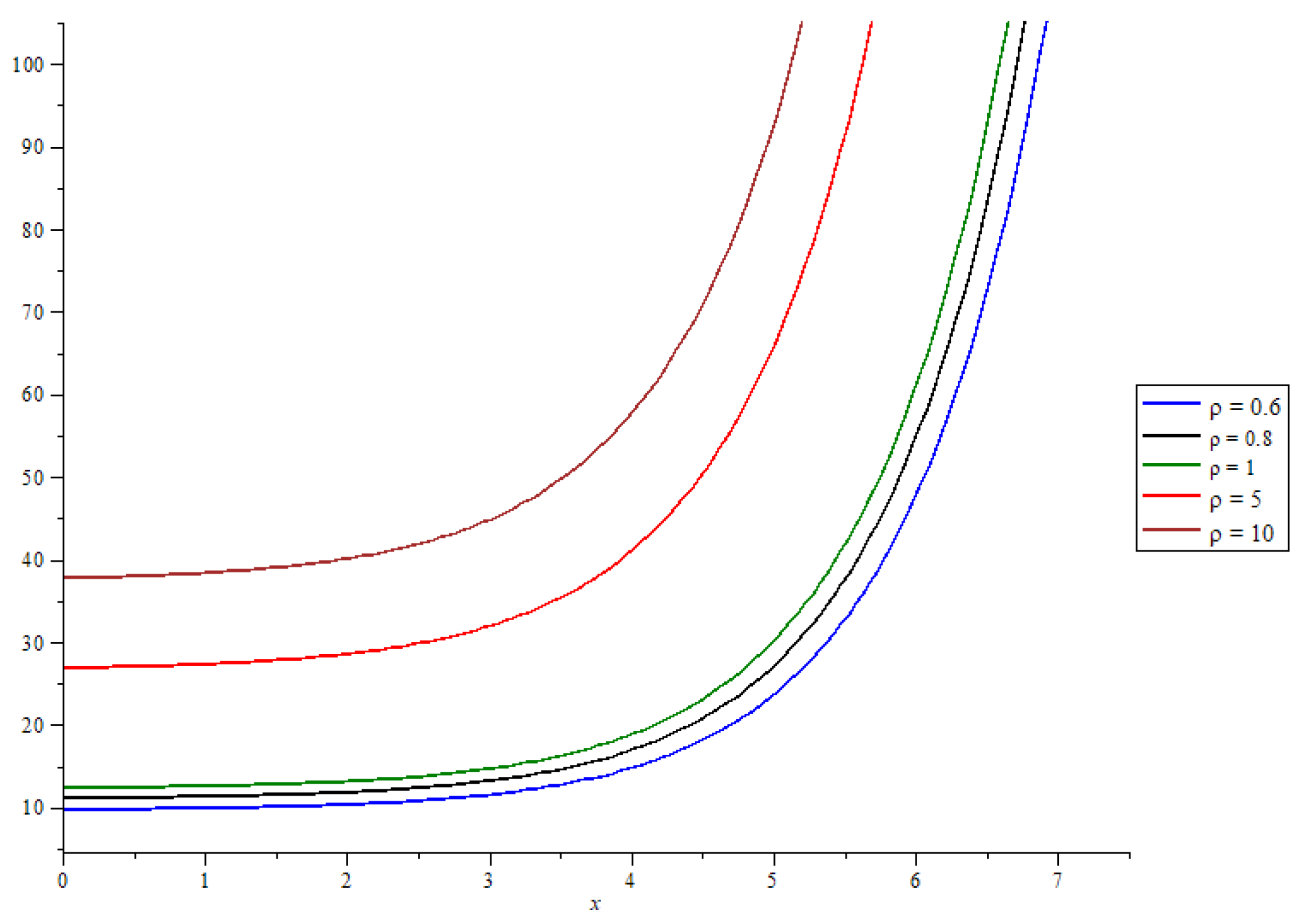
We will assume throughout this section that the strike price K is The risk-free annual interest rate is thus the maturity time is year; and the volatilities of the underlying assets and are and , respectively. In the following, we will demonstrate the European option prices computed from the previously described analytic solutions. Figure 1 shows the European call-option pricing with various values of the parameter obtained by (24) with the asset pricing and .
Figure 2 demonstrates the European call-option pricing with various values of the parameter given by (24) with the asset pricing and .
In case , the graphs of the option pricing by (24) with four different values for fractional order and are shown in Figure 3.
It is well known that in the classical Black–Scholes model, the option price depends on five variables. These are volatility, the price of the underlying asset, the strike price of the option, the time until expiration of the option, and the risk-free interest rate. With these variables, sellers of options could, in theory, set prices for the options they sell that make sense. However, in the fractional-order Black–Scholes equation proposed here, there are two parameters added: and . In each of the figures, it is shown that the value of call options will increase according to the values of two parameters. Therefore, if we can figure out the right values for these two factors, the modified Black–Scholes equation will give us option prices that are close to what they are worth on the market.
7. Conclusions
It is well known that in option pricing theory, the Black–Scholes equation is one of the most significant models for option pricing. In this manuscript, we developed the classical Black–Scholes equation in the form of the fractional-order Black–Scholes equation based on the generalized Riemann–Liouville derivative. This article provides the approximate analytic solution to the fractional-order Black–Scholes equation via the generalized Laplace variational iteration method. Moreover, we show that the solution to the classical Black–Scholes equation is achieved as a special case of the proposed approximate analytic solution. This demonstrates that the generalized Laplace variational iteration method is one of the effective approaches for discovering approximate analytic solutions to fractional-order differential equations. The advantage of the modified Black–Scholes equation is that it has two parameters occurring in the definition of the fractional derivative, that is and If we can correctly estimate the values of these two factors, the option prices produced from the modified form will be close to the market value of option prices. We may utilize the genetic algorithm and the actual value of the option to determine the proper values for two parameters. Option pricing may be determined by the solution to the modified Black–Scholes equation after the proper values for these two parameters are already known.
Author Contributions
Conceptualization, P.S.; Formal analysis, S.A., P.S. and W.S.; Investigation, P.S.; Methodology, S.A. and W.S.; Software, S.A., P.S. and W.S.; Supervision, P.S.; Writing—original draft, S.A.; Writing—review & editing, P.S. and W.S. All authors have read and agreed to the published version of the manuscript.
Funding
This research was funded by King Mongkut’s University of Technology North Bangkok, contract no. KMUTNB-FF-65-58.
Data Availability Statement
Not applicable.
Conflicts of Interest
The authors declare no conflict of interest.
References
Stampái, J.; Victor, G. The Mathematics of Finance: Modeling and Hedging; Books/Cole Series in Advanced Mathematics; Books/Cole: Pacific Grove, CA, USA, 2001. [Google Scholar]
Wilmott, P.; Howison, S.; Dewynne, J. The Mathematics of Financial Derivatives; Cambridge University Press: Cambridge, UK, 1997. [Google Scholar]
Topper, J. Financial Engineering with Finite Elements; John Wiley & Sons: Hoboken, NJ, USA, 2008. [Google Scholar]
Wilmott, P.; Dewynneand, J.; Howisson, S. Option Pricing: Mathematical Models and Computation; Oxford Press: Oxford, UK, 1993. [Google Scholar]
Seydel, R. Tools for Computational Finance; Springer: Berlin/Heidelberg, Germany, 2003. [Google Scholar]
Achdou, Y.; Olivier, P. Computational Methods for Option Pricing; Society for Industrial and Applied Mathematics: Philadelphia, PA, USA, 2005. [Google Scholar]
Mrazek, M.; Pospisil, J.; Sobotka, T. On calibration of stochastic and fractional stochastic volatility models. Eur. J. Oper. Res.2016, 254, 1036–1046. [Google Scholar] [CrossRef]
Alghalith, M. Pricing the American options using the Black-Scholes pricing formula. Physica A2018, 507, 443–445. [Google Scholar] [CrossRef]
Laskin, N. Valuing options in shot noise market. Physica A2018, 502, 518–533. [Google Scholar] [CrossRef]
Lin, L.; Li, Y.; Wu, J. The pricing of European options on two underlying assets with delays. Physica A2018, 495, 143–151. [Google Scholar] [CrossRef]
Mandelbrot, B. The variation of certain speculative prices. J. Bus.1963, 36, 394–413. [Google Scholar] [CrossRef]
Peters, E.E. Fractal structure in the capital markets. Financ. Anal. J.1989, 45, 32–37. [Google Scholar] [CrossRef]
Li, H.Q.; Ma, C.Q. An empirical study of long-term memory of return and volatility in Chinese stock market. J. Financ. Econ.2005, 31, 29–37. [Google Scholar]
Huang, T.F.; Li, B.Y.; Xiong, J.X. Test on the chaotic characteristic of Chinese futures market. Syst. Eng.2012, 30, 43–53. [Google Scholar]
Debnath, L. Recent applications of fractional calculus to science and engineering. Int. J. Math. Math. Sci2003, 2003, 753601. [Google Scholar] [CrossRef] [Green Version]
He, J.H.; El-Dib, Y.O. Periodic property of the time-fractional Kundu–Mukherjee–Naskar equation. Results Phys.2020, 19, 103345. [Google Scholar] [CrossRef]
Noeiaghdam, S.; Dreglea, A.; He, J.; Avazzadeh, Z.; Suleman, M.; Fariborzi Araghi, M.A.; Sidorov, D.N.; Sidorov, N. Error Estimation of the Homotopy Perturbation Method to Solve Second Kind Volterra Integral Equations with Piecewise Smooth Kernels: Application of the CADNA Library. Symmetry2003, 12, 1730. [Google Scholar] [CrossRef]
Anjum, N.; He, J.H. Higher-order homotopy perturbation method for conservative nonlinear oscillators generally and microelectromechanical systems’ oscillators particularly. Int. J. Mod. Phys. B2020, 34, 2050313. [Google Scholar] [CrossRef]
Song, L. A semianalytical solution of the fractional derivative model and its application in financial market. Complexity2018, 2018, 1872409. [Google Scholar] [CrossRef]
Trachoo, K.; Sawangtong, W.; Sawangtong, P. Laplace transform homotopy perturbation method for the two dimensional Black Scholes model with European call option. Math. Comput. Appl.2017, 22, 23. [Google Scholar] [CrossRef] [Green Version]
Sawangtong, P.; Trachoo, K.; Sawangtong, W.; Wiwattanapataphee, B. The analytical solution for the Black-Scholes equation with two assets in the Liouville-Caputo fractional derivative sense. Mathematics2018, 6, 129. [Google Scholar] [CrossRef]
Udita, N.K. A new approach to generalized fractional derivatives. Bull. Math. Anal. Appl.2014, 6, 1–15. [Google Scholar]
Jarad, F.; Abdeljawad, T. A modifi ed Laplace transform for certain generalized fractional operators. Results Nonlinear Anal.2018, 1, 88–98. [Google Scholar]
Figure 1.
European call-option prices with various fractional-order values.
Figure 1.
European call-option prices with various fractional-order values.
Figure 2.
European call-option prices with various fractional-order values.
Figure 2.
European call-option prices with various fractional-order values.
Figure 3.
The graphs of the option pricing with different fractional-order .
Figure 3.
The graphs of the option pricing with different fractional-order .
Publisher’s Note: MDPI stays neutral with regard to jurisdictional claims in published maps and institutional affiliations.
Ampun, S.; Sawangtong, P.; Sawangtong, W.
An Analysis of the Fractional-Order Option Pricing Problem for Two Assets by the Generalized Laplace Variational Iteration Approach. Fractal Fract.2022, 6, 667.
https://doi.org/10.3390/fractalfract6110667
AMA Style
Ampun S, Sawangtong P, Sawangtong W.
An Analysis of the Fractional-Order Option Pricing Problem for Two Assets by the Generalized Laplace Variational Iteration Approach. Fractal and Fractional. 2022; 6(11):667.
https://doi.org/10.3390/fractalfract6110667
Chicago/Turabian Style
Ampun, Sivaporn, Panumart Sawangtong, and Wannika Sawangtong.
2022. "An Analysis of the Fractional-Order Option Pricing Problem for Two Assets by the Generalized Laplace Variational Iteration Approach" Fractal and Fractional 6, no. 11: 667.
https://doi.org/10.3390/fractalfract6110667
Article Metrics
No
No
Article Access Statistics
For more information on the journal statistics, click here.
Multiple requests from the same IP address are counted as one view.
Ampun, S.; Sawangtong, P.; Sawangtong, W.
An Analysis of the Fractional-Order Option Pricing Problem for Two Assets by the Generalized Laplace Variational Iteration Approach. Fractal Fract.2022, 6, 667.
https://doi.org/10.3390/fractalfract6110667
AMA Style
Ampun S, Sawangtong P, Sawangtong W.
An Analysis of the Fractional-Order Option Pricing Problem for Two Assets by the Generalized Laplace Variational Iteration Approach. Fractal and Fractional. 2022; 6(11):667.
https://doi.org/10.3390/fractalfract6110667
Chicago/Turabian Style
Ampun, Sivaporn, Panumart Sawangtong, and Wannika Sawangtong.
2022. "An Analysis of the Fractional-Order Option Pricing Problem for Two Assets by the Generalized Laplace Variational Iteration Approach" Fractal and Fractional 6, no. 11: 667.
https://doi.org/10.3390/fractalfract6110667


