Article

Specific Classes of Analytic Functions Communicated with a Q-Differential Operator Including a Generalized Hypergeometic Function

by
Najla M. Alarifi
1,*,† and
Rabha W. Ibrahim
2,†
1
Department of Mathematics, Imam Abdulrahman Bin Faisal University, Dammam 31113, Saudi Arabia
2
Mathematics Research Center, Department of Mathematics, Near East University, Mersin 99138, Turkey
*
Author to whom correspondence should be addressed.
These authors contributed equally to this work.
Fractal Fract. 2022, 6(10), 545; https://doi.org/10.3390/fractalfract6100545
Submission received: 28 August 2022 / Revised: 16 September 2022 / Accepted: 17 September 2022 / Published: 27 September 2022
(This article belongs to the Special Issue Fractional Calculus and Hypergeometric Functions in Complex Analysis)

Abstract

:
A special function is a function that is typically entitled after an early scientist who studied its features and has a specific application in mathematical physics or another area of mathematics. There are a few significant examples, including the hypergeometric function and its unique species. These types of special functions are generalized by fractional calculus, fractal, q-calculus, ( q , p ) -calculus and k-calculus. By engaging the notion of q-fractional calculus (QFC), we investigate the geometric properties of the generalized Prabhakar fractional differential operator in the open unit disk : = { ξ C : | ξ | < 1 } . Consequently, we insert the generalized operator in a special class of analytic functions. Our methodology is indicated by the usage of differential subordination and superordination theory. Accordingly, numerous fractional differential inequalities are organized. Additionally, as an application, we study the solution of special kinds of q–fractional differential equation.

1. Introduction

The quantum fractional calculus (QFC, q-fractional calculus or Jackson calculus [1]) is an extension of the well-known fractional calculus. It has had applications in the investigation of the special functions, where it shows a central role to develop what is called the quantum groups [2]. As a result, it is established in the form of the Fock–Bargmann joining the theory of holomorphic functions [3]. Newly, the utilization of QFC covers the exacting solution for measurement systems and their presentation [4,5]. Moreover, QFC is operated in numerous complex physical systems, which can be selected in [6]. Temporarily special functions have good results in mathematical physics; therefore, it is a practical to imagine the ordinary special functions given by the new QFC. Likewise, the credit of the thermodynamics of QFC can be computed by the usage of QFC, where the structure of thermodynamics is conserved if one employed a suitable Jackson derivative instead of the normal thermodynamic derivative. Other applications can be located for the studies in optimization, control system, transform investigation, resolutions of the difference and fractional integral inequalities. In geometric function theory, researchers have formulated different classes of analytic functions using QFC. Recently, some fractional operators were generalized by assuming QFC. Recently, Hadid et al. [7] developed an expanded class of multivalent functions geometrically on the open unit disk using the QFC paradigm. In the framework of the quantum wavelet, Sabrine et al. [8] utilized the basis of quantum wavelets to present a novel uncertainty principle for the extended q-Bessel wavelet transform. Aldawish and Ibrahim [9] formulated a quantum symmetric differential operator and used it to investigate the geometric of some classes of analytic functions in a complex domain. In this work, we carry on the investigation to explore some properties of the Prabhakar fractional differential operator [10,11] via the QFC.
We study the geometric characteristics of the generalized Prabhakar fractional differential operator in the open unit disk by using the concept of q–fractional calculus (QFC). In light of this, we introduce the generalized operator into a unique class of analytic functions. The use of differential subordination and superordination theories offers a clue to our approach. As a result, several fractional differential inequalities are categorized. In addition, as an application, we look at several types of solutions to q–fractional differential equations.

2. Fractional Operators

The Prabhakar integral operator acts on a normalized class of the analytic functions
h ( ξ ) H [ 0 , n ] = { h : h ( ξ ) = h 1 ξ n + h 2 ξ n + 1 + } ,
as follows: [12,13,14,15,16,17,18]
P α , β γ , κ h ( ξ ) = 0 ξ ( ξ τ ) β 1 Ξ α , β γ [ κ ( ξ τ ) α ] h ( τ ) d τ = ( h · ϱ α , β γ , κ ) ( ξ ) ,
α , β , γ , κ C , ξ , ( α ) , ( β ) > 0
such that [13]
ϱ α , β γ , κ ( ξ ) : = ξ β 1 Ξ α , β γ ( κ ξ α )
where
Ξ α , β γ ( ξ ) = n = 0 Γ ( γ + n ) Γ ( γ ) Γ ( α n + β ) ξ n n ! .
As a practicing, for h ( ξ ) = ξ ε 1 , we have [19]—Corollary 2.3
P α , β γ , κ ξ ε 1 = 0 ξ ( ξ τ ) β 1 Ξ α , β γ [ κ ( ξ τ ) α ] ( τ ε 1 ) d τ = Γ ( ε ) ξ β + ε 1 Ξ α , β + ε γ ( κ ξ α ) .
Analogically, Prabhakar derivative is indicated by [11]
D α , β γ , κ h ( ξ ) = d m d ξ m P α , m β γ , κ h ( ξ ) , ξ .
In view of the Caputo fractional operator, it is formulated as follows:
m C D α , β γ , κ h ( ξ ) = 0 ξ ( ξ ζ ) m β 1 Ξ α , m β γ [ κ ( ξ ζ ) α ] d m d ζ m h ( ξ ) d ζ .
= P α , m β γ , κ d m d ξ m h ( ξ ) .
Note that
m C D α , β γ , κ h ( ξ ) = D α , β γ , κ h ( ξ ) k = 0 m 1 ξ k β Ξ α , k β γ [ κ ξ α ] h ( k ) ( 0 ) .
For instance, if we consider h ( ξ ) = ξ λ , λ 1 , then by [19]—Corollary 2.3, we obtain
1 C D α , β γ , κ ( ξ λ ) = 0 ξ ( ξ ζ ) 1 β 1 Ξ α , 1 β γ [ κ ( ξ ζ ) α ] d d ζ h ( ζ ) d ζ : = 0 ξ ( ξ ζ ) μ 1 Ξ α , μ γ [ κ ( ξ ζ ) α ] d d ζ ( ζ λ ) d ζ = λ 0 ξ ζ λ 1 ( ξ ζ ) μ 1 Ξ α , μ γ [ κ ( ξ ζ ) α ] d ζ = Γ ( λ + 1 ) ξ μ + λ 1 Ξ α , μ + ε γ [ κ ξ α ] , μ : = 1 β .
Generally, we obtain
m C D α , β γ , κ ( ξ λ ) = 0 ξ ( ξ ζ ) m β 1 Ξ α , m β γ [ κ ( ξ ζ ) α ] d m d ζ m ( ζ λ ) d ζ = 0 ξ ( ξ ζ ) k β 1 Ξ α , m β γ [ κ ( ξ ζ ) α ] d d ζ ( ζ λ ) d ζ = ( 1 m + λ ) m 0 ξ ζ λ m ( ξ ζ ) m β 1 Ξ α , m β γ [ κ ( ξ ζ ) α ] d ζ = ( 1 m + λ ) m 0 ξ ζ ( λ m + 1 ) 1 ( ξ ζ ) m β 1 Ξ α , k β γ [ κ ( ξ ζ ) α ] d ζ : = ( ν ) m 0 ξ ζ ν 1 ( ξ ζ ) μ 1 Ξ α , μ γ [ κ ( ξ ζ ) α ] d ζ = ( ν ) m Γ ( ν ) ξ ν + μ 1 Ξ α , μ + ν γ [ κ ξ α ] ,
where μ : = m β , ν : = λ m + 1 and ( ν ) m = Γ ( 1 + λ ) Γ ( 1 + λ m ) . Hence, we obtain
m C D α , β γ , κ ( ξ λ ) = Γ ( 1 + λ ) ξ ν + μ 1 Ξ α , μ + ν γ [ κ ξ α ] = Γ ( m + ν ) ξ ν + μ 1 Ξ α , μ + ν γ [ κ ξ α ] .

Modified Operators

In this study, we deal with a special kind of analytic functions in ∇ of the form (see [20])
h ( ξ ) = ξ + n = + 1 h n ξ n , ξ , N
and denoted by Λ . The convolution product of two analytic functions f and g is given by
( f × g ) ( ξ ) = n = 0 ϕ n ξ n × n = 0 φ n ξ n = n = 0 ϕ n φ n ξ n .
Proposition 1.
For h Λ , consider the adjustment operator C Δ α , β , γ , κ , m : by
C Δ α , β , γ , κ , m h ( ξ ) : = ξ β Ξ α , 2 β γ [ κ ξ α ] m C D α , β γ , κ h ( ξ ) .
Then, C Δ α , β , γ , κ , m h = C Δ α , β , γ , κ , m × h Λ .
α , β , γ , κ C , ξ .
Proof. 
Assume that h Λ . Then,
C Δ α , β , γ , κ , m h ( ξ ) = ξ β Ξ α , 2 β γ [ κ ξ α ] m C D α , β γ , κ h ( ξ ) = ξ β Ξ α , 2 β γ [ κ ξ α ] m C D α , β γ , κ ξ + n = 2 h n ξ n = ξ β Ξ α , 2 β γ [ κ ξ α ] m C D α , β γ , κ ξ + n = + 1 h n m C D α , β γ , κ ξ n = ξ β Ξ α , 2 β γ [ κ ξ α ] Ξ α , 2 β γ [ κ ξ α ] ξ 1 β + n = + 1 h n Γ ( n + 1 ) ξ n β Ξ α , n + 1 β γ [ κ ξ α ] = ξ + n = + 1 h n Γ ( n + 1 ) ξ α Ξ α , n + 1 β γ [ κ ξ α ] ξ α Ξ α , 2 β γ [ κ ξ α ] ξ n = ξ + n = + 1 h n Γ ( n + 1 ) Ξ α , n + 1 β γ [ κ ] Ξ α , 2 β γ [ κ ] ξ n : = ξ + n = + 1 h n Σ n ξ n = ξ + n = + 1 Σ n ξ n × ξ + n = + 1 h n ξ n = C Δ α , β , γ , κ , m × h ( ξ ) ,
where
Σ n : = Γ ( n + 1 ) Ξ α , n + 1 β γ [ κ ] Ξ α , 2 β γ [ κ ] .
This proves that C Δ α , β , γ , κ , m h Λ .
Note that the fractional integral corresponds to [ C Δ α , β , γ , κ , m h ] ( ξ ) is given by the series
[ C P α , β , γ , κ , m h ] ( ξ ) = ξ + n = + 1 h n Ξ α , 2 β γ [ κ ] Γ ( n + 1 ) Ξ α , n + 1 β γ [ κ ] ξ n ,
where
[ C Δ α , β , γ , κ , m ] ( ξ ) × [ C P α , β , γ , κ , m h ] ( ξ ) = h ( ξ )
and
[ C P α , β , γ , κ , m ] ( ξ ) × [ C Δ α , β , γ , κ , m h ] ( ξ ) = h ( ξ ) .

3. Quantum Formula

For a complex number ω C , the Q -shifted factorials is given in the next structure [1]
( ω ; q ) σ = ı = 0 1 ( 1 q ı ω ) , σ N , ( ω ; q ) 0 = 1 .
Corresponding to (5) and in expressions of the well known gamma function, the Q -shifted formula is presented as follows:
( q ω ; q ) = Γ q ( ω + ) ( 1 q ) σ Γ q ( ω ) , Γ q ( ω ) = ( q ; q ) ( 1 q ) 1 ω ( q ω ; q )
where
Γ q ( ω + 1 ) = Γ q ( ω ) ( 1 q ω ) 1 q , q ( 0 , 1 ) .
and
( ω ; q ) = ı = 0 ( 1 q ı ω ) .
Next is the difference operator for the formulation of the Jackson derivative
Δ q h ( ξ ) = h ( ξ ) h ( q ξ ) ξ ( 1 q ) , q ( 0 , 1 )
such that
Δ q ( ξ v ) = 1 q v 1 q ξ v 1 .
Additionally, the idea of the Q –binomial formula satisfies the equality
( t y ) = ϑ y t ; q .
The q-Mittag–Leffler function was described by the authors in [21] as follows:
Ξ ν , μ ϑ [ χ ] q = n = 0 q ϑ ; q n ( q ; q ) n χ n Γ q ( ν n + μ ) .
In view of the above organization, we consider the q–Prabhakar differential operator as follows:
[ C Δ α , β , γ , κ , m h ( ξ ) ] q = ξ + n = + 1 h n [ Σ n ] q ξ n ,
where
[ Σ n ] q : = Γ q ( n + 1 ) Ξ α , n + 1 β γ [ κ ] q Ξ α , 2 β γ [ κ ] q .
Note that the quantum fractional integral corresponds to [ C Δ α , β , γ , κ , m h ] q ( ξ ) , which is given by the series
[ C P α , β , γ , κ , m h ] q ( ξ ) = ξ + n = + 1 h n [ Σ n ] q ξ n , ξ .
Next, results show the sufficient conditions for the convexity and starlikeness of the q–operator for a special set of coefficients of h ( ξ ) .
Proposition 2.
Let h be convex of order ϱ , ϱ [ 0 , 1 ) with non–positive coefficients ( h n 0 ). Moreover, let
n = + 1 n ( n ϱ ) 1 ϱ h n [ Σ n ] q 1 .
Then,
  • [ C Δ α , β , γ , κ , m h ( ξ ) ] q is also convex of order ϱ.
  • It achieves the next upper and lower bounds
    | ξ | 1 ϱ ( + 1 ) ( + 1 ϱ ) | ξ | + 1 | [ C Δ α , β , γ , κ , m h ( ξ ) ] q | | ξ | + 1 ϱ ( + 1 ) ( + 1 ϱ ) | ξ | + 1
  • and its derivative achieves the next upper and lower bounds
    1 1 ϱ ( + 1 ϱ ) | ξ | | [ C Δ α , β , γ , κ , m h ( ξ ) ] q | 1 + 1 ϱ ( + 1 ϱ ) | ξ | .
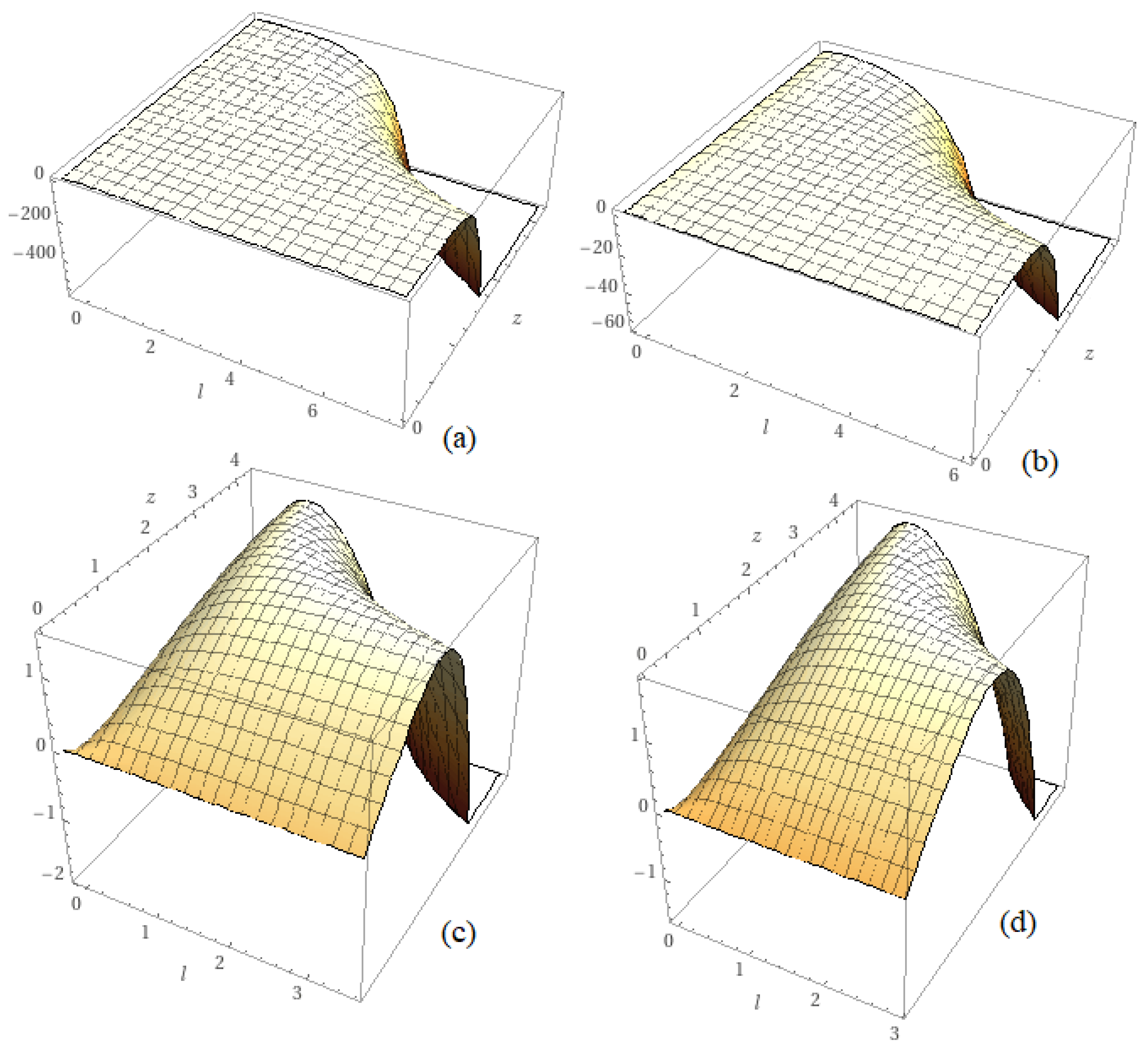
  • The above results are sharp such that the maximum function is given by the formula (see Figure 1)
    [ C Δ α , β , γ , κ , m h ( ξ ) ] q = ξ ( 1 ϱ ) + 1 ϱ + 1 ξ + 1 .
  • Let
    C Δ α , β , γ , κ , m ( ξ ) : = ξ + n = + 1 [ Σ n ] q ξ n , ξ .
    If C Δ α , β , γ , κ , m ( ξ ) and h ( ξ ) are a convex of order ϱ, then C Δ α , β , γ , κ , m h ( ξ ) is convex of order ρ , where
    ρ : = ( + 1 ) ( + 2 2 ϱ ) ( + 1 ) 3 2 ( + 2 ) ϱ + ϱ 2 1 .
Proof. 
By the assumptions of the proposition, the convex function
h ( ξ ) = ξ n = + 1 h n ξ n , ξ , N .
satisfies the inequality
n = + 1 n ( n ϱ ) 1 ϱ h n [ Σ n ] q 1 .
In addition, in view of Lemma 2 [22], we have that [ C Δ α , β , γ , κ , m h ( ξ ) ] q is also convex of order ϱ . This completes the first part.
Now, the first part gives the following inequalities:
( + 1 ) + 1 ϱ 1 ϱ n = + 1 h n [ Σ n ] q n = + 1 n n ϱ 1 ϱ h n [ Σ n ] q 1 ,
which yields
n = + 1 h n [ Σ n ] q 1 ϱ ( + 1 ) + 1 ϱ .
Moreover, we have
n = + 1 n h n [ Σ n ] q 1 ϱ + 1 ϱ .
Consequently, we obtain the second part and third parts respectively. Clearly, the maximum sharp function is given by the formula
[ C Δ α , β , γ , κ , m h ( ξ ) ] q = ξ ( 1 ϱ ) + 1 ϱ + 1 ξ + 1 .
A convolution property implies that
C Δ α , β , γ , κ , m h ( ξ ) = C Δ α , β , γ , κ , m × h ( ξ ) ,
where C Δ α , β , γ , κ , m and h are convex of order ϱ . To show that C Δ α , β , γ , κ , m h ( ξ ) is convex of order ρ , we have to show that
n = + 1 n n ρ 1 ρ h n [ Σ n ] q 1 .
Since
n = + 1 n n ϱ 1 ϱ h n 1 , n = + 1 n n ϱ 1 ϱ [ Σ n ] q 1 ,
then by the Cauchy–Schwarz inequality, we obtain
n = + 1 n n ϱ 1 ϱ h n [ Σ n ] q 1 , h n [ Σ n ] q 1 ϱ n ( n ϱ ) .
However, 1 ϱ n ( n ϱ ) ( n ϱ ) ( 1 ρ ) n ( 1 ϱ ) ( n ρ ) ; thus, a computation yields
ρ : = ( + 1 ) ( + 2 2 ϱ ) ( + 1 ) 3 2 ( + 2 ) ϱ + ϱ 2 1 .
Hence, in view of Lemma 2 [22], C Δ α , β , γ , κ , m h ( ξ ) is convex of order ρ . This completes the last part of the result.
Proposition 3.
Let h be starlike of order ϱ , ϱ [ 0 , 1 ) with non-positive coefficients ( h n 0 ). Moreover, let
n = + 1 n ϱ 1 ϱ h n [ Σ n ] q 1 .
Then,
  • [ C Δ α , β , γ , κ , m h ( ξ ) ] q is also starlike of order ϱ.
  • It achieves the next upper and lower bounds
    | ξ | 1 ϱ + 1 ϱ | ξ | + 1 | [ C Δ α , β , γ , κ , m h ( ξ ) ] q | | ξ | + 1 ϱ + 1 ϱ | ξ | + 1
  • and its derivative achieves the next upper and lower bounds
    1 ( 1 ϱ ) ( + 1 ) ( + 1 ϱ ) | ξ | | [ C Δ α , β , γ , κ , m h ( ξ ) ] q | 1 + ( 1 ϱ ) ( + 1 ) ( + 1 ϱ ) | ξ | .
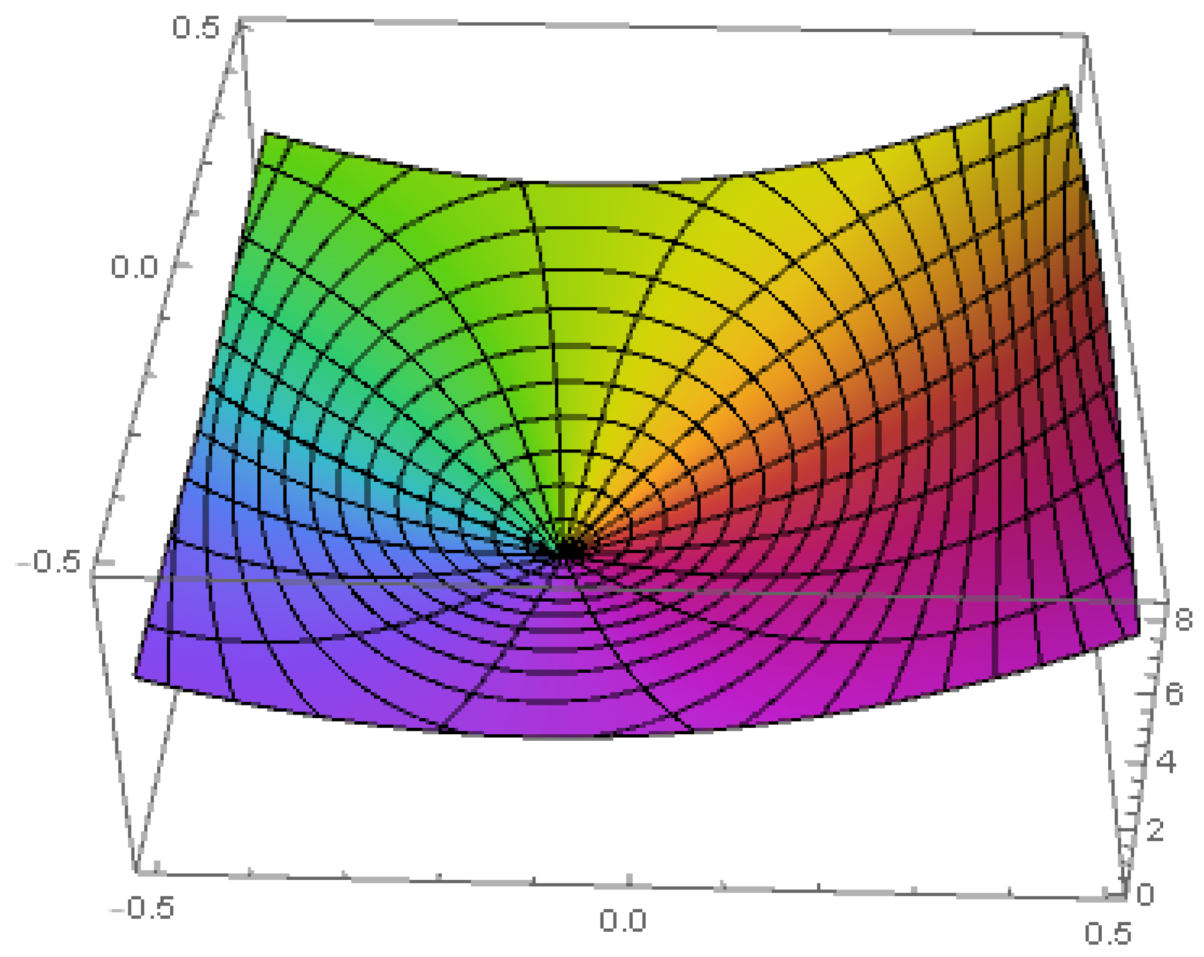
  • The above results are sharp such that the maximum function is given by the formula (see Figure 2)
    [ C Δ α , β , γ , κ , m h ( ξ ) ] q = ξ 1 ϱ + 1 ϱ ξ + 1 .
  • If C Δ α , β , γ , κ , m ( ξ ) and h ( ξ ) are starlike of order ϱ then C Δ α , β , γ , κ , m h ( ξ ) is starlike of order ρ , where
    ρ : = + 1 ϱ 2 + 2 2 ϱ .
Proof. 
Since h has non-positive coefficients, then it can be written as follows:
h ( ξ ) = ξ n = + 1 h n ξ n , ξ , N .
Moreover, since h is starlike of order ϱ , where ϱ [ 0 , 1 ) , satisfies the inequality
n = + 1 n ϱ 1 ϱ h n [ Σ n ] q 1 ,
then in view of Lemma 1 [22], we have [ C Δ α , β , γ , κ , m h ( ξ ) ] q is also starlike of order ϱ . This completes the first part.
By the first part of this result, we obtain
+ 1 ϱ 1 ϱ n = + 1 h n [ Σ n ] q n = + 1 n ϱ 1 ϱ h n [ Σ n ] q 1 ,
which yields
n = + 1 h n [ Σ n ] q 1 ϱ + 1 ϱ .
Consequently, we have
| [ C Δ α , β , γ , κ , m h ( ξ ) ] q | | ξ | | ξ | + 1 n = + 1 h n [ Σ n ] q | ξ | | ξ | + 1 1 ϱ + 1 ϱ
and
| [ C Δ α , β , γ , κ , m h ( ξ ) ] q | | ξ | + | ξ | + 1 n = + 1 h n [ Σ n ] q | ξ | + | ξ | + 1 1 ϱ + 1 ϱ .
Combining the above two inequalities, we obtain the second part. By using the fact,
n = + 1 n h n [ Σ n ] q 1 ϱ + ϱ ( 1 ϱ ) + 1 ϱ = ( + 1 ) ( 1 ϱ ) + 1 ϱ .
Therefore, a computation implies that
| [ C Δ α , β , γ , κ , m h ( ξ ) ] q | 1 | ξ | n = + 1 n h n [ Σ n ] q 1 ( 1 ϱ ) ( + 1 ) ( + 1 ϱ ) | ξ |
and
| [ C Δ α , β , γ , κ , m h ( ξ ) ] q | 1 + | ξ | n = + 1 n h n [ Σ n ] q 1 + ( 1 ϱ ) ( + 1 ) ( + 1 ϱ ) | ξ | .
Combining the above inequalities, we receive the third item. A direct calculation yields the maximum function placed as follows:
[ C Δ α , β , γ , κ , m h ( ξ ) ] q = ξ 1 ϱ + 1 ϱ ξ + 1 ,
which completes part four.
By the convolution definition, we have
C Δ α , β , γ , κ , m h ( ξ ) = C Δ α , β , γ , κ , m × h ( ξ ) ,
where C Δ α , β , γ , κ , m and h are starlike of order ϱ . To show that C Δ α , β , γ , κ , m h ( ξ ) is starlike of order ρ , we need to show that
n = + 1 n ρ 1 ρ h n [ Σ n ] q 1 .
Since
n = + 1 n ϱ 1 ϱ h n 1
and
n = + 1 n ϱ 1 ϱ [ Σ n ] q 1 ,
then in view of the Cauchy–Schwarz inequality, we obtain
n = + 1 n ϱ 1 ϱ h n [ Σ n ] q 1 ,
where
h n [ Σ n ] q 1 ϱ n ϱ .
However,
1 ϱ n ϱ ( n ϱ ) ( 1 ρ ) ( 1 ϱ ) ( n ρ ) ;
thus, the equality of the above conclusion yields
ρ : = + 1 ϱ 2 + 2 2 ϱ .
Hence, in view of Lemma 1 [22], C Δ α , β , γ , κ , m h ( ξ ) is starlike of order ρ . This completes the last part of the result. □
Note that the sufficient condition for convexity is
1 + ξ h ( ξ ) h ( ξ ) > 0
and the class of all these functions is denoted by C . Moreover, the sufficient condition for the starlikeness is
ξ h ( ξ ) h ( ξ ) > 0
and the class of all these functions is denoted by S * .
Combining the two definitions to obtain the following functional using the q–operator:
Definition 1.
Let h Λ . Define a functional [ ϵ J α , β , γ , κ , m h ( ξ ) ] q as follows:
[ ϵ J α , β , γ , κ , m h ( ξ ) ] q = ( 1 ϵ ) ξ [ C Δ α , β , γ , κ , m h ( ξ ) ] q [ C Δ α , β , γ , κ , m h ( ξ ) ] q + ϵ 1 + ξ [ C Δ α , β , γ , κ , m h ( ξ ) ] q [ C Δ α , β , γ , κ , m h ( ξ ) ] q .
The Formula (12) is a generalization of the functional appearing in [23]—P250 for a special type of convex integral operator. We advance to investigate extra properties utilizing the [ C Δ α , β , γ , κ , m ] q .

4. Differential Inequalities

We consider the following results ([23]—P258–P266).
Lemma 1.
Define the following set for a positive integer ,
H [ 1 , ] = { : ( ξ ) = 1 + h ξ + h + 1 ξ + 1 + } .
In addition, for > 0 , ( 1 , 1 ] , the function F H [ 1 , ] achieves
G ( ξ ) 1 + ( + ) ξ 1 ξ + ξ 1 + ξ g ( ξ ) .
If g H [ 1 , ] is a solution of the differential equation
ξ g ( ξ ) + G ( ξ ) .   g ( ξ ) = 1 ,
then
g ( ξ ) 1 ξ 1 + ξ , ξ ,
where ≺ indicates the subordination notion.
Lemma 2.
Let ϕ Λ . In addition, let λ > 0 and ς [ 0 , 1 ) . If one of the following inequalities
ξ ϕ ( ξ ) ϕ ( ξ ) 1 + ( 1 2 ς + λ ) ξ 1 ξ + λ ( 1 2 ς ) ξ 1 + ( 1 2 ς ) ξ g ( ξ ) ,
( 1 λ ) ξ ϕ ( ξ ) ϕ ( ξ ) + λ 1 + ξ ϕ ( ξ ) ϕ ( ξ ) 1 + ( 1 2 ς + λ ) ξ 1 ξ + λ ( 1 2 ς ) ξ 1 + ( 1 2 ς ) ξ g ( ξ ) ,
holds, then the λ —convex operator that acts on ϕ
Φ λ ( ξ ) = 1 λ 0 ξ ϕ 1 / λ ( τ ) τ 1 d τ λ
is starlike of order ς.
The main outcomes of this investigation are as follows:
Theorem 1.
Consider the functional in (12). If
[ ϵ J α , β , γ , κ , m h ( ξ ) ] q ( ξ ) , ξ ,
where
( ξ ) = exp 0 ξ [ ϵ J α , β , γ , κ , m h ( ξ ) ] q τ d τ 0 ξ exp 0 ζ [ ϵ J α , β , γ , κ , m h ( ξ ) ] q τ d τ ζ d ζ + 1 = 1 + n = 1 + n ξ n
satisfies
| n | 2 + + ( 1 ) n + 1 , N , n 1 ;
then,
[ ϵ J α , β , γ , κ , m h ( ξ ) ] q 1 ξ 1 + ξ , ξ .
Proof. 
Our aim is to apply Lemma 1. Clearly, [ ϵ J α , β , γ , κ , m h ( ξ ) ] q H [ 1 , ] , where [ ϵ J α , β , γ , κ , m ( 0 ) ] q = 1 . Formulate a function as follows:
g ( ξ ) = 1 + 2 ( + 1 ) ξ + ξ 2 1 ξ 2 = 1 + 2 ( + 1 ) ξ + 2 ξ 2 + 2 ( + 1 ) ξ 3 + 2 ξ 4 + 2 ( + 1 ) ξ 5 + O ( ξ 6 ) = 1 + n = + 1 ( 2 + + ( 1 ) n + 1 ) ξ n .
Obviously, g ( ξ ) is convex univalent in ∇ achieving (see Figure 3)
1 + ξ g ( ξ ) g ( ξ ) = 1 + 4 ξ ( ξ ( ( ξ 2 + 3 ) + ξ ( ξ + 3 ) + 3 ) + 1 ) ) ( 1 ξ 2 ) 3 2 ( ( ξ 2 + 1 ) + ( ξ + 1 ) 2 ) ( 1 ξ 2 ) 2 > 0
for all | ξ | < 1 and > 0 . Obviously, ( ξ ) is a solution of the differential equation
ξ ( ξ ) + G ( ξ ) .   ( ξ ) = 1 ,
where G ( ξ ) = [ ϵ J α , β , γ , κ , m h ( ξ ) ] q . Since
( ξ ) = 1 + n = + 1 n ξ n
achieves
| n | 2 + + ( 1 ) n + 1 , N ,
then we obtain the following inequality:
( ξ ) g ( ξ ) , ξ ,
where ≪ indicates the majority relation. Then, by [24]—Corollary 1 and for | ξ | ( 0.28 , 2 1 ) , we have
( ξ ) g ( ξ ) , ξ .
By the concept of the subordination, there occurs a function w ( ξ ) ,   | w ( ξ ) | | ξ | < 1 ,   w ( 0 ) = 0 then this implies that
( ξ ) = g ( w ( ξ ) ) , ξ .
By letting w ( ξ ) = ξ , we obtain
[ ϵ J α , β , γ , κ , m h ( ξ ) ] q g ( ξ ) , ξ ,
where
g ( ξ ) = 1 + 2 ( + 1 ) ξ + ξ 2 1 ξ 2 = 1 + ( 1 + ) ξ 1 ξ + ξ 1 + ξ .
Thus, by letting = = 1 in Lemma 1, we confirm that
f ( ξ ) 1 ξ 1 + ξ ,
which leads to the double inequality
[ ϵ J α , β , γ , κ , m h ( ξ ) ] q g ( ξ ) 1 ξ 1 + ξ .
Hence, we reach the fact
[ ϵ J α , β , γ , κ , m h ( ξ ) ] q 1 ξ 1 + ξ , ξ .
Theorem 2.
Consider the functional in (12). If
[ λ J α , β , γ , κ , m h ( ξ ) ] q λ ( ξ ) , ξ , λ > 0 ,
where
λ ( ξ ) = exp 0 ξ [ λ J α , β , γ , κ , m h ( ξ ) ] q λ τ d τ 0 ξ exp 0 ζ [ λ J α , β , γ , κ , m h ( ξ ) ] q λ τ d τ λ ζ d ζ + 1 = 1 + n = 1 + n ( λ ) ξ n
achieves
| n ( λ ) | | 2 ( 1 ) n 1 λ | , N , n 1 ,
then the λ —convex operator that acts on the q-operator [ C Δ α , β , γ , κ , m h ( ξ ) ] q ,
Φ λ ( ξ ) = 1 λ 0 ξ [ C Δ α , β , γ , κ , m h ( ξ ) ] q 1 / λ τ 1 d τ λ
is starlike in .
Proof. 
Our proof is based on Lemma 2. Eventually, [ λ J α , β , γ , κ , m h ( ξ ) ] q H [ 1 , ] , where [ λ J α , β , γ , κ , m ( 0 ) ] q = 1 . Formulate a function as follows:
g ( ξ ) = 1 + 2 ( λ + 1 ) ξ + ξ 2 1 ξ 2 = 1 + 2 ( λ + 1 ) ξ + 2 ξ 2 + 2 ( λ + 1 ) ξ 3 + 2 ξ 4 + 2 ( λ + 1 ) ξ 5 + O ( ξ 6 ) = 1 + n = + 1 ( 2 ( ( 1 ) n 1 ) λ ) ξ n .
Obviously, g ( ξ ) is convex univalent in ∇ satisfying
1 + ξ g ( ξ ) g ( ξ ) = 1 + 4 ξ ( ξ ( λ ( ξ 2 + 3 ) + ξ ( ξ + 3 ) + 3 ) + 1 ) ) ( 1 ξ 2 ) 3 2 ( λ ( ξ 2 + 1 ) + ( ξ + 1 ) 2 ) ( 1 ξ 2 ) 2 > 0
for all | ξ | < 1 , λ > 0 and > 0 . Clearly, λ ( ξ ) is a solution of the differential equation
λ ξ λ ( ξ ) + G ( ξ ) .   λ ( ξ ) = 1 ,
where G ( ξ ) = [ λ J α , β , γ , κ , m h ( ξ ) ] q . However,
λ ( ξ ) = 1 + n = + 1 n ( λ ) ξ n
satisfies
| n ( λ ) | | 2 ( ( 1 ) n 1 ) λ | , λ > 0 , N ,
then we conclude that
λ ( ξ ) g ( ξ ) , ξ .
Then, by [24]—Corollary 1 and for | ξ | ( 0.28 , 2 1 ) , we have
λ ( ξ ) g ( ξ ) , ξ .
Again the subordination definition implies that a function occurs with u ( ξ ) ,   | u ( ξ ) | | ξ | < 1 ,   u ( 0 ) = 0 such that
λ ( ξ ) = g ( u ( ξ ) ) , ξ .
By letting u ( ξ ) = ξ , we have
[ λ J α , β , γ , κ , m h ( ξ ) ] q g ( ξ ) , ξ ,
where
[ λ J α , β , γ , κ , m h ( ξ ) ] q = ( 1 λ ) ξ [ C Δ α , β , γ , κ , m h ( ξ ) ] q [ C Δ α , β , γ , κ , m h ( ξ ) ] q + λ 1 + ξ [ C Δ α , β , γ , κ , m h ( ξ ) ] q [ C Δ α , β , γ , κ , m h ( ξ ) ] q
and
g ( ξ ) = 1 + 2 ( λ + 1 ) ξ + ξ 2 1 ξ 2 = 1 + ( 1 + λ ) ξ 1 ξ + λ ξ 1 + ξ .
Thus, by considering ς = 0 in Lemma 2, we attain that the λ —convex operator that acts on the q-operator [ C Δ α , β , γ , κ , m h ( ξ ) ] q ,
Φ λ ( ξ ) = 1 λ 0 ξ [ C Δ α , β , γ , κ , m h ( ξ ) ] q 1 / λ τ 1 d τ λ , λ > 0 ,
is starlike in .
Theorem 3.
Consider the operator [ C Δ α , β , γ , κ , m h ( ξ ) ] q . Then,
[ C Δ α , β , γ , κ , m h ( ξ ) ] q S * ξ ν 1 0 ξ [ C Δ α , β , γ , κ , m h ( τ ) ] q τ ρ 1 k ( τ ) τ ρ 2 d τ 1 / ν S * ( 2 ν 1 2 ν ) ,
where k is convex univalent function, ν > 1 / 2 and ρ 1 0 , ρ 2 > 0 .
Moreover, if
k ( ξ ) = ξ 1 ξ , ρ 2 = 1 ,
then
[ C Δ α , β , γ , κ , m h ( ξ ) ] q S * ξ ν 1 0 ξ [ C Δ α , β , γ , κ , m h ( τ ) ] q τ ( 1 τ ) 1 / ρ 1 ρ 1 d τ 1 / ν S * ( 2 ν 1 2 ν ) ,
where k is convex univalent function and ρ 1 0 , ρ 2 > 0 .
Proof. 
Let k ( ξ ) = ξ + n = + 1 k n ξ n . First, we must show that
ξ ν 1 0 ξ [ C Δ α , β , γ , κ , m h ( τ ) ] q τ ρ 1 k ( τ ) τ ρ 2 d τ 1 / ν Λ .
By the definition of [ C Δ α , β , γ , κ , m h ( τ ) ] q , we have
I [ F , G ] ( ξ ) : = ξ ν 1 0 ξ [ C Δ α , β , γ , κ , m h ( τ ) ] q τ ρ 1 k ( τ ) τ ρ 2 d τ 1 / ν = ξ ν 1 0 ξ τ + n = + 1 h n Σ n τ n τ ρ 1 τ + n = + 1 k n τ n τ ρ 2 d τ 1 / ν = ξ ν 1 0 ξ 1 + n = + 1 h n Σ n τ n 1 ρ 1 1 + n = + 1 k n τ n 1 ρ 2 d τ 1 / ν = ξ ν 1 0 ξ 1 + ρ 1 n = + 1 h n Σ n τ n 1 + 1 + ρ 2 n = + 1 k n τ n 1 + d τ 1 / ν = ξ ν 1 0 ξ 1 + ρ 1 n = + 1 h n Σ n τ n 1 + d τ 1 / ν .
A direct integration yields the conclusion in (13). Since k ( ξ ) is convex in ∇, then it belongs to S * ( 1 / 2 ) (the class of starlike functions of order 1 / 2 ). However, the multiplication of starlike functions is also starlike; then, the integral I [ F , G ] ( ξ ) is starlike of order ( 2 ν 1 ) / 2 ν (see [23]—P169). The second part comes from the first part, when k ( ξ ) = ξ / ( 1 ξ ) and ρ 2 = 1 . Hence, the proof. □
Example 1.
Consider the differential equation
ξ [ C Δ α , β , γ , κ , m h ( ξ ) ] q [ C Δ α , β , γ , κ , m h ( ξ ) ] q = 1 ξ 1 + ξ ,
and the solution is given by
[ C Δ α , β , γ , κ , m h ( ξ ) ] q = ξ 1 ξ 2 ,
which is starlike (see Figure 1), and hence, in view of Theorem 3, we have
ξ ν 1 0 ξ [ C Δ α , β , γ , κ , m h ( τ ) ] q τ ( 1 τ ) 1 / ρ 1 ρ 1 d τ 1 / ν S * ( 2 ν 1 2 ν ) ,
where ρ 1 0 .
Example 2.
Consider the differential equation
ξ [ C Δ α , β , γ , κ , m h ( ξ ) ] q [ C Δ α , β , γ , κ , m h ( ξ ) ] q = 1 ,
and the outcome of the above equation is formulated by
[ C Δ α , β , γ , κ , m h ( ξ ) ] q = ξ ,
which satisfies
ξ [ C Δ α , β , γ , κ , m h ( ξ ) ] q [ C Δ α , β , γ , κ , m h ( ξ ) ] q = 1 > 0 ;
thus, it is starlike. According to Theorem 3, we have
ξ ν 1 0 ξ 1 ( 1 τ ) 1 / ρ 1 ρ 1 d τ 1 / ν S * ( 2 ν 1 2 ν ) ,
where ρ 1 0 .

5. Conclusions

From above, we conclude that the q–Prabhakar fractional differential operator of a complex variable can be studied in view of the geometric function theory by consuming a special class of analytic functions. Various differential inequalities are studied by the suggested operator and then its properties are investigated based on the concepts of subordination and superordination. A starlikeness of the operator implies a starlikeness of an integral formula, which indicates a solution of the well-known Briot–Bouquet differential equation (see Theorem 3). Finally, we presented the sharpness of convexity and starlikeness and estimate the corresponding extreme functions.
For future works, one can suggest the double QFC. Additionally, it is possible to extend the q–calculus to post quantum calculus, which is represented by the ( p , q )-calculus. In reality, such a QFC extension cannot be achieved by simply replacing q in the q-calculus with q / p . When p = 1 in the ( p , q )–calculus, one can derive the q-calculus. The number of double QFC is determined by
[ n ] p , q = p n q n p q .
Moreover, the double QFC derivative is given by
Δ p , q h ( ξ ) = h ( p ξ ) h ( q ξ ) ξ ( p q ) , 0 < q < p 1 , Δ p , q h ( 0 ) = h ( 0 ) .

Author Contributions

Conceptualization, R.W.I. and N.M.A.; methodology, R.W.I. and N.M.A.; formal analysis, R.W.I.; inquiry, R.W.I. and N.M.A.; and financing acquisition, N.M.A. All authors have read and agreed to the published version of the manuscript.

Funding

This research received no external funding.

Institutional Review Board Statement

Not applicable.

Informed Consent Statement

Not applicable.

Data Availability Statement

In this investigation, no recorded data were collected or examined. This article does not allow for the exchange of data.

Conflicts of Interest

The authors declare no conflict of interest.

References

  1. Jackson, F.H. q-form of Taylor’s theorem. Messenger Math. 1909, 38, 62–64. [Google Scholar]
  2. Exton, H. Q-Hypergeometric Functions and Applications; John Wiley & Sons, Inc.: New York, NY, USA, 1983; Volume 355. [Google Scholar]
  3. Celeghini, E.; Demartino, S.; Desiena, S.; Rasetti, M.; Vitiello, G. Quantum groups, coherent states, squeezing and lattice quantum mechanics. Ann. Phys. 1995, 241, 50–67. [Google Scholar] [CrossRef]
  4. Biedenharn, L.C. The quantum group SUq (2) and a q-analogue of the boson operators. J. Phys. A Math. Gen. 1989, 22, L873. [Google Scholar] [CrossRef]
  5. Ohnuki, Y.; Susumu, K. Quantum Field Theory and Parastatistics; University of Tokyo Press: Tokyo, Japan, 1982; pp. 100–110. [Google Scholar]
  6. Zirar, H. Some applications of fractional calculus operators to a certain subclass of analytic functions defined by integral operator involving generalized Hypergeometric function. Gen. Math. Notes 2016, 35, 19–35. [Google Scholar]
  7. Hadid, S.B.; Ibrahim, R.W.; Shaher, M. Multivalent functions and differential operator extended by the quantum calculus. Fractal Fract. 2022, 6, 354. [Google Scholar] [CrossRef]
  8. Arfaoui, S.; Maryam, G.A.; Ben, M.A. Quantum wavelet uncertainty principle. Fractal Fract. 2021, 6, 8. [Google Scholar] [CrossRef]
  9. Aldawish, I.; Ibrahim, R.W. Solvability of a new q-differential equation related to q-differential inequality of a special type of analytic functions. Fractal Fract. 2021, 5, 228. [Google Scholar] [CrossRef]
  10. Pishkoo, A.; Darus, M. On Meijer’s G-Functions (MGFs) and its applications. Rev. Theor. Sci. 2015, 3, 216–223. [Google Scholar] [CrossRef]
  11. Prabhakar, T.R. A singular integral equation with a generalized Mittag-Leffler function in the kernel. Yokohama Math. J. 1971, 19, 7–15. [Google Scholar]
  12. Garra, R.; Rudolf, G.; Federico, P.; Zivorad, T. Hilfer-Prabhakar derivatives and some applications. App. Math. Comp. 2014, 242, 576–589. [Google Scholar] [CrossRef]
  13. Garra, R.; Roberto, G. The Prabhakar or three parameter Mittag-Leffler function: Theory and application. Commun. Nonlinear Sci. Numer. Simul. 2018, 56, 314–329. [Google Scholar] [CrossRef]
  14. Giusti, A.; Ivano, C. Prabhakar-like fractional viscoelasticity. Commun. Nonlinear Sci. Numer. Simul. 2018, 56, 138–143. [Google Scholar] [CrossRef]
  15. Derakhshan, M.H. New numerical algorithm to solve variable-order fractional integrodifferential equations in the sense of Hilfer-Prabhakar derivative. Abstr. Appl. Anal. 2021, 2021, 1–10. [Google Scholar] [CrossRef]
  16. Eshaghi, S.; Alireza, A.; Reza, K.G. Generalized Mittag-Leffler stability of nonlinear fractional regularized Prabhakar differential systems. Int. J. Nonlinear Anal. Appl. 2021, 12, 665–678. [Google Scholar]
  17. Eghbali, N.; Aram, M.; Rassias, J. Mittag-Leffler-Hyers-Ulam stability of Prabhakar fractional integral equation. Int. J. Nonlinear Anal. Appl. 2021, 12, 25–33. [Google Scholar]
  18. Michelitsch, T.M.; Federico, P.; Alejandro, P.R. On discrete time Prabhakar-generalized fractional Poisson processes and related stochastic dynamics. Phys. A Stat. Mech. Appl. 2021, 565, 125541. [Google Scholar] [CrossRef]
  19. Kilbas, A.A.; Megumi, S.; Saxena, R.K. Generalized Mittag-Leffler function and generalized fractional calculus operators. Integral Transform. Spec. Funct. 2004, 15, 31–49. [Google Scholar] [CrossRef]
  20. Chen, M.P. On a class of starlike functions. Nanta Math. 1975, 8, 79–82. [Google Scholar]
  21. Sharma, S.K.; Jain, R. On some properties of generalized q-Mittag Leffler function. Math. Aeterna 2014, 4, 613–619. [Google Scholar]
  22. Srivastava, H.M.; Owa, S.; Chatterjea, S.K. A note on certain classes of starlike functions. Rend. Semin. Mat. Univ. Padova 1987, 77, 115–124. [Google Scholar]
  23. Miller, S.S.; Mocanu, P.T. Differential Subordinations. In Theory and Applications; Marcel Dekker Inc.: New York, NY, USA; Basel, Switzerland, 2000. [Google Scholar]
  24. Campbell, D.M. Majorization-subordination theorems for locally univalent functions, II. Canad. J. Math. 1973, 25, 420–425. [Google Scholar] [CrossRef]
Figure 1. 3D–plot of the maximum function of convexity for ϱ , (a):0; (b):0.25; (c):0.5; (d): 0.6.
Fractalfract 06 00545 g001
Figure 2. 3D–Plot of the maximum function of starlikeness for ϱ = 0.5 .
Fractalfract 06 00545 g002
Figure 3. The plot of the convex function g ( ξ ) , = 1 , λ = 0.5 .
Fractalfract 06 00545 g003
Publisher’s Note: MDPI stays neutral with regard to jurisdictional claims in published maps and institutional affiliations.

