Article

Fractal–Fractional Michaelis–Menten Enzymatic Reaction Model via Different Kernels

1
Department of Mathematics, College of Sciences and Arts, Najran University, Najran P.O. Box 1988, Saudi Arabia
2
Department of Mathematics, Faculty of Applied Science, Taiz University, Taiz P.O. Box 6803, Yemen
*
Author to whom correspondence should be addressed.
Fractal Fract. 2022, 6(1), 13; https://doi.org/10.3390/fractalfract6010013
Submission received: 14 November 2021 / Revised: 19 December 2021 / Accepted: 23 December 2021 / Published: 29 December 2021

Abstract

:
In this paper, three new models of fractal–fractional Michaelis–Menten enzymatic reaction (FFMMER) are studied. We present these models based on three different kernels, namely, power law, exponential decay, and Mittag-Leffler kernels. We construct three schema of successive approximations according to the theory of fractional calculus and with the help of Lagrange polynomials. The approximate solutions are compared with the resulting numerical solutions using the finite difference method (FDM). Because the approximate solutions in the classical case of the three models are very close to each other and almost matches, it is sufficient to compare one model, and the results were good. We investigate the effects of the fractal order and fractional order for all models. All calculations were performed using Mathematica software.

1. Introduction

Shateyi et al. [1] proposed a method which is an extension of the spectral homotopy analysis method for investigating the approximate solution of the Michaelis–Menten enzymatic reaction equation. They compared the results of Runge–Kutta routines for measuring the accuracy and efficiency. Abu-Reesh [2] derived analytical equations for the optimal design of a number of membrane reactors in series performing enzyme catalyzed reactions. This enzyme is described by Michaelis–Menten kinetics with competitive product inhibition. In terms of the Lambert W ( x ) function, Golicnik [3] proposed an exact closed-form solution to the Michaelis–Menten equation. Golicnik [4] showed that analysis of the progress-curve data can be carried out through explicit mathematical equations; this analysis can be performed using any nonlinear regression-curve fitting program. In addition, he found that when the progress curves are analyzed by the direct solution of the integrated Michaelis–Menten equation, there were three different demonstrated approximations of W ( x ) with relatively high accuracy that are appropriate to utilize. In many studies, they studied this system and proposed many different kinds of approximate analytical solutions [5,6,7,8,9]. Hussam et al. [10] investigated the semianalytical results of fractional time enzyme kinetics using the Laplace transformation and Adomian decomposition method. In general, due to the difficulty that many researchers face in finding exact solutions to fractional differential equations, many researchers have presented numerical, approximate methods and applications to treat this problem (see [11,12,13,14,15,16,17,18,19,20,21,22]). In fact, there are no other methods that deal with numerical solutions in the fractal–fractional sense, except [23].
In [24], the authors investigated spectral methods in the sense of fractal–fractional differentiation. However, it included only the studies using Mittag-Leffler kernel. The importance of our study lies here, as we provide a treatment for more than one kernel and for a longer time. Many of the previous studies deal with approximate solutions in the case of a short time. Our work, along with some of the previous studies in the sense of fractal–fractional differentiation, contributes to providing numerical algorithms that researchers can apply to many models related to the real world.
This paper focuses on presenting the classical model in the form of three fractal–fractional models with different kernels. These treatments will be carried out based on the primary sources [23] as well as similar treatments that were carried out by many authors (see [25,26,27]). Atangana [23] proposed new operators of differentiation as convolution of power law, exponential decay law, and generalized Mittag-Leffler law with fractal derivatives. These operators are referred to as fractal–fractional differential and integral operators.
To this end [23], we replace the derivative with respect to t by the fractal–fractional derivatives power (FFP) law, the fractal–fractional exponential (FFE), and the fractal–fractional Mittag-Leffler (FFM) kernels in sense of Riemann–Liouville which correspond to the Caputo [28], Caputo–Fabrizio (CF) [29], and the Atangana–Baleanu (AB) [30] fractional derivatives, respectively.
Michaelis and Menten show that the rate of an enzyme-catalyzed reaction is proportional to the concentration of the enzyme–substrate complex predicted by the Michaelis–Menten equations [31]. The dynamic form of this model [31] is given by
d α 1 d t = δ α 1 ( t ) β 1 ( t ) + γ α 2 ( t ) ,
d β 1 d t = δ α 1 ( t ) β 1 ( t ) + ( γ + σ ) α 2 ( t ) ,
d α 2 d t = δ α 1 ( t ) β 1 ( t ) ( γ + σ ) α 2 ( t ) ,
d β 2 d t = σ α 2 ( t ) ,
α 1 ( t ) is the concentration of a substrate, β 1 ( t ) is the concentration of an enzyme, α 2 ( t ) is the concentration of the resulting complex, and β 2 ( t ) is the concentration of the resulting product. δ , γ , and σ represent the rate of reaction governing the production of the complex from the α 1 ( t ) and the β 1 ( t ) , the rate of reaction governing decomposition of the complex to the β 1 ( t ) and the β 1 ( t ) , and the rate of reaction governing the breakdown of the complex into the β 2 ( t ) and the β 1 ( t ) . In addition, the initial conditions are α 1 ( 0 ) = α 10 , β 1 ( 0 ) = β 10 , α 2 ( 0 ) = α 20 , and β 2 ( 0 ) = β 20 .
This model is used to study enzyme kinetic reactions, and the schematic is given by
α 1 + β 1 α 2 β 1 + β 2 .
Based on this schematic, a complex α 2 is the product of a reaction between a substrate α 1 and an enzyme β 1 . Finally, a complex α 2 is converted into a product β 2 and the enzyme β 1 .
To our best knowledge, this is the first study of this the fractal–fractional Michaelis–Menten enzymatic reaction using power, exponential decay, and Mittag-Leffler laws.
The paper is organized as follows. In Section 2, we give a background about the definitions of the fractal–fractional operators via the power, exponential decay, and Mittag-Leffler kernels. In addition we construct the successive iterations of the fractal–fractional Michaelis–Menten enzymatic reaction via three kernels. In Section 3, we present the numerical results. Finally, in Section 4 and Section 5, we explain and discuss the numerical results and give some concluding remarks.

2. Numerical Schemes of Fractal–Fractional Michaelis–Menten Enzymatic Reaction Model

In this section, we provide the necessary definitions for this work. For more details on these definitions, refer to references [23]. In addition, we present the construction of the numerical schemes of the Fractal–Fractional Michaelis–Menten enzymatic reaction model according to the power, exponential decay, and Mittag-Leffler laws. For the theoretical parts of these fractal–fractional operators due to the three different kernels, the reader should refer to [23].

2.1. Preliminaries and Notation

Definition 1.
If η ( t ) is continuous and fractal differentiable on ( a , b ) of order k, then the fractal–fractional derivative of η ( t ) of order ϱ in the Rieman–Liouville sense with the power law is given by [23]:
0 FFP D t ϱ ,   k η ( t ) = 1 Γ ( 1 ϱ ) d d t k 0 t ( t τ ) ϱ η ( τ ) d τ , ( 0 < ϱ ,   k 1 ) ,
and the fractal–fractional integral of η ( t ) is given by
0 FFP I t ϱ ,   k η ( t ) = k Γ ( ϱ ) 0 t τ k 1 ( t τ ) ϱ 1 η ( τ ) d τ .
Definition 2.
If η ( t ) is continuous in the ( a , b ) and fractal differentiable on ( a , b ) with order k, then the fractal–fractional derivative of η ( t ) of order ϱ in the Caputo–Fabrizio sense with the exponential decay kernel is given by [28]
0 FFE D t ϱ , k η ( t ) = M ( ϱ ) 1 ϱ d d t k 0 t e ϱ 1 ϱ ( t τ ) η ( τ ) d τ , ( 0 < ϱ ,   k 1 ) ,
and the fractal–fractional integral of η ( t ) is given by
0 FFE I t ϱ , k η ( t ) = ( 1 ϱ ) k t k 1 M ( ϱ ) η ( t ) + ϱ k M ( ϱ ) 0 t τ k 1 η ( τ ) d τ
where M ( ϱ ) is the normalization function such that M ( 0 ) = M ( 1 ) = 1 .
Definition 3.
If η ( t ) is continuous in the ( a , b ) and fractal differentiable on ( a , b ) with order k, then the fractal–fractional derivative of η ( t ) of order ϱ in the Atangana–Baleanu sense with the the Mittag-Leffler-type kernel is given by [23]
0 F F M D t ϱ , k η ( t ) = A ( ϱ ) 1 ϱ d d t k 0 t E ϱ ϱ 1 ϱ ( t τ ) η ( τ ) d τ , ( 0 < ϱ ,   k 1 ) ,
and the fractal–fractional integral of η ( t ) is given by
0 F F M I t ϱ , k η ( t ) = ( 1 ϱ ) k t k 1 A ( ϱ ) η ( t ) + ϱ   k A ( ϱ ) Γ ( ϱ ) 0 t τ k 1 ( t τ ) ϱ 1 η ( τ ) d τ ,
d η ( t ) d t k = l i m τ t η ( τ ) η ( t ) τ k t k
where A ( ϱ ) = 1 ϱ + ϱ Γ ( ϱ ) is a normalization function.

2.2. FFMMER Scheme via the Power-Law Kernel

In the present subsection, we apply the fractal–fractional operator with power-law kernel to the FFMMER described above. We follow the same procedure as in [23], and we have
0 FFP D t ϱ β 1 ( t ) = δ α 1 ( t ) β 1 ( t ) + γ α 2 ( t ) ,
0 FFP D t ϱ α 1 ( t ) = δ α 1 ( t ) β 1 ( t ) + ( γ + σ ) α 2 ( t ) ,
0 FFP D t ϱ β 2 ( t ) = δ α 1 ( t ) β 1 ( t ) ( γ + σ ) α 2 ( t ) ,
0 FFP D t ϱ α 2 ( t ) = σ α 2 ( t ) .
Following the same method as in [23], we have the successive approximations
α 1 ( t ) α 1 ( 0 ) = k Γ ( ϱ ) 0 t τ k 1 ( t τ ) ϱ 1 μ 1 ( α 1 , β 1 , α 2 , β 2 , τ ) d τ ,
β 1 ( t ) β 1 ( 0 ) = k Γ ( ϱ ) 0 t τ k 1 ( t τ ) ϱ 1 μ 2 ( α 1 , β 1 , α 2 , β 2 , τ ) d τ ,
α 2 ( t ) α 2 ( 0 ) = k Γ ( ϱ ) 0 t τ k 1 ( t τ ) ϱ 1 μ 3 ( α 1 , β 1 , α 2 , β 2 , τ ) d τ ,
β 2 ( t ) β 2 ( 0 ) = k Γ ( ϱ ) 0 t τ k 1 ( t η ) α 1 μ 4 ( α 1 , β 1 , α 2 , β 2 , τ ) d η
where
μ 1 ( α 1 , β 1 , α 2 , β 2 , τ ) = δ α 1 ( τ ) β 1 ( τ ) + γ α 2 ( τ ) ,
μ 2 ( α 1 , β 1 , α 2 , β 2 , τ ) = δ α 1 ( τ ) β 1 ( τ ) + ( γ + σ ) α 2 ( τ ) ,
μ 3 ( α 1 , β 1 , α 2 , β 2 , τ ) = δ α 1 ( τ ) β 1 ( τ ) ( γ + σ ) α 2 ( τ ) ,
μ 4 ( α 1 , β 1 , α 2 , β 2 , τ ) = σ α 2 ( τ ) .
Now, we can reformulate Equations (16)–(19) as
α 1 ( t ) α 1 ( 0 ) = k Γ ( ϱ ) m = 0 t m t m + 1 τ k 1 ( t m + 1 τ ) ϱ 1 μ 1 ( α 1 , β 1 , α 2 , β 2 , τ ) d τ ,
β 1 ( t ) β 1 ( 0 ) = k Γ ( ϱ ) m = 0 t m t m + 1 τ k 1 ( t m + 1 τ ) ϱ 1 μ 2 ( α 1 ( τ ) , β 1 ( τ ) , α 2 ( τ ) , β 2 ( τ ) , τ ) d τ ,
α 2 ( t ) α 2 ( 0 ) = k Γ ( ϱ ) m = 0 t m t m + 1 τ k 1 ( t m + 1 τ ) ϱ 1 μ 3 ( α 1 , β 1 , α 2 , β 2 , τ ) d τ ,
β 2 ( t ) β 2 ( 0 ) = k Γ ( ϱ ) m = 0 t m t m + 1 τ k 1 ( t m + 1 τ ) ϱ 1 μ 4 ( α 1 , β 1 , α 2 , β 2 , τ ) d τ .
When we use the two-step Lagrange polynomial interpolation, we can obtain
α 1 ( t ) α 1 ( 0 ) = k Γ ( ϱ ) m = 0 t m t m + 1 τ k 1 ( t m + 1 τ ) ϱ 1 Q 1 , m ( τ ) d τ ,
β 1 ( t ) β 1 ( 0 ) = k Γ ( ϱ ) m = 0 t m t m + 1 τ k 1 ( t m + 1 τ ) ϱ 1 Q 2 , m ( τ ) d τ ,
α 2 ( t ) α 2 ( 0 ) = k Γ ( ϱ ) m = 0 t m t m + 1 τ k 1 ( t m + 1 τ ) ϱ 1 Q 3 , m ( τ ) d τ ,
β 2 ( t ) β 2 ( 0 ) = k Γ ( ϱ ) m = 0 t m t m + 1 τ k 1 ( t m + 1 τ ) ϱ 1 Q 4 , m ( τ ) d τ ,
where,
Q 1 , m ( τ ) = τ t m 1 t m t m 1 t m k 1 μ 1 ( α 1 ( τ m ) , β 1 ( τ m ) , α 2 ( τ m ) , β 2 ( τ m ) , τ m ) τ t m t m t m 1 × t m 1 k 1 μ 1 ( α 1 ( τ m 1 ) , β 1 ( τ m 1 ) , α 2 ( τ m 1 ) , β 2 ( τ m 1 ) , τ m 1 ) ,
Q 2 , m ( τ ) = τ t m 1 t m t m 1 t m k 1 μ 2 ( α 1 ( τ m ) , β 1 ( τ m ) , α 2 ( τ m ) , β 2 ( τ m ) , τ m ) τ t m t m t m 1 × t m 1 k 1 μ 2 ( α 1 ( τ m 1 ) , β 1 ( τ m 1 ) , α 2 ( τ m 1 ) , β 2 ( τ m 1 ) , τ m 1 ) ,
Q 3 , m ( τ ) = τ t m 1 t m t m 1 t m k 1 μ 3 ( α 1 ( τ m ) , β 1 ( τ m ) , α 2 ( τ m ) , β 2 ( τ m ) , τ m ) τ t m t m t m 1 × t m 1 k 1 μ 3 ( α 1 ( τ m 1 ) , β 1 ( τ m 1 ) , α 2 ( τ m 1 ) , β 2 ( τ m 1 ) , τ m 1 ) ,
Q 4 , m ( τ ) = τ t m 1 t m t m 1 t m k 1 μ 4 ( η 4 ( τ m ) , β 1 ( τ m ) , α 2 ( τ m ) , β 2 ( τ m ) , τ m ) τ t m t m t m 1 × t m 1 k 1 μ 4 ( α 1 ( τ m 1 ) , β 1 ( τ m 1 ) , α 2 ( τ m 1 ) , β 2 ( τ m 1 ) , τ m 1 ) .
To obtain the numerical solutions of (12)–(15) involving the power-law kernel, we integrate Equations (28)–(31) directly
α 1 ( t n + 1 ) = α 1 ( 0 ) + k h ϱ Γ ( ϱ + 2 ) m = 0 n t m k 1 μ 1 ( α 1 ( t m ) , β 1 ( t m ) , α 2 ( t m ) , β 2 ( t m ) , t m ) Ξ 1 ( n , m ) t m 1 k 1 μ 1 ( α 1 ( τ m 1 ) , β 1 ( t m 1 ) , α 2 ( t m 1 ) , β 2 ( t m 1 ) , t m 1 ) Ξ 2 ( n , m ) ) ,
β 1 ( t n + 1 ) = β 1 ( 0 ) + k h ϱ Γ ( ϱ + 2 ) m = 0 n t m k 1 μ 2 ( α 1 ( t m ) , β 1 ( t m ) , α 2 ( t m ) , β 2 ( t m ) , t m ) Ξ 1 ( n , m ) t m 1 k 1 μ 2 ( α 1 ( τ m 1 ) , β 1 ( t m 1 ) , α 2 ( t m 1 ) , β 2 ( t m 1 ) , t m 1 ) Ξ 2 ( n , m ) ) ,
α 2 ( t n + 1 ) = α 2 ( 0 ) + k h ϱ Γ ( ϱ + 2 ) m = 0 n t m k 1 μ 3 ( α 1 ( t m ) , β 1 ( t m ) , α 2 ( t m ) , β 2 ( t m ) , t m ) Ξ 1 ( n , m ) t m 1 k 1 μ 4 ( α 1 ( τ m 1 ) , β 1 ( t m 1 ) , α 2 ( t m 1 ) , β 2 ( t m 1 ) , t m 1 ) Ξ 2 ( n , m ) ) ,
β 2 ( t n + 1 ) = β 2 ( 0 ) + k h ϱ Γ ( ϱ + 2 ) m = 0 n t m k 1 μ 4 ( α 1 ( t m ) , β 1 ( t m ) , α 2 ( t m ) , β 2 ( t m ) , t m ) Ξ 1 ( n , m ) t m 1 k 1 μ 4 ( α 1 ( τ m 1 ) , β 1 ( t m 1 ) , α 2 ( t m 1 ) , β 2 ( t m 1 ) , t m 1 ) Ξ 2 ( n , m ) ) ,
Ξ 1 ( n , m ) = ( n + 1 m ) ϱ ( n m + 2 + ϱ ) ( n m ) ϱ × ( n m + 2 + 2 ϱ ) ,
Ξ 2 ( n , m ) = ( n + 1 m ) ϱ + 1 ( n m ) ϱ ( n m + 1 + ϱ ) .

2.3. FFMMER Scheme via the Exponential Decay Kernel

In the present subsection, we consider the following fractal–fractional operator with the exponential decay kernel to the FFMMER described above.
0 FFE D t ϱ β 1 ( t ) = δ α 1 ( t ) β 1 ( t ) + γ α 2 ( t ) ,
0 FFE D t ϱ α 1 ( t ) = δ α 1 ( t ) β 1 ( t ) + ( γ + σ ) α 2 ( t ) ,
0 FFE D t ϱ β 2 ( t ) = δ α 1 ( t ) β 1 ( t ) ( γ + σ ) α 2 ( t ) ,
0 FFE D t ϱ α 2 ( t ) = σ α 2 ( t ) .
For the successive approximations of the system of Equations (42)–(45), we follow the same procedures as in [23], and obtain
α 1 ( t ) α 1 ( 0 ) = k t k 1 ( 1 ϱ ) M ( ϱ ) μ 1 ( α 1 , β 1 , α 2 , β 2 , t ) + ϱ M ( ϱ ) 0 t k   τ k 1 μ 1 ( α 1 , β 1 , α 2 , β 2 , τ ) d τ ,
β 1 ( t ) β 1 ( 0 ) = k t k 1 ( 1 ϱ ) M ( ϱ ) μ 2 ( α 1 , β 1 , α 2 , β 2 , t ) + ϱ M ( ϱ ) 0 t k   τ k 1 μ 2 ( α 1 , β 1 , α 2 , β 2 , τ ) d τ ,
α 2 ( t ) α 2 ( 0 ) = k t k 1 ( 1 ϱ ) M ( ϱ ) μ 3 ( α 1 , β 1 , α 2 , β 2 , t ) + ϱ M ( ϱ ) 0 t k   τ k 1 μ 3 ( α 1 , β 1 , α 2 , β 2 , τ ) d τ ,
β 2 ( t ) β 2 ( 0 ) = k t k 1 ( 1 ϱ ) M ( ϱ ) μ 4 ( α 1 , β 1 , α 2 , β 2 , t ) + ϱ M ( ϱ ) 0 t k   τ k 1 μ 4 ( α 1 , β 1 , α 2 , β 2 , τ ) d τ .
Using t = t n + 1 , the following is established:
α 1 ( t n + 1 ) α 1 ( t n ) = k t k 1 ( 1 ϱ ) M ( ϱ ) μ 1 ( α 1 , β 1 , α 2 , β 2 , t ) + ϱ M ( ϱ ) 0 t n + 1 k   τ k 1 μ 1 ( α 1 , β 1 , α 2 , β 2 , τ ) d τ ,
β 1 ( t n + 1 ) β 1 ( t n ) = k t k 1 ( 1 ϱ ) M ( ϱ ) μ 2 ( α 1 , β 1 , α 2 , β 2 , t ) + ϱ M ( ϱ ) 0 t n + 1 k   τ k 1 μ 2 ( α 1 , β 1 , α 2 , β 2 , τ ) d τ ,
α 2 ( t n + 1 ) α 2 ( t n ) = k t k 1 ( 1 ϱ ) M ( ϱ ) μ 3 ( α 1 , β 1 , α 2 , β 2 , t ) + ϱ M ( ϱ ) 0 t n + 1 k   τ k 1 μ 3 ( α 1 , β 1 , α 2 , β 2 , τ ) d τ ,
β 2 ( t n + 1 ) β 2 ( t n ) = k t k 1 ( 1 ϱ ) M ( ϱ ) μ 4 ( α 1 , β 1 , α 2 , β 2 , t ) + ϱ M ( ϱ ) 0 t n + 1 k   τ k 1 μ 4 ( α 1 , β 1 , α 2 , β 2 , τ ) d τ .
Further, we have the following:
α 1 ( t n + 1 ) α 1 ( t n ) = k t n k 1 ( 1 ϱ ) M ( ϱ ) μ 1 ( α 1 , β 1 , α 2 , β 2 , t n ) k t n 1 k 1 ( 1 ϱ ) M ( ϱ ) μ 1 ( α 1 , β 1 , α 2 , β 2 , t n 1 ) + ϱ M ( ϱ ) t n t n + 1 k   τ k 1 μ 1 ( α 1 , β 1 , α 2 , β 2 , τ ) d τ ,
β 1 ( t n + 1 ) β 1 ( t n ) = k t n k 1 ( 1 ϱ ) M ( ϱ ) μ 2 ( α 1 , β 1 , α 2 , β 2 , t n ) k t n 1 k 1 ( 1 ϱ ) M ( ϱ ) μ 2 ( α 1 , β 1 , α 2 , β 2 , t n 1 ) + ϱ M ( ϱ ) t n t n + 1 k   τ k 1 μ 2 ( α 1 , β 1 , α 2 , β 2 , τ ) d τ ,
α 2 ( t n + 1 ) α 2 ( t n ) = k t n k 1 ( 1 ϱ ) M ( ϱ ) μ 3 ( α 1 , β 1 , α 2 , β 2 , t n ) k t n 1 k 1 ( 1 ϱ ) M ( ϱ ) μ 3 ( α 1 , β 1 , α 2 , β 2 , t n 1 ) + ϱ M ( ϱ ) t n t n + 1 k   τ k 1 μ 3 ( α 1 , β 1 , α 2 , β 2 , τ ) d τ ,
β 2 ( t n + 1 ) β 2 ( t n ) = k t n k 1 ( 1 ϱ ) M ( ϱ ) μ 4 ( α 1 , β 1 , α 2 , β 2 , t n ) k t n 1 k 1 ( 1 ϱ ) M ( ϱ ) μ 4 ( α 1 , β 1 , α 2 , β 2 , t n 1 ) + ϱ M ( ϱ ) t n t n + 1 k   τ k 1 μ 4 ( α 1 , β 1 , α 2 , β 2 , τ ) d τ .
It follows from the Lagrange polynomial interpolation and integration of the following expressions:
α 1 ( t n + 1 ) α 1 ( t n ) = k t n k 1 ( 1 ϱ ) M ( ϱ ) μ 1 ( α 1 , β 1 , α 2 , β 2 , t n ) k t n 1 k 1 ( 1 ϱ ) M ( ϱ ) μ 1 ( α 1 , β 1 , α 2 , β 2 , t n 1 ) + k h ϱ 2 M ( ϱ ) × ( 3 t n k 1 μ 1 ( α 1 , β 1 , α 2 , β 2 , t n ) t n 1 k 1 μ 1 ( α 1 , β 1 , α 2 , β 2 , t n 1 ) ,
β 1 ( t n + 1 ) β 1 ( t n ) = k t n k 1 ( 1 ϱ ) M ( ϱ ) μ 2 ( α 1 , β 1 , α 2 , β 2 , t n ) k t n 1 k 1 ( 1 ϱ ) M ( ϱ ) μ 2 ( α 1 , β 1 , α 2 , β 2 , t n 1 ) + k h ϱ 2 M ( ϱ ) × ( 3 t n k 1 μ 2 ( α 1 , β 1 , α 2 , β 2 , t n ) t n 1 k 1 μ 2 ( α 1 , β 1 , α 2 , β 2 , t n 1 ) ,
α 2 ( t n + 1 ) α 2 ( t n ) = k t n k 1 ( 1 ϱ ) M ( ϱ ) μ 3 ( α 1 , β 1 , α 2 , β 2 , t n ) k t n 1 k 1 ( 1 ϱ ) M ( ϱ ) μ 3 ( α 1 , β 1 , α 2 , β 2 , t n 1 ) + k h ϱ 2 M ( ϱ ) × ( 3 t n k 1 μ 3 ( α 1 , β 1 , α 2 , β 2 , t n ) t n 1 k 1 μ 3 ( α 1 , β 1 , α 2 , β 2 , t n 1 ) ,
β 2 ( t n + 1 ) β 2 ( t n ) = k t n k 1 ( 1 ϱ ) M ( ϱ ) μ 4 ( α 1 , β 1 , α 2 , β 2 , t n ) k t n 1 k 1 ( 1 ϱ ) M ( ϱ ) μ 4 ( α 1 , β 1 , α 2 , β 2 , t n 1 ) + k h ϱ 2 M ( ϱ ) × ( 3 t n k 1 μ 4 ( α 1 , β 1 , α 2 , β 2 , t n ) t n 1 k 1 μ 4 ( α 1 , β 1 , α 2 , β 2 , t n 1 ) .
Finally, it is appropriate to write the successive approximations of the system Equations (42)–(45) as follows:
α 1 ( t n + 1 ) α 1 ( t n ) = k t n k 1 ( 1 ϱ ) M ( ϱ ) + 3 h ϱ 2 M μ 1 ( α 1 , β 1 , α 2 , β 2 , t n ) k t n 1 k 1 ( 1 ϱ ) M ( ϱ ) + h ϱ 2 M ( ϱ ) μ 1 ( α 1 , β 1 , α 2 , β 2 , t n 1 ) ,
β 1 ( t n + 1 ) β 1 ( t n ) = k t n k 1 ( 1 ϱ ) M ( ϱ ) + 3 h ϱ 2 M μ 2 ( α 1 , β 1 , α 2 , β 2 , t n ) k t n 1 k 1 ( 1 ϱ ) M ( ϱ ) + h ϱ 2 M ( ϱ ) μ 2 ( α 1 , β 1 , α 2 , β 2 , t n 1 ) ,
α 2 ( t n + 1 ) α 2 ( t n ) = k t n k 1 ( 1 ϱ ) M ( ϱ ) + 3 h ϱ 2 M μ 3 ( α 1 , β 1 , α 2 , β 2 , t n ) k t n 1 k 1 ( 1 ϱ ) M ( ϱ ) + h ϱ 2 M ( ϱ ) μ 3 ( α 1 , β 1 , α 2 , β 2 , t n 1 ) ,
β 2 ( t n + 1 ) β 2 ( t n ) = k t n k 1 ( 1 ϱ ) M ( ϱ ) + 3 h ϱ 2 M μ 4 ( α 1 , β 1 , α 2 , β 2 , t n ) k t n 1 k 1 ( 1 ϱ ) M ( ϱ ) + h ϱ 2 M ( ϱ ) μ 4 ( α 1 , β 1 , α 2 , β 2 , t n 1 ) .

2.4. FFMMER Scheme via the Mittag-Leffler Kernel

Finally, in this subsection, we consider FFMMER with the Mittag-Leffler kernel and, following the same procedure as in [23], we obtain
0 FFM D t ϱ α 1 ( t ) = δ α 1 ( t ) β 1 ( t ) + γ α 2 ( t ) ,
0 FFM D t ϱ β 1 ( t ) = δ α 1 ( t ) β 1 ( t ) + ( γ + σ ) α 2 ( t ) ,
0 FFM D t ϱ β 2 ( t ) = δ α 1 ( t ) β 1 ( t ) ( γ + σ ) α 2 ( t ) ,
0 FFM D t ϱ α 2 ( t ) = σ α 2 ( t ) .
We treat the following system Equations (66)–(69) based on Mittag-Leffler kernel as in [23], and we have
α 1 ( t ) α 1 ( 0 ) = k t k 1 ( 1 ϱ ) A ( ϱ ) μ 1 ( α 1 , β 1 , α 2 , β 2 , t ) + ϱ A ( ϱ ) Γ ( ϱ ) 0 t k   τ k 1 ( t τ ) ϱ 1 μ 1 ( α 1 , β 1 , α 2 , β 2 , τ ) d τ ,
β 1 ( t ) β 1 ( 0 ) = k t k 1 ( 1 ϱ ) A ( ϱ ) μ 2 ( α 1 , β 1 , α 2 , β 2 , t ) + ϱ A ( ϱ ) Γ ( ϱ ) 0 t k   τ k 1 ( t τ ) ϱ 1 μ 2 ( α 1 , β 1 , α 2 , β 2 , τ ) d τ ,
α 2 ( t ) α 2 ( 0 ) = k t k 1 ( 1 ϱ ) A ( ϱ ) μ 3 ( α 1 , β 1 , α 2 , β 2 , t ) + ϱ A ( ϱ ) Γ ( ϱ ) 0 t k   τ k 1 ( t τ ) ϱ 1 μ 3 ( α 1 , β 1 , α 2 , β 2 , τ ) d τ ,
β 2 ( t ) β 2 ( 0 ) = k t k 1 ( 1 ϱ ) A ( ϱ ) μ 4 ( α 1 , β 1 , α 2 , β 2 , t ) + ϱ A ( ϱ ) Γ ( ϱ ) 0 t k   τ k 1 ( t τ ) ϱ 1 μ 4 ( α 1 , β 1 , α 2 , β 2 , τ ) d τ .
When t n + 1 , we have the following:
α 1 ( t n + 1 ) α 1 ( 0 ) = k t n k 1 ( 1 ϱ ) A ( ϱ ) μ 1 ( α 1 ( t n ) , β 1 ( t n ) , α 2 ( t n ) , β 2 ( t n ) , t n ) + ϱ A ( ϱ ) Γ ( ϱ ) 0 t n + 1 k   τ k 1 ( t n + 1 τ ) ϱ 1 μ 1 ( α 1 , β 1 , α 2 , β 2 , τ ) d τ ,
β 1 ( t n + 1 ) β 1 ( 0 ) = k t n k 1 ( 1 ϱ ) A ( ϱ ) μ 2 ( α 1 ( t n ) , β 1 ( t n ) , α 2 ( t n ) , β 2 ( t n ) , t n ) + ϱ A ( ϱ ) Γ ( ϱ ) 0 t n + 1 k   τ k 1 ( t n + 1 τ ) ϱ 1 μ 2 ( α 1 , β 1 , α 2 , β 2 , τ ) d τ ,
α 2 ( t n + 1 ) α 2 ( 0 ) = k t n k 1 ( 1 ϱ ) A ( ϱ ) μ 3 ( α 1 ( t n ) , β 1 ( t n ) , α 2 ( t n ) , β 2 ( t n ) , t n ) + ϱ A ( ϱ ) Γ ( ϱ ) 0 t n + 1 k   τ k 1 ( t n + 1 τ ) ϱ 1 μ 3 ( α 1 , β 1 , α 2 , β 2 , τ ) d τ ,
β 2 ( t n + 1 ) β 2 ( 0 ) = k t n k 1 ( 1 ϱ ) A ( ϱ ) μ 4 ( α 1 ( t n ) , β 1 ( t n ) , α 2 ( t n ) , β 2 ( t n ) , t n ) + ϱ A ( ϱ ) Γ ( ϱ ) 0 t n + 1 k   τ k 1 ( t n + 1 τ ) ϱ 1 μ 4 ( α 1 , β 1 , α 2 , β 2 , τ ) d τ ,
We approximate the integrals of Equations (74)–(77)
α 1 ( t n + 1 ) α 1 ( 0 ) = k t n k 1 ( 1 ϱ ) A ( ϱ ) μ 1 ( α 1 ( t n ) , β 1 ( t n ) , α 2 ( t n ) , β 2 ( t n ) , t n ) + ϱ A ( ϱ ) Γ ( ϱ ) m = 0 n t m t m + 1 k   τ k 1 ( t n + 1 τ ) ϱ 1 μ 1 ( α 1 , β 1 , α 2 , β 2 , τ ) d τ ,
β 1 ( t n + 1 ) β 1 ( 0 ) = k t n k 1 ( 1 ϱ ) A ( ϱ ) μ 2 ( α 1 ( t n ) , β 1 ( t n ) , α 2 ( t n ) , β 2 ( t n ) , t n ) + ϱ A ( ϱ ) Γ ( ϱ ) m = 0 n t m t m + 1 k   τ k 1 ( t n + 1 τ ) ϱ 1 μ 2 ( α 1 , β 1 , α 2 , β 2 , τ ) d τ ,
α 2 ( t n + 1 ) α 2 ( 0 ) = k t n k 1 ( 1 ϱ ) A ( ϱ ) μ 3 ( α 1 ( t n ) , β 1 ( t n ) , α 2 ( t n ) , β 2 ( t n ) , t n ) + ϱ A ( ϱ ) Γ ( ϱ ) m = 0 n t m t m + 1 k   τ k 1 ( t n + 1 τ ) ϱ 1 μ 3 ( α 1 , β 1 , α 2 , β 2 , τ ) d τ ,
β 2 ( t n + 1 ) β 2 ( 0 ) = k t n k 1 ( 1 ϱ ) A ( ϱ ) μ 4 ( α 1 ( t n ) , β 1 ( t n ) , α 2 ( t n ) , β 2 ( t n ) , t n ) + ϱ A ( ϱ ) Γ ( ϱ ) m = 0 n t m t m + 1 k   τ k 1 ( t n + 1 τ ) ϱ 1 μ 4 ( α 1 , β 1 , α 2 , β 2 , τ ) d τ .
Now, when we approximate the integrals in Equations (78)–(81), we obtain the following numerical schemes:
α 1 ( t n + 1 ) α 1 ( 0 ) = k t n k 1 ( 1 ϱ ) A ( ϱ ) μ 1 ( α 1 ( t n ) , β 1 ( t n ) , α 2 ( t n ) , β 2 ( t n ) , t n ) + k h ϱ A ( ϱ ) Γ ( ϱ + 2 ) m = 0 n [ t m k 1 μ 1 ( α 1 ( t m ) , β 1 ( t m ) , α 2 ( t m ) , β 2 ( t m ) , ( t m ) ) Ξ 1 ( n , m ) t m 1 k 1 μ 1 ( α 1 ( t m 1 ) , β 1 ( t m 1 ) , α 2 ( t m 1 ) , β 2 ( t m 1 ) , ( t m 1 ) ) Ξ 2 ( n , m ) ] ,
β 1 ( t n + 1 ) β 1 ( 0 ) = k t n k 1 ( 1 ϱ ) A ( ϱ ) μ 2 ( α 1 ( t n ) , β 1 ( t n ) , α 2 ( t n ) , β 2 ( t n ) , t n ) + k h ϱ A ( ϱ ) Γ ( ϱ + 2 ) m = 0 n [ t m k 1 μ 2 ( α 1 ( t m ) , β 1 ( t m ) , α 2 ( t m ) , β 2 ( t m ) , ( t m ) ) Ξ 1 ( n , m ) t m 1 k 1 μ 2 ( α 1 ( t m 1 ) , β 1 ( t m 1 ) , α 2 ( t m 1 ) , β 2 ( t m 1 ) , ( t m 1 ) ) Ξ 2 ( n , m ) ] ,
α 2 ( t n + 1 ) α 2 ( 0 ) = k t n k 1 ( 1 ϱ ) A ( ϱ ) μ 3 ( α 1 ( t n ) , β 1 ( t n ) , α 2 ( t n ) , β 2 ( t n ) , t n ) + k h ϱ A ( ϱ ) Γ ( ϱ + 2 ) m = 0 n [ t m k 1 μ 3 ( α 1 ( t m ) , β 1 ( t m ) , α 2 ( t m ) , β 2 ( t m ) , ( t m ) ) Ξ 1 ( n , m ) t m 1 k 1 μ 3 ( α 1 ( t m 1 ) , β 1 ( t m 1 ) , α 2 ( t m 1 ) , β 2 ( t m 1 ) , ( t m 1 ) ) Ξ 2 ( n , m ) ] ,
β 2 ( t n + 1 ) β 2 ( 0 ) = k t n k 1 ( 1 ϱ ) A ( ϱ ) μ 4 ( α 1 ( t n ) , β 1 ( t n ) , α 2 ( t n ) , β 2 ( t n ) , t n ) + k h ϱ A ( ϱ ) Γ ( α + 2 ) m = 0 n [ t m k 1 μ 4 ( α 1 ( t m ) , β 1 ( t m ) , α 2 ( t m ) , β 2 ( t m ) , ( t m ) ) Ξ 1 ( n , m ) t m 1 k 1 μ 4 ( α 1 ( t m 1 ) , β 1 ( t m 1 ) , α 2 ( t m 1 ) , β 2 ( t m 1 ) , ( t m 1 ) ) Ξ 2 ( n , m ) ] .

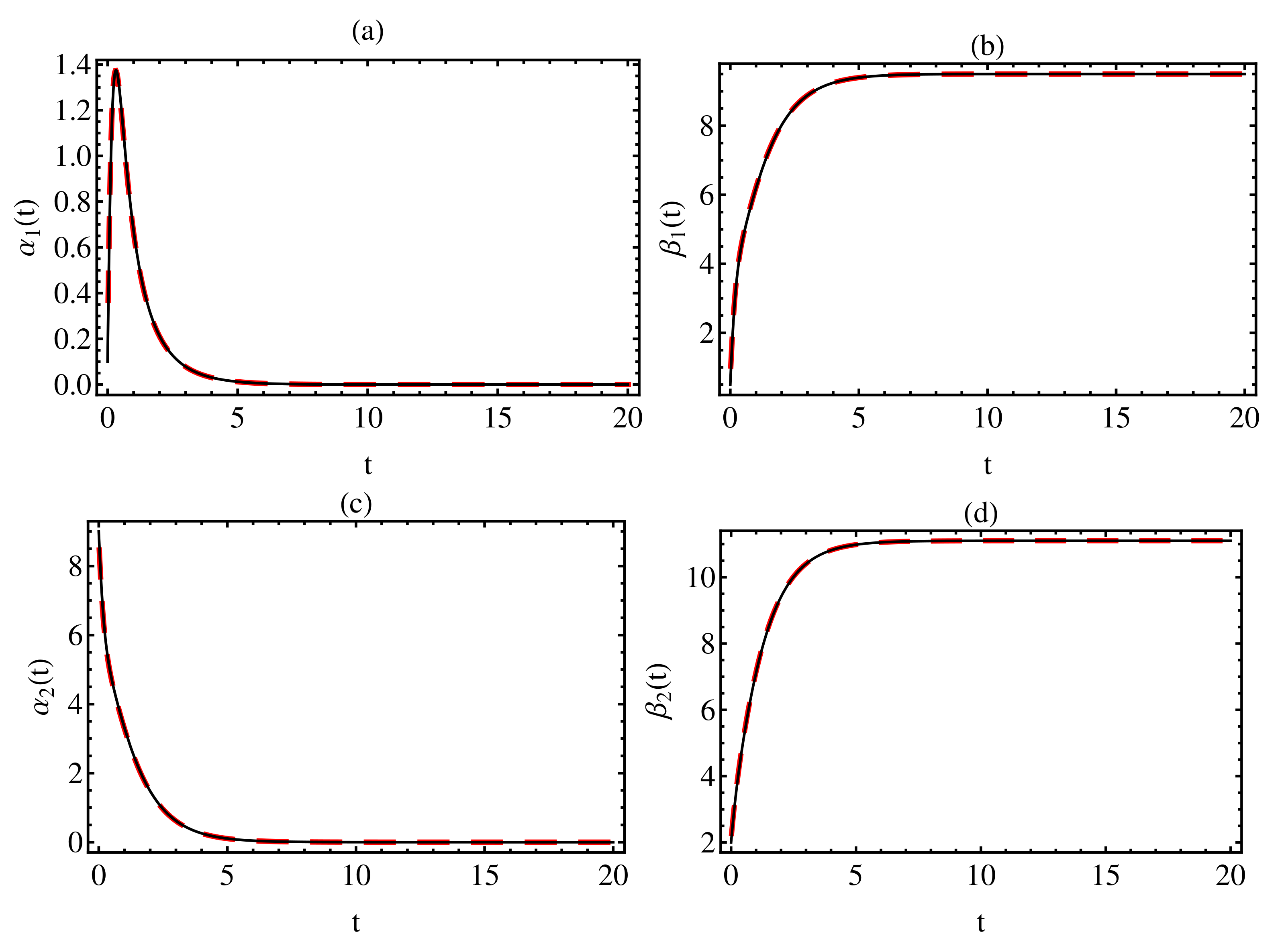
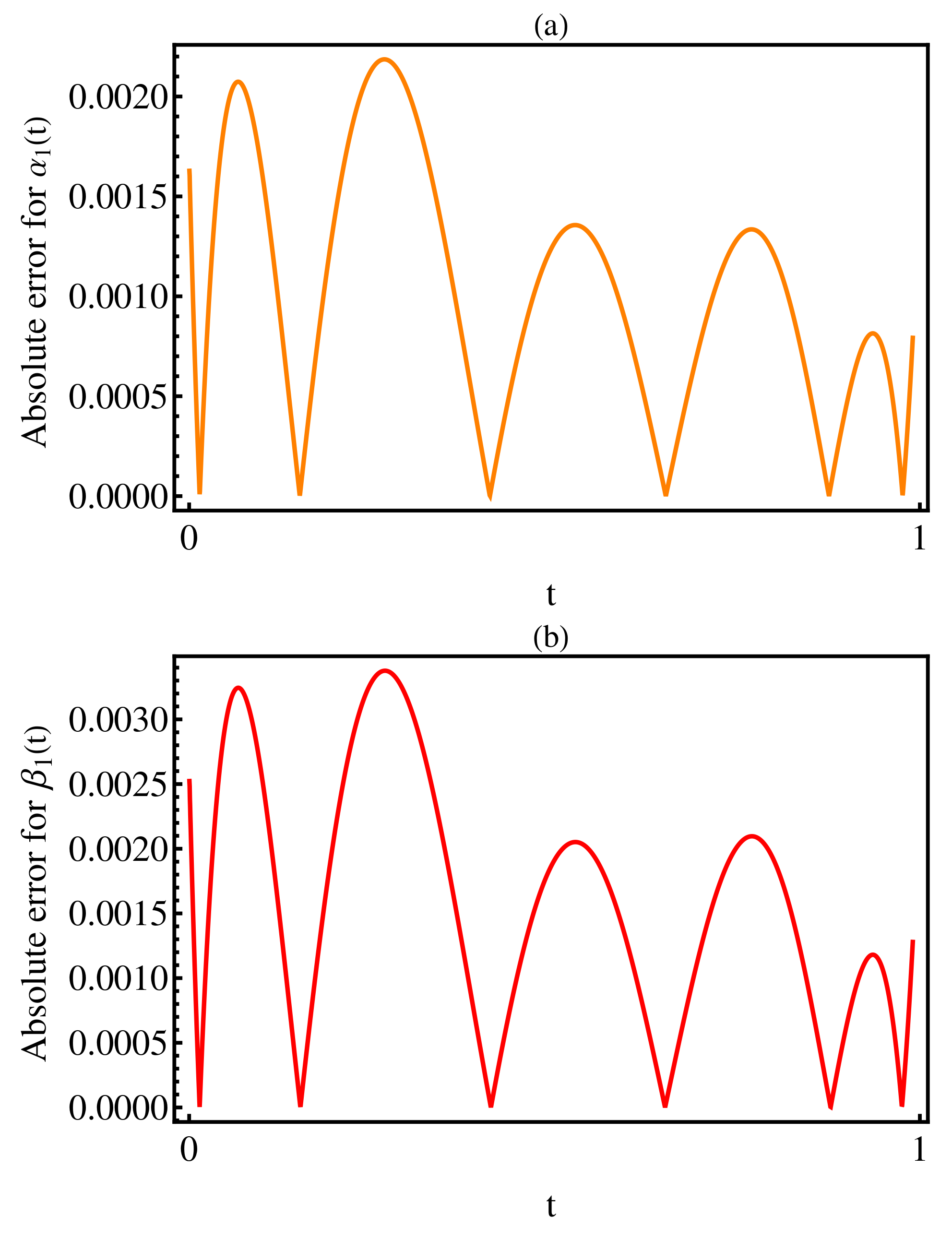
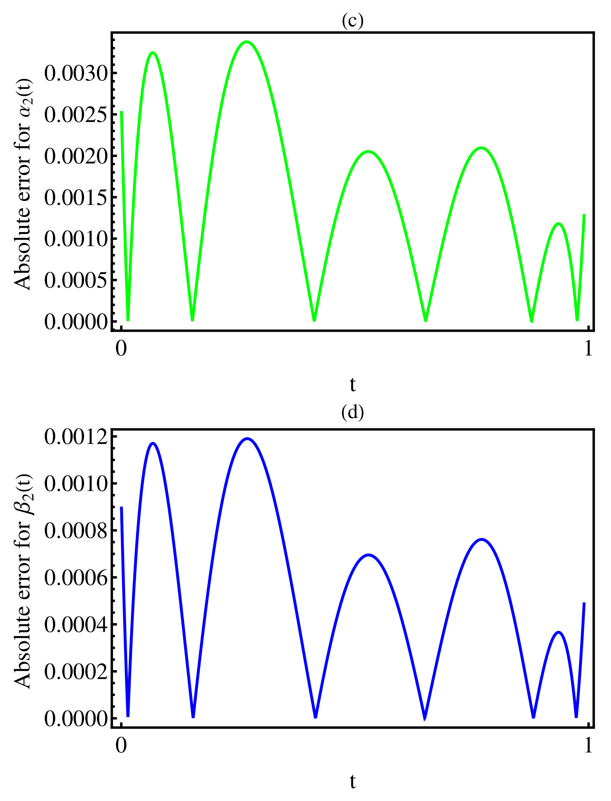
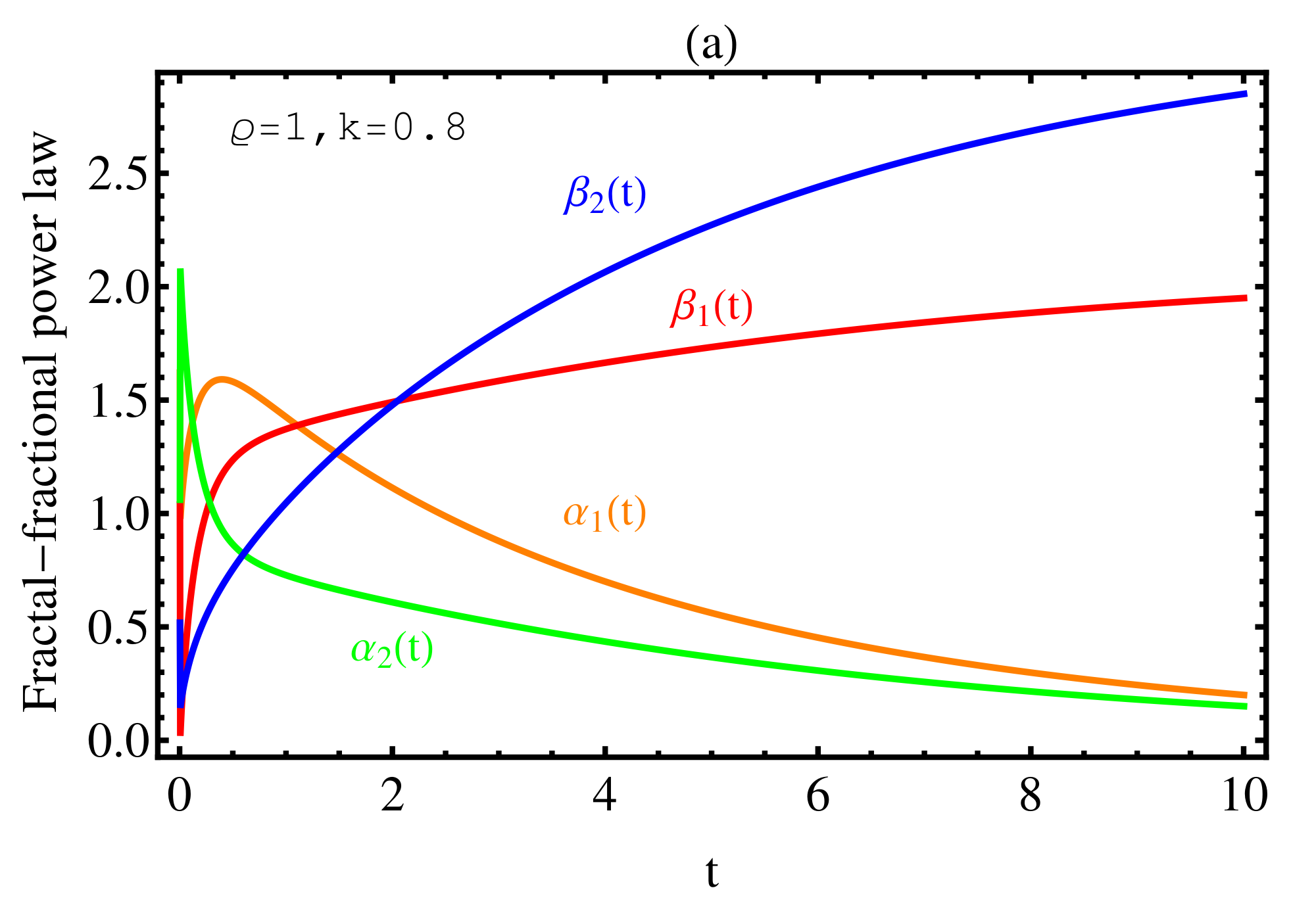
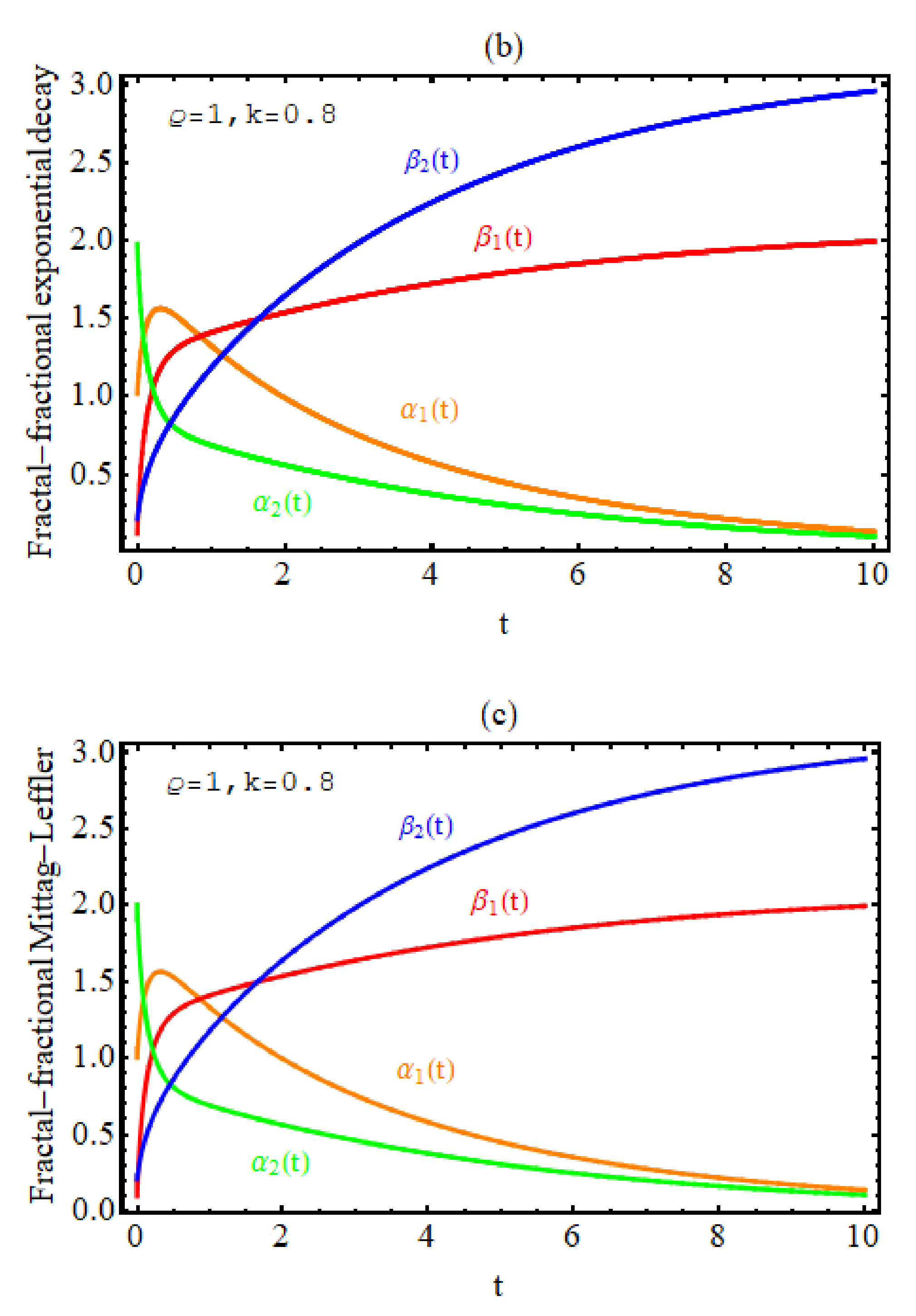
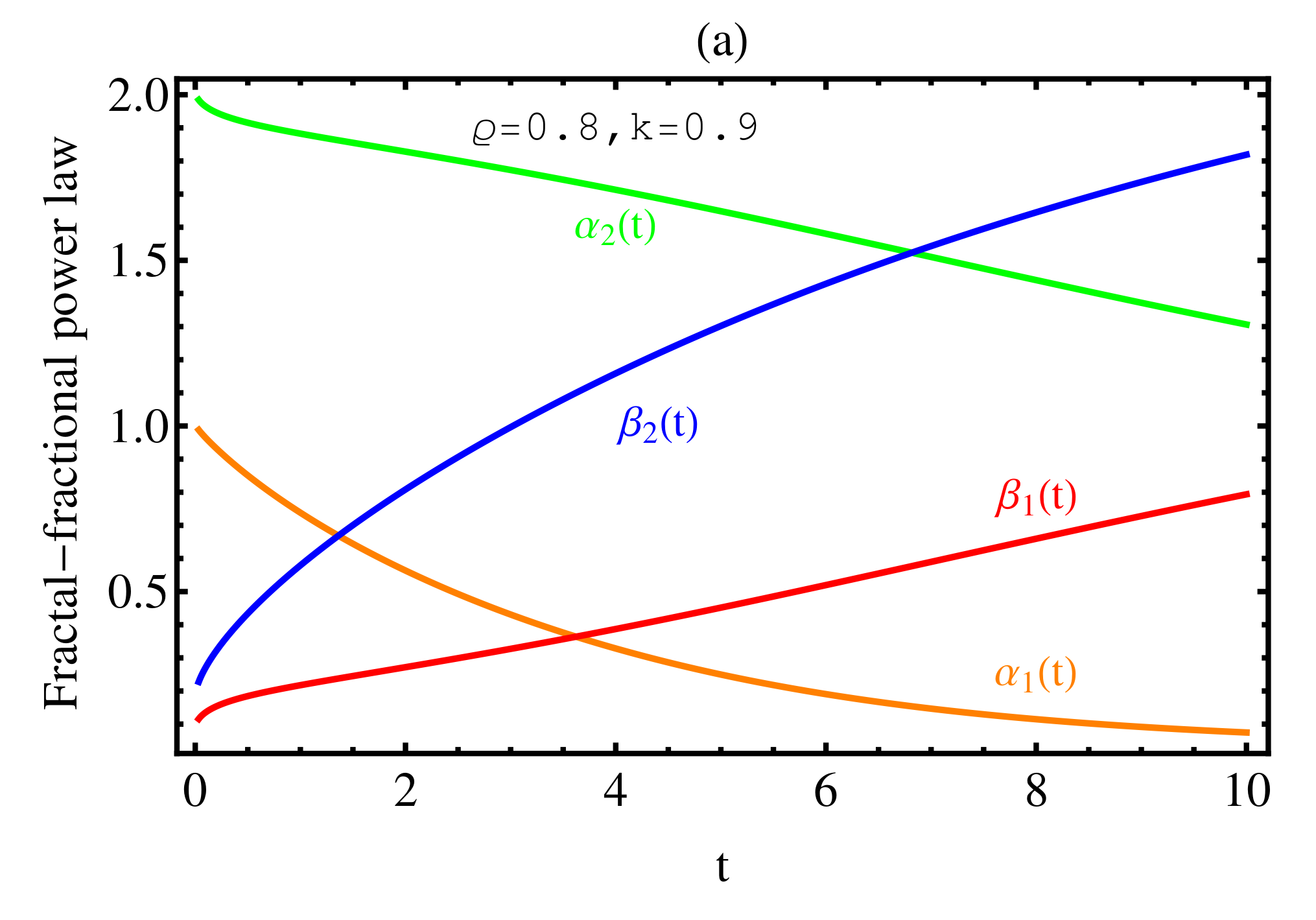
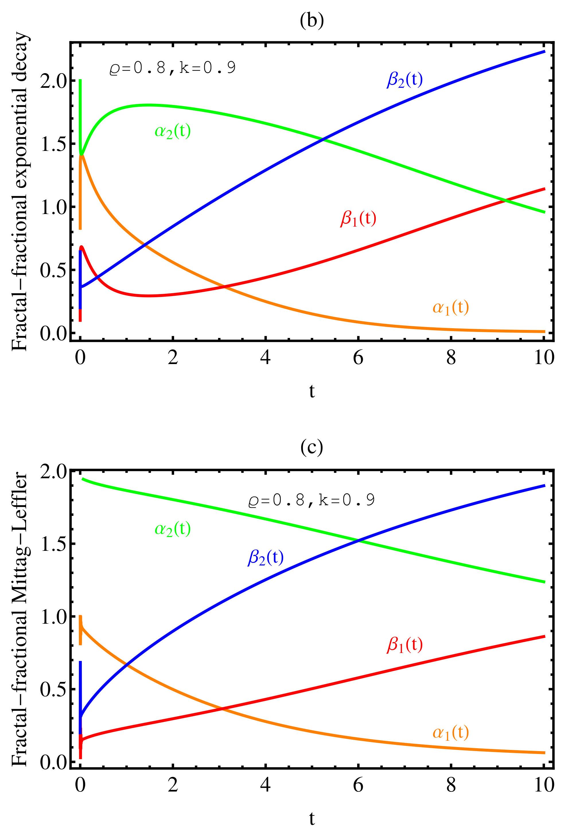
3. Numerical Results

In this section, we investigate the dynamics behavior and the numerical results of the concentration of a substrate, the concentration of an enzyme, the concentration of the resulting complex, and the concentration of the resulting product in the sense of fractal–fractional operators via power law, exponential decay, and Mittag-Leffler kernels or different fractal dimensions k and fractional order ϱ .
Figure 1 shows a comparison of the numerical solutions for Equations (36)–(39) of the concentration of the substrate, the concentration of an enzyme, the concentration of the resulting complex, and the concentration of the resulting product with the numerical solutions founded for those concentrations using the FDM.
In this figure, the initial conditions are α 1 ( 0 ) = 0.1 ,   β 1 ( 0 ) = 0.5 ,   α 2 ( 0 ) = 9 , and β 2 ( 0 ) = 2 , and the parameters values are δ = 1 ,   γ = 2 ,   σ = 1 , and h = 0.01 . Figure 2 shows the absolute error between the approximate solutions of Equations (82)–(85) and the approximation solutions in [24] according to the initial conditions α 1 ( 0 ) = 1 , β 1 ( 0 ) = 0.1 , α 2 ( 0 ) = 2 , and β 2 ( 0 ) = 0.2 . Here, the fractal dimension and fractional order are given by 0.8 and 0.9 , respectively, with δ = 1 , γ = 0.1 , σ = 0.2 , and h = 0.003 .
Figure 3 represents the behavior of the dynamics of the numerical solutions of Equations (36)–(39), (62)–(65), and (82)–(85) for the concentration of a substrate, the concentration of an enzyme, the concentration of the resulting complex, and the concentration of the resulting product via power law, exponential decay, and Mittag-Leffler kernels, in (a)–(c), respectively.
In this figure, we show the approximate solutions according to the initial conditions α 1 ( 0 ) = 1 , β 1 ( 0 ) = 0.1 , α 2 ( 0 ) = 2 , and β 2 ( 0 ) = 0.2 with ϱ = 1 , k = 0.8 , δ = 1 , γ = 2 , σ = 1 , and h = 0.003 .
In addition, Figure 4 shows the behavior of the dynamics of the numerical solutions of Equations (36)–(39), (62)–(65), and (82)–(85) with the same initial conditions and parameters as in Figure 3 but with ϱ = 0.8 , and k = 0.9 .

4. Discussion

In the last section, we illustrated the numerical results graphically through four figures via the the fractal–fractional Michaelis–Menten enzymatic reaction based on power law, exponential decay, and Mittag-Leffler kernels. Firstly, validity of the results is verified by comparing the numerical schemes of Equations (36)–(39) with the numerical results using the finite differences method when the fractal dimension and fractional order are integers. The comparison was made in the case of power-law kernel in Figure 1, when ϱ = 1 and k = 1 , due to the results, are very close to each other for all the schemes of Equations (36)–(39), (62)–(65), and (82)–(85). As for the verification in the case of the fractal dimension and fractional order, there are no previous studies that can be compared with it, except in the case of Mittag-Leffler kernel [24]. In Figure 2, the absolute error between our numerical results and the numerical results in [24] was illustrated. As seen from this figure, we can see the order of error is 10 3 . We can increase this order by increasing the iteration in our results and the terms in [24]. Despite this, the accuracy and effectiveness of the algorithm presented in this work, its accuracy and stability, in general, was verified in [23]. In Figure 3 and Figure 4, the effect of the fractal dimension and fractional order on the behavior of approximate solutions was studied. In Figure 3, we found that the strong coupling between α 1 and α 2 and β 1 and β 2 , besides all the approximate solutions, intersect with each other after a short time. In Figure 3, we noticed that there is no coupling between α 1 and α 2 and β 1 and β 2 , at least at the beginning of reactions. Additionally, we observed in Figure 3 that there is an oscillation at the beginning of the reaction, especially in the case of the existence of the exponential decay and Mittag-Leffler kernels.

5. Conclusions

We have proposed three new models of Michaelis–Menten enzymatic reaction by replacing the classical differential derivatives with fractal–fractional derivatives based on power law, exponential decay, and Mittag-Leffler kernels. The construction of the successive numerical iterations was obtained according to the theory of fractional calculus and with the help of Lagrangian interpolation for the three kernels. Validation of the numerical results based on power law in case of integer order compared with finite differences method was performed, and found excellent agreement in comparison with previous results in [24], in the case of fractal–fractional, and the error was of the order of 10 3 .
However, the comparison was only in the case of Mittag-Leffler kernel, due to the rarity or nonexistence of the studies carried out for the power-law and exponential decay kernels. Of course, what is meant by the previous studies is the sense of fractal–fractional differential. Hence, this is still a future goal for us and for many researchers, to develop many methods known in the sense of fractal-fraction differentials. Finally, the effects of the variety of values of the fractal dimension and fractional order on the dynamics of fractal–fractional enzymatic reaction were investigated with power law, exponential decay, and Mittag-Leffler kernels.
All calculations were performed using the Mathematica program.
In our future works, we propose to focus our attention on developing this study with the help of other special functions and spectral collocation methods. In addition, we can use Newton polynomial interpolation instead of Lagrange polynomial interpolation and obtain new results. Finally, due to the similarity of the rate equations we have used in this work to those associated with epidemiology and, in particular, the current COVID-19 pandemic, we will endeavor to extend our work to some models that are proposed in [32].

Author Contributions

M.A. performed the methodology, the software, and reviewed and edited the paper. K.M.S. suggested and initiated this work, performed the formal analysis of the investigation, the methodology, the software, and wrote the first draft of the paper. All authors have read and agreed to the published version of the manuscript.

Funding

The authors would like to express their gratitude to the Ministry of Education of Saudi Arabia and Najran University’s Deanship of Scientific Research for their financial and technical support under grant no. (NU/-/SERC/10/524).

Data Availability Statement

Not applicable.

Conflicts of Interest

The authors declare that there are no conflicts of interest regarding the publication of this paper.

References

  1. Shatey, S.; Motsa, S.S.; Khan, Y. A new piecewise spectral homotopy analysis of the Michaelis-Menten enzymatic reactions model. Numer. Algor. 2014, 66, 495–510. [Google Scholar] [CrossRef]
  2. Abu-Reesh, I.M. Optimal design of continuously stirred membrane reactors in series using Michaelis-Menten kinetics with competitive product inhibition: Theoretical analysis. Desalination 2005, 180, 119–132. [Google Scholar] [CrossRef]
  3. Golicnik, M. Explicit reformulations of time-dependent solution for a Michaelis-Menten enzyme reaction model. Anal. Biochem. 2010, 406, 94–96. [Google Scholar] [CrossRef] [PubMed]
  4. Golicnik, M. Evaluation of enzyme kinetic parameters using explicit analytic approximations to the Michaelis-Menten equation. Biochem. Eng. J. 2011, 53, 234–238. [Google Scholar] [CrossRef]
  5. Uma Maheswari, M.; Rajendran, L. Analytical solution of non-linear enzyme reaction equations arising in mathematical chemistry. J. Math. Chem. 2011, 49, 1713–1726. [Google Scholar] [CrossRef]
  6. Vogt, D. On approximate analytical solutions of differential equations in enzyme kinetics using homotopy perturbation method. J. Math. Chem. 2013, 51, 826–842. [Google Scholar] [CrossRef]
  7. Liang, S.; Jeffrey, D.J. Comparison of homotopy analysis method and homotopy perturbation method through an evolution equation. Commun. Nonlinear Sci. Numer. Simul. 2009, 14, 4057–4064. [Google Scholar] [CrossRef]
  8. Li, R.; Van Gorder, R.A.; Mallory, K.; Vajravelu, K. Solution method for the transformed time-dependent Michaelis–Menten enzymatic reaction model. J. Math. Chem. 2014, 52, 2494–2506. [Google Scholar] [CrossRef]
  9. Turkyilmazoglu, M. Some issues on HPM and HAM methods: A convergence scheme. Math. Comput. Model. 2011, 53, 1929–1936. [Google Scholar] [CrossRef]
  10. Alrabaiah, H.; Ali, A.; Haq, F.; Shah, K. Existence of fractional order semianalytical results for enzyme kinetics model. Adv. Differ. Equ. 2020, 2020, 443. [Google Scholar] [CrossRef]
  11. Liao, S.-J. On the homotopy analysis method for nonlinear problems. Appl. Math. Comput. 2004, 147, 499–513. [Google Scholar] [CrossRef]
  12. Saad, K.M.; AL-Shareef, E.H.F.; Alomari, A.K.; Baleanu, D.; Gómez-Aguilar, J.F. On exact solutions for timefractional Korteweg-de Vries and Korteweg-de Vries-Burgers equations using homotopy analysis transform method. Chin. J. Phys. 2020, 63, 149–162. [Google Scholar] [CrossRef]
  13. He, J.H. Variational iteration method-a kind of nonlinear analytical technique: Some examples. Int. J. Non-Linear Mech. 1999, 34, 699–708. [Google Scholar] [CrossRef]
  14. Shi, X.C.; Huang, L.L.; Zeng, Y. Fast Adomian decomposition method for the Cauchy problem of the time-fractional reaction diffusion equation. Adv. Mech. Eng. 2016, 8, 1–5. [Google Scholar] [CrossRef]
  15. Srivastava, H.M.; Saad, K.M. Some new and modified fractional analysis of the time-fractional Drinfeld–Sokolov–Wilson system. Chaos Interdiscip. J. Nonlinear Sci. 2020, 30, 113104. [Google Scholar] [CrossRef]
  16. Bueno-Orovio, A.; Kay, D.; Burrage, K. Fourier spectral methods for fractional-in-space reaction-diffusion equations. BIT Numer. Math. 2014, 54, 937–954. [Google Scholar] [CrossRef]
  17. Takeuchi, Y.; Yoshimoto, Y.; Suda, R. Second order accuracy fnite difference methods for space-fractional partial differential equations. J. Comput. Appl. Math. 2017, 320, 101–119. [Google Scholar] [CrossRef]
  18. Yildiray, Y.K.; Aydin, K. The solution of the Bagley Torvik equation with the generalized Taylor collocation method. J. Frankl. Inst. 2010, 347, 452–466. [Google Scholar]
  19. Saad, K.M.; Srivastava, H.M.; Gómez-Aguilar, J.F. A fractional quadratic autocatalysis associated with chemical clock reactions involving linear inhibition. Chaos Solitons Fractals 2020, 132, 109557. [Google Scholar] [CrossRef]
  20. Saad, K.M. Fractal-fractional Brusselator chemical reaction. Chaos Solitons Fractals 2021, 150, 111087. [Google Scholar] [CrossRef]
  21. Kilbas, A.A.; Srivastava, H.M.; Trujillo, J.J. Theory and Applications of Fractional Differential Equations; NorthHolland Mathematical Studies; Elsevier (North-Holland) Science Publishers: Amsterdam, The Netherlands; London, UK; New York, NY, USA, 2006; Volume 204. [Google Scholar]
  22. Podlubny, I. Fractional Differential Equations: An Introduction to Fractional Derivatives, Fractional Differential Equations, to Methods of Their Solution and Some of Their Applications; Mathematics in Science and Engineering; Academic Press: New York, NY, USA; London, UK; Sydney, Australia; Tokyo, Japan; Toronto, ON, Canada, 1999; Volume 198. [Google Scholar]
  23. Atangana, A. Fractal-fractional differentiation and integration: Connecting fractal calculus and fractional calculus to predict complex system. Chaos Solitons Fractals 2017, 102, 396–406. [Google Scholar] [CrossRef]
  24. Heydari, M.H.; Atangana, A.; Avazzadeh, Z.; Yang, Y. Numerical treatment of the strongly coupled nonlinear fractal-fractional Schr-dinger equations through the shifted Chebyshev cardinal functions. Alex. Eng. J. 2020, 59, 2037–2052. [Google Scholar] [CrossRef]
  25. Saad, K.M.; Alqhtania, M.; Gómez-Aguilarc, J.F. Fractal-fractional study of the hepatitis C virus infection model. Results Phys. 2020, 19, 103555. [Google Scholar] [CrossRef]
  26. Arfan, M.; Shah, K.; Ullah, A. Fractal-fractional mathematical model of four species comprising of prey-predation. Phys. Scr. 2021, 96, 124053. [Google Scholar] [CrossRef]
  27. LI, Z.; Liu, Z.; Khan, M.A. Fractional investigation of bank data with fractal-fractional Caputo derivative. Chaos Solitons Fractals 2020, 131, 109528. [Google Scholar] [CrossRef]
  28. Caputo, M. Linear models of dissipation whose Q is almost frequency independent: II. Geophys. J. Roy. Astron. Soc. 1967, 13, 529539. [Google Scholar] [CrossRef]
  29. Caputo, M.; Fabrizio, M. A new defnition of fractional derivative without singular kernel. Prog. Fract. Differ. Appl. 2015, 2, 73–85. [Google Scholar]
  30. Atangana, A.; Baleanu, D. New fractional derivative with nonlocal and non-singular kernel. Chaos Solitons Fractls Therm. Sci. 2016, 20, 757–763. [Google Scholar]
  31. Michaelis, L.; Menten, M.L. Die kinetik der invertinwirkung. Biochem. Z 1913, 49, 333–369. [Google Scholar]
  32. Agarwal, P.; Nieto, J.J.; Ruzhansky, M.; Torres, D.F.M. Analysis of Infectious Disease Problems (COVID-19) and Their Global Impact; Springer: Singapore, 2021. [Google Scholar]
Figure 1. Comparison between the numerical solutions of Equations (36)–(39) via power-law kernel and numerical solution based on finite differences method for ϱ = 1 ,   k = 1 ,   δ = 1 ,   γ = 2 ,   σ = 1 , and h = 0.01 . Black solid line: numerical solutions of Equations (36)–(39); red dashed line: numerical solutions of Equations (12)–(15) using finite differences method. (a) α 1 ( t ) , (b) β 1 ( t ) , (c) α 2 ( t ) , and (d) β 2 ( t ) .
Fractalfract 06 00013 g001
Figure 2. Absolute error between the numerical solutions of Equations (82)–(85) and [24] based on Mittag-Leffler kernel for ϱ = 0.9 ,   k = 0.8 ,   δ = 1 ,   γ = 2 ,   σ = 1 , and h = 0.0003 . (a) Absolute error for α 1 ( t ) , (b) Absolute error for β 1 ( t ) , (c) Absolute error for α 2 ( t ) , and (d) Absolute error for β 2 ( t ) .
Fractalfract 06 00013 g002aFractalfract 06 00013 g002b
Figure 3. The numerical solutions of the fractal–fractional Michaelis–Menten enzymatic reaction for ϱ = 1 ,   k = 0.8 ,   δ = 1 ,   γ = 2 ,   σ = 1 , and h = 0.003 . (a) The numerical solutions of Equations (36)–(39) based on power-law kernel; (b) The numerical solutions of Equations (62)–(65) based on exponential decay kernel; (c) The numerical solutions of Equations (82)–(85) based on Mittag-Leffler kernel (orange line: α 1 ( t ) ; red line: β 1 ( t ) ; green color: α 2 ( t ) ; blue line: β 2 ( t ) ) .
Fractalfract 06 00013 g003aFractalfract 06 00013 g003b
Figure 4. The numerical solutions of the fractal–fractional Michaelis-Menten enzymatic reaction for ϱ = 0.8 ,   k = 0.9 ,   δ = 1 ,   γ = 2 ,   σ = 1 , and h = 0.003 . (a) The numerical solutions of Equations (36)–(39) based on power-law kernel; (b) The numerical solutions of Equations (62)–(65) based on exponential decay kernel; (c) The numerical solutions of Equations (82)–(85) based on Mittag-Leffler kernel (orange line: α 1 ( t ) ; red line: β 1 ( t ) ; green line: α 2 ( t ) ; blue line: β 2 ( t ) ) .
Fractalfract 06 00013 g004aFractalfract 06 00013 g004b
Publisher’s Note: MDPI stays neutral with regard to jurisdictional claims in published maps and institutional affiliations.

