
Heat and Mass Transfer Impact on Differential Type Nanofluid with Carbon Nanotubes: A Study of Fractional Order System

 , , and
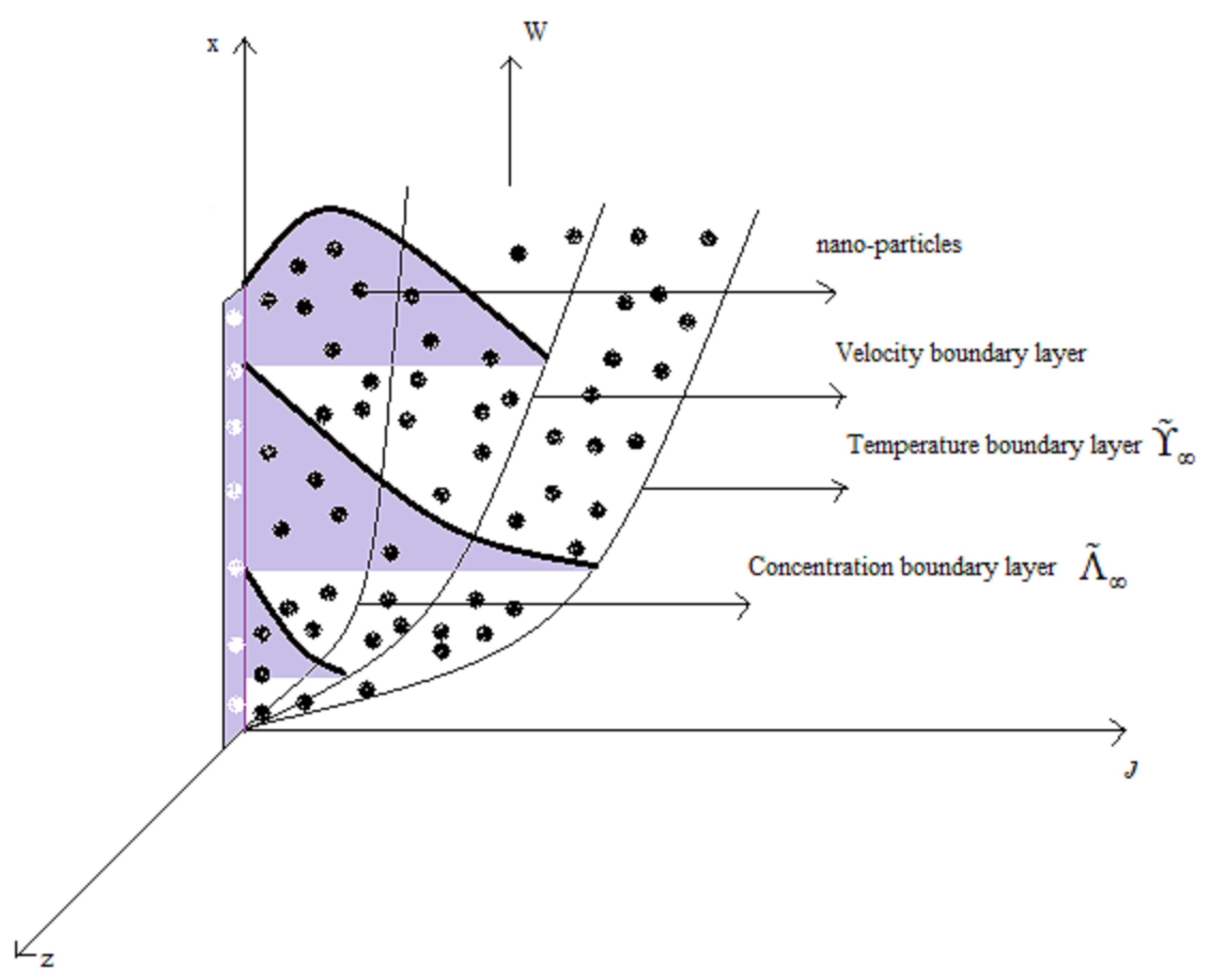
Abstract
:1. Introduction
2. Mathematical Model
Preliminaries
3. Solutions via Caputo
3.1. Temperature Profile
3.2. Concentration Profile
3.3. Velocity Profile
4. Solutions via Caputo–Fabrizio
4.1. Temperature Profile
4.2. Concentration Profile
4.3. Velocity Profile
5. Solutions via Atangana Baleanu
5.1. Temperature Profile
5.2. Concentration Profile
5.3. Velocity Profile
6. Results and Discussion
6.1. Effect of
6.2. Effect of
6.3. Effect of
6.4. Effect of P
6.5. Effect of
6.6. Effect of
6.7. Effect of
6.8. Effect of
6.9. Effect of
6.10. Effect of ℵ
6.11. Effect of
7. Conclusions
- Fluid flow descends for , P, , , ℵ and .
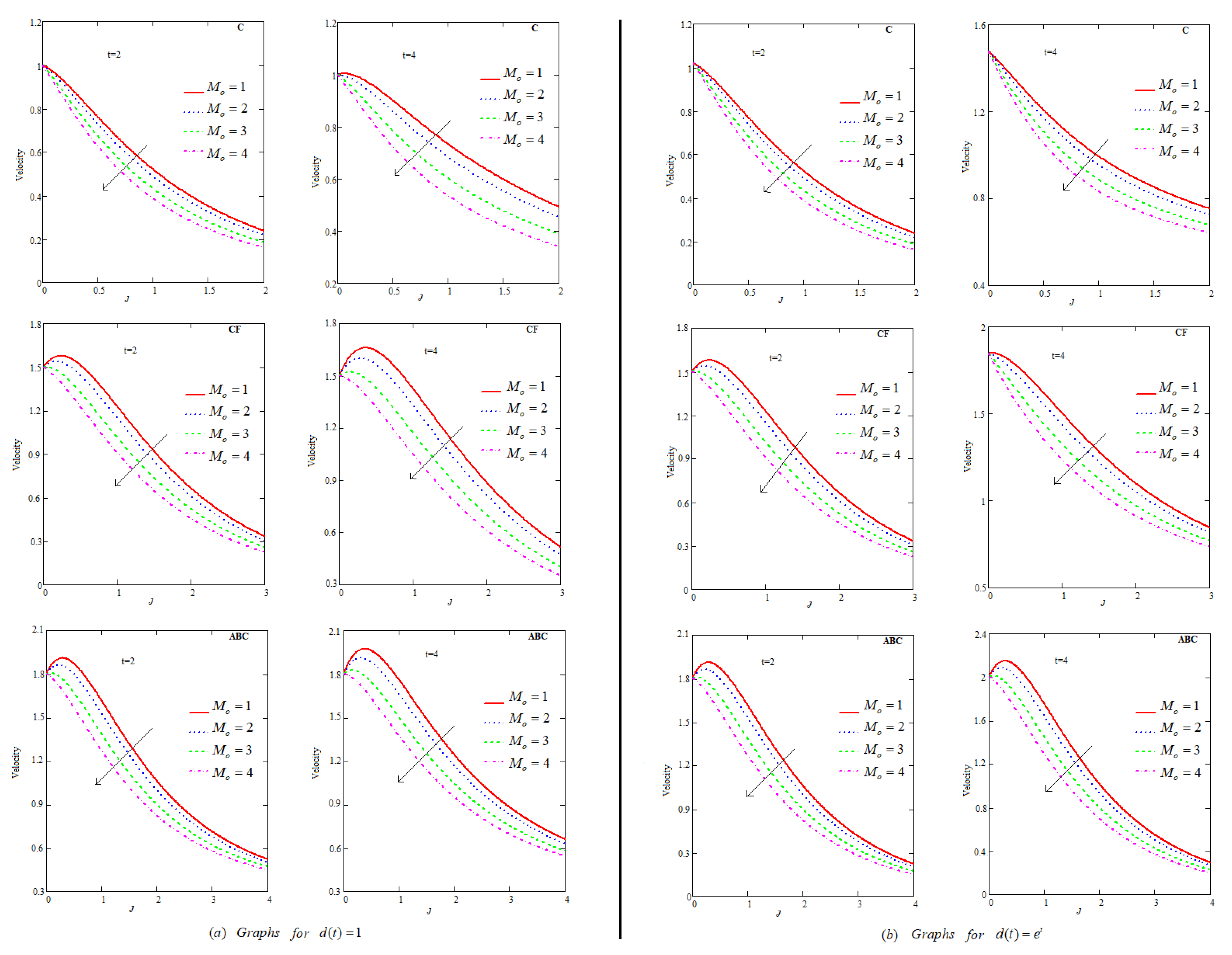
- Presence of resistive forces due to , fluid flow decelerates.
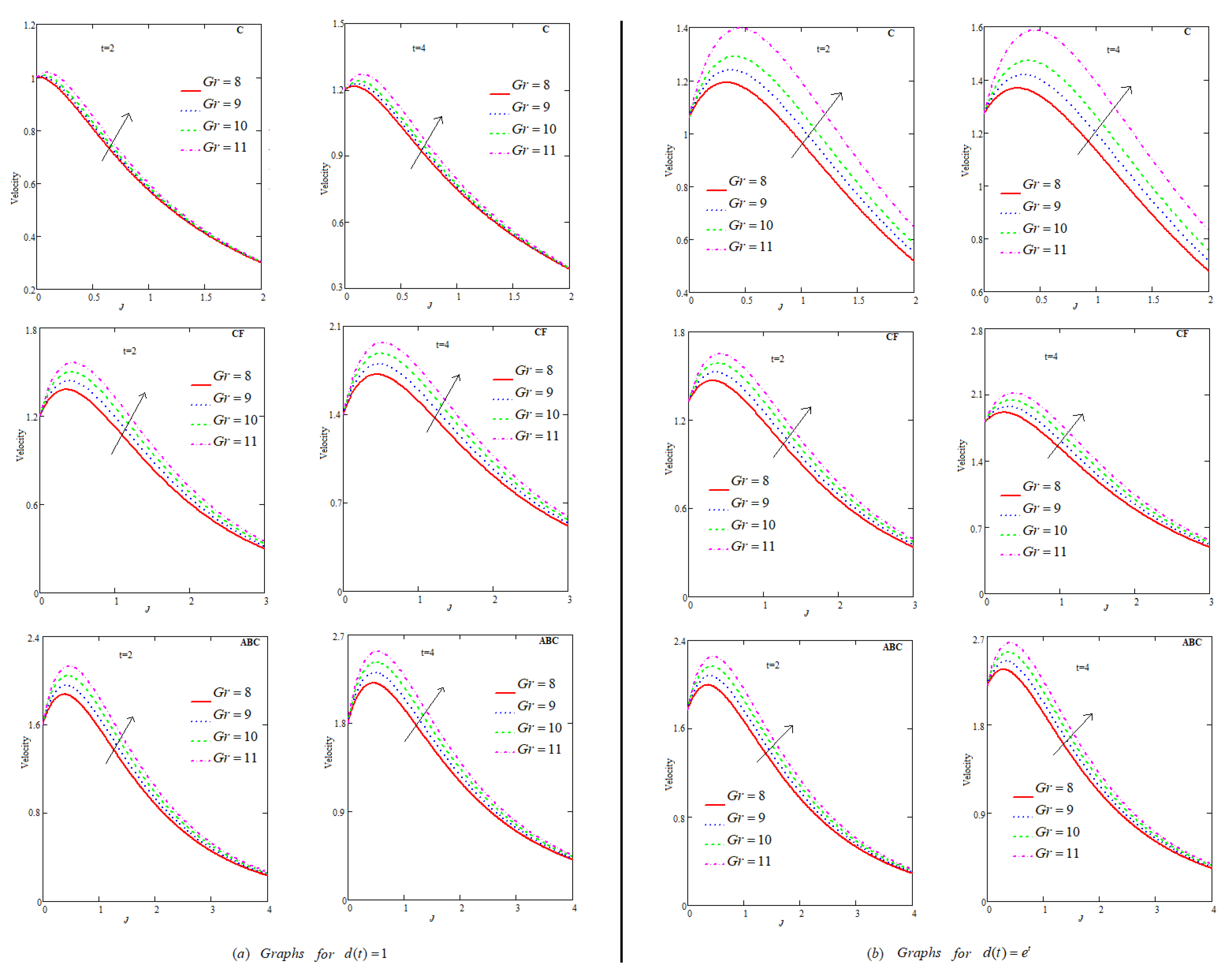
- Increment in flow field has been generated when , , and .
- For , velocity of nano-fluid escalates. Whereas for , flow’s velocity de-escalates.
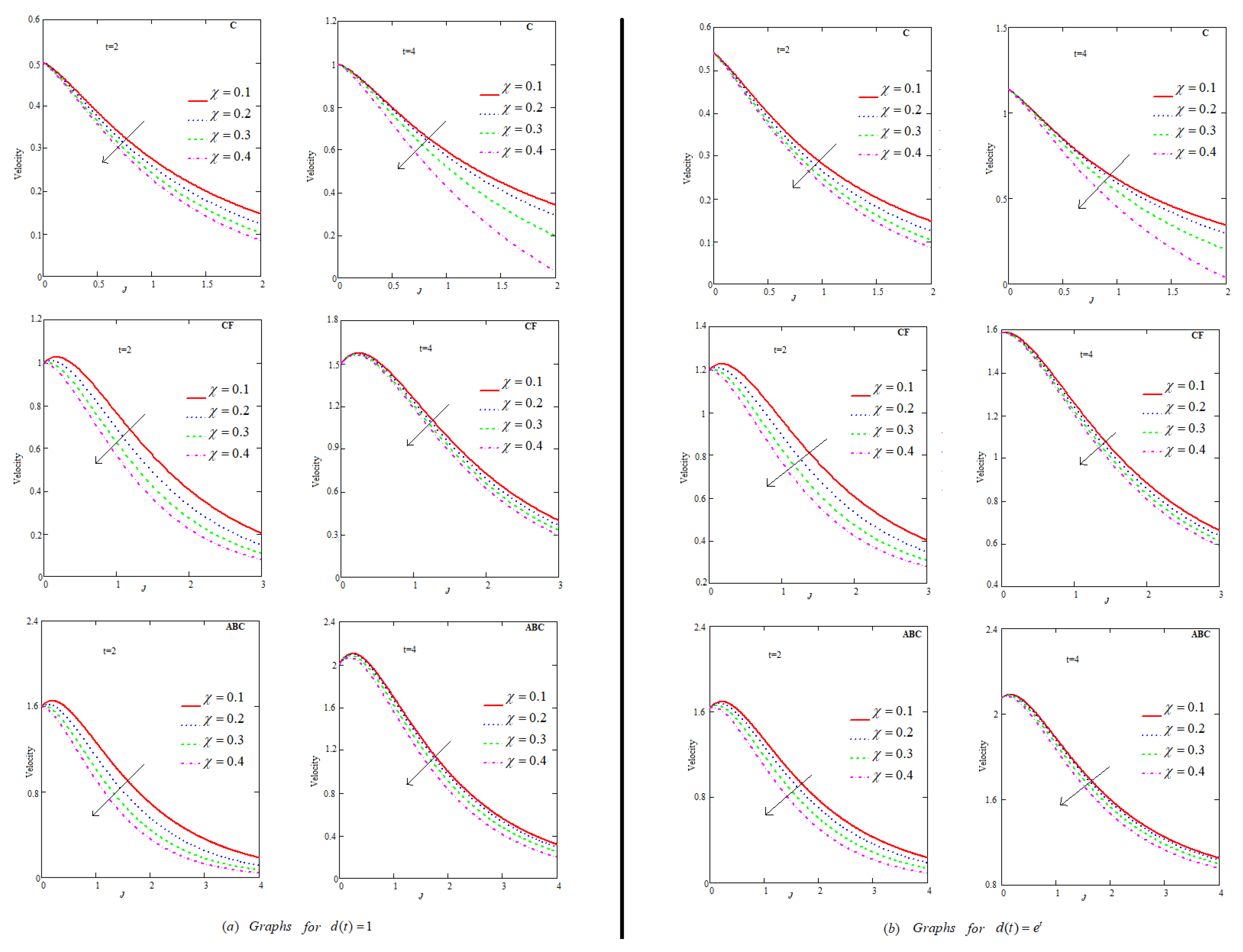
- Velocity of flow increases with increment in volumetric fraction for Caputo, Caputo–Fabrizio and Atangana–Baleanu models.
- Velocity profile is maximum when and minimum when .
- Among C, CF and ABC, flow profile is maximum for ABC.
Author Contributions
Funding
Institutional Review Board Statement
Informed Consent Statement
Data Availability Statement
Conflicts of Interest
Nomenclature
| Symbol | Quantity |
| Chemical reaction parameter | |
| h | Coefficient of heat transfer (WmK) |
| Concentration level on the plate (kgm) | |
| Concentration of the fluid far away from the plate (kgm) | |
| Constant suction velocity (s) | |
| Density of nano fluid (kgm) | |
| Dynamic viscosity of nano fluid (kgms) | |
| Fluid concentration (kgm) | |
| Fluid temperature (K) | |
| Fluid velocity (ms) | |
| Fractional parameter | |
| g | Gravitational acceleration (ms) |
| Heat generation | |
| Kinematic viscosity of nano fluid (ms) | |
| u | Laplace transforms parameter |
| Magnetic field | |
| Mass Grashof number | |
| Material constant or 2nd grade parameter | |
| Permitivity of medium | |
| ℘ | Porosity |
| Prandtl number | |
| Schmidt number | |
| Sherwood number | |
| Specific heat at constant temperature (jkgK) | |
| ℵ | Suction |
| Temperature of fluid at the plate (K) | |
| Temperature of fluid far away from the plate (K) | |
| k | Thermal conductivity of the fluid (WmK) |
| Thermal Grashof number | |
| Volumetric coefficient of expansion for mass concentration (mkg) | |
| Volumetric coefficient of thermal expansion (K) |
References
- Palani, G.; Abbas, I.A. Free convection MHD flow with thermal radiation from an impulsive started vertical plate. Non-Linear Anal. Model Control. 2009, 14, 73–84. [Google Scholar] [CrossRef] [Green Version]
- Kumar, B.R.; Sivaraj, R. Heat and mass transfer in MHD viscoelastic fluid flow over a vertical cone and flat plate with variable viscosity. Int. J. Heat Mass Trans. 2013, 56, 370–379. [Google Scholar] [CrossRef]
- Das, S.S.; Parija, S.; Padhy, R.K.; Sahu, M. Natural convection unsteady magneto-hydrodynamic mass transfer flow past an infinite vertical porous plate in presence of suction and heat sink. Int. J. Energy Environ. 2012, 3, 209–222. [Google Scholar]
- Atangana, A. On the new fractional derivative and application to nonlinear Fishers reaction-diffusion equation. Appl. Math. Comput. 2016, 273, 948–956. [Google Scholar]
- Tarasova, V.V.; Tarasov, V.E. Economic interpretation of fractional derivatives. Prog. Fract. Diff. Appl. 2017, 3, 1–7. [Google Scholar] [CrossRef]
- Yang, X.J.; Machado, J.A.T. A new fractional operator of variable order: Application in the description of anomalous diffusion. Phys. A 2017, 481, 276–283. [Google Scholar] [CrossRef] [Green Version]
- Zhuravkov, M.A.; Romanova, N.S. Review of methods and approaches for mechanical problem solutions based on fractional calculus. Math. Mech. Solids. 2016, 21, 595–620. [Google Scholar] [CrossRef]
- Cao, Z.; Zhao, J.; Wang, Z.; Liu, F.; Zheng, L. MHD flow and heat transfer of fractional Maxwell viscoelastic nanofluid over a moving plate. J. Mol. Liq. 2016, 222, 1121–1127. [Google Scholar] [CrossRef]
- Pandey, A.K.; Kumar, M. Effect of viscous dissipation and suction/injection on MHD nanofluid flow over a wedge with porous medium and slip. Alex. Eng. J. 2016, 55, 3115–3123. [Google Scholar] [CrossRef] [Green Version]
- Murshed, S.M.S.; Castro, C.A.N.D.; Lourenço, M.J.V.; Lopes, M.L.M.; Santos, F.J.V. A review of boiling and convective heat transfer with nanofluids. Renew. Sustain. Energy Rev. 2011, 15, 2342–2354. [Google Scholar] [CrossRef]
- Abro, K.A.; Khan, I.; Tassaddiq, A. Application of Atangana-Baleanu fractional derivative to convection flow of MHD Maxwell fluid in a porous medium over a vertical plate. Math. Model. Nat. Phen. 2018, 13, 1. [Google Scholar] [CrossRef] [Green Version]
- Saqib, M.; Kasim, A.R.M.; Mohammad, N.F.; Ching, D.L.C.; Shafie, S. Application of fractional derivative without singular and local kernel to enhanced heat transfer in CNTs nanofluid over an inclined plate. Symmetry 2020, 12, 768. [Google Scholar] [CrossRef]
- Wong, K.V.; Leon, O.D. Applications of nanofluids: Current and future. Nanotechnol. Energy 2017, 105–132. [Google Scholar]
- Lin, Y.H.; Kang, S.W.; Chen, H.L. Effect of silver nanofluid on pulsating heat pipe thermal performance. Appl. Therm. Eng. 2008, 28, 1312–1317. [Google Scholar] [CrossRef]
- Saqib, M.; Khan, I.; Shafie, S. Application of Atangana–Baleanu fractional derivative to MHD channel flow of CMC-based-CNT’s nanofluid through a porous medium. Chaos Solitons Fractals 2018, 116, 79–85. [Google Scholar] [CrossRef]
- Ikram, M.D.; Asjad, M.I.; Akgül, A.; Baleanu, D. Effects of hybrid nanofluid on novel fractional model of heat transfer flow between two parallel plates. Alex. Eng. J. 2021, 60, 3593–3604. [Google Scholar] [CrossRef]
- Maiti, S.; Shaw, S.; Shit, G.C. Fractional order model for thermochemical flow of blood with Dufour and Soret effects under magnetic and vibration environment. Colloids Surf. B Biointerfaces 2021, 197, 111395. [Google Scholar] [CrossRef]
- Sreedevi, P.; Reddy, P.S.; Rao, K.V.S.N.; Chamkhab, A.J. Heat and mass transfer flow over a vertical cone through nanofluid saturated porous medium under convective boundary condition suction/injection. J. Nanofluids 2017, 6, 478–486. [Google Scholar] [CrossRef]
- Du, M.; Wang, Z.; Hu, H. Measuring memory with the order of fractional derivative. Sci. Rep. 2013, 3, 3431. [Google Scholar] [CrossRef] [PubMed]
- Hayat, T.; Muhammad, T.; Shehzad, S.A.; Alsaedi, A. An analytical solution for magnetohydrodynamic Oldroyd-B nanofluid flow induced by a stretching sheet with heat generation/absorption. Int. J. Therm. Sci. 2017, 111, 274–288. [Google Scholar] [CrossRef]
- Ghalandari, M.; Maleki, A.; Haghighi, A.; Shadloo, M.S.; Nazari, M.A.; Tlili, I. Applications of nanofluids containing carbon nanotubes in solar energy systems: A review. J. Mol. Liq. 2020, 313, 113476. [Google Scholar] [CrossRef]
- Rao, Y. Nanofluids: Stability, phase diagram, rheology and applications. Particuology 2010, 8, 549–555. [Google Scholar] [CrossRef]
- Lim, A.E.; Lim, C.Y.; Lam, Y.C.; Taboryski, R. Electroosmotic flow in microchannel with black silicon nanostructures. Micromachines 2018, 9, 229. [Google Scholar] [CrossRef] [Green Version]
- Lim, A.E.; Lim, C.Y.; Lam, Y.C.; Taboryski, R.; Wang, S.R. Effect of nanostructures orientation on electroosmotic flow in a microfluidic channel. Nanotechnology 2017, 28, 255–303. [Google Scholar] [CrossRef] [Green Version]
- Alawi, O.A.; Mallah, A.R.; Kazi, S.N.; Sidik, N.A.; Najafi, G. Thermophysical properties and stability of carbon nanostructures and metallic oxides nanofluids. J. Therm. Anal. Calorim. 2019, 135, 1545–1562. [Google Scholar] [CrossRef]
- Pandikunta, S.; Tamalapakula, P.; Reddy, N.B. Inclined Lorentzian force effect on tangent hyperbolic radiative slip flow imbedded carbon nanotubes: Lie group analysis. J. Comput. Appl. Res. Mech. Eng. 2020, 10, 85–99. [Google Scholar]
- Aghamajidi, M.; Yazdi, M.; Dinarvand, S.; Pop, I. Tiwari-Das nanofluid model for magnetohydrodynamics (MHD) natural-convective flow of a nanofluid adjacent to a spinning down-pointing vertical cone. Propuls. Power Res. 2018, 7, 78–90. [Google Scholar] [CrossRef]
- Reddy, S.R.; Reddy, P.B.; Chamkha, A.J. Heat Transfer Analysis Of MHD CNTS Nanofluids Flow Over a Stretching Sheet. Spec. Top. Rev. Porous Media Int. J. 2020, 11, 133–147. [Google Scholar] [CrossRef]
- Upreti, H.; Rawat, S.K.; Kumar, M. Radiation and non-uniform heat sink/source effects on 2D MHD flow of CNTs-H2O nanofluid over a flat porous plate. Multidiscip. Model. Mater. Struct. 2019, 16, 791–809. [Google Scholar] [CrossRef]
- Upreti, H.; Pandey, A.K.; Kumar, M.; Makinde, O.D. Ohmic heating and non-uniform heat source/sink roles on 3D Darcy–Forchheimer flow of CNTs nanofluids over a stretching surface. Arab. J. Sci. Eng. 2020, 45, 7705–7717. [Google Scholar] [CrossRef]
- Hussain, Z.; Hayat, T.; Alsaedi, A.; Ahmad, B. Three-dimensional convective flow of CNTs nanofluids with heat generation/absorption effect: A numerical study. Comput. Methods App. Mech. Eng. 2018, 329, 40–54. [Google Scholar] [CrossRef]
- Alsagri, A.S.; Nasir, S.; Gul, T.; Islam, S.; Nisar, K.S.; Shah, Z.; Khan, I. MHD thin film flow and thermal analysis of blood with CNTs nanofluid. Coatings 2019, 9, 175. [Google Scholar] [CrossRef] [Green Version]
- Kumam, P.; Tassaddiq, A.; Watthayu, W.; Shah, Z.; Anwar, T. Modeling and simulation based investigation of unsteady MHD radiative flow of rate type fluid; a comparative fractional analysis. Math. Comput. Simul. 2021, in press. [Google Scholar]
- Saqib, M.; Khan, I.; Shafie, S.; Mohamad, A.Q. Shape effect on MHD flow of time fractional Ferro-Brinkman type nanofluid with ramped heating. Sci. Rep. 2021, 11, 3725. [Google Scholar] [CrossRef]
- Roohi, R.; Heydari, M.H.; Bavi, O.; Emdad, H. Chebyshev polynomials for generalized Couette flow of fractional Jeffrey nanofluid subjected to several thermochemical effects. Eng. Comput. 2021, 37, 579–595. [Google Scholar] [CrossRef]
- Maiti, S.; Shaw, S.; Shit, G.C. Fractional order model of thermo-solutal and magnetic nanoparticles transport for drug delivery applications. Colloids Surf. B Biointerfaces 2021, 203, 111754. [Google Scholar] [CrossRef]
- Abro, K.A. Role of fractal–fractional derivative on ferromagnetic fluid via fractal Laplace transform: A first problem via fractal–fractional differential operator. Eur. J. Mech-B/Fluids. 2021, 85, 76–81. [Google Scholar] [CrossRef]
- Ahmad, I.; Nazar, M.; Ahmad, M.; Nisa, Z.U.; Shah, N.A. MHD-free convection flow of CNTs differential type nanofluid over an infinite vertical plate with first-order chemical reaction, porous medium, and suction/injection. Math. Methods Appl. Sci. 2020. [Google Scholar] [CrossRef]
- Imran, M.A.; Khan, I.; Ahmad, M.; Shah, N.A.; Nazar, M. Heat and mass transport of differential type fluid with non-integer order time-fractional Caputo derivatives. J. Mol. Liq. 2017, 229, 67–75. [Google Scholar] [CrossRef]
- Al-Refai, M.; Abdeljawad, T. Analysis of the fractional diffusion equations with fractional derivative of non-singular kernel. Adv. Diff. Eq. 2017, 2017, 315. [Google Scholar] [CrossRef]
- Abdeljawad, T.; Baleanu, D. On fractional derivatives with generalized Mittag–Leffler kernels. Adv. Diff. Eq. 2018, 2018, 468. [Google Scholar] [CrossRef]
- Jarad, F.; Abdeljawad, T.; Hammouch, Z. On a class of ordinary differential equations in the frame of Atangana–Baleanu fractional derivative. Chaos Solitons Fractals 2018, 117, 16–20. [Google Scholar] [CrossRef]
- Stehfest, H.A. Numerical inversion of Laplace transforms. Commun. ACM 1970, 13, 9–47. [Google Scholar]


Publisher’s Note: MDPI stays neutral with regard to jurisdictional claims in published maps and institutional affiliations. |
© 2021 by the authors. Licensee MDPI, Basel, Switzerland. This article is an open access article distributed under the terms and conditions of the Creative Commons Attribution (CC BY) license (https://creativecommons.org/licenses/by/4.0/).
Share and Cite
Javed, F.; Riaz, M.B.; Iftikhar, N.; Awrejcewicz, J.; Akgül, A. Heat and Mass Transfer Impact on Differential Type Nanofluid with Carbon Nanotubes: A Study of Fractional Order System. Fractal Fract. 2021, 5, 231. https://doi.org/10.3390/fractalfract5040231
Javed F, Riaz MB, Iftikhar N, Awrejcewicz J, Akgül A. Heat and Mass Transfer Impact on Differential Type Nanofluid with Carbon Nanotubes: A Study of Fractional Order System. Fractal and Fractional. 2021; 5(4):231. https://doi.org/10.3390/fractalfract5040231
Chicago/Turabian StyleJaved, Fatima, Muhammad Bilal Riaz, Nazish Iftikhar, Jan Awrejcewicz, and Ali Akgül. 2021. "Heat and Mass Transfer Impact on Differential Type Nanofluid with Carbon Nanotubes: A Study of Fractional Order System" Fractal and Fractional 5, no. 4: 231. https://doi.org/10.3390/fractalfract5040231