
A Novel Analytical Approach for the Solution of Fractional-Order Diffusion-Wave Equations


Abstract
:1. Introduction
2. Preliminaries
3. ADM Implementation
4. New Idea Based on ADM
5. Numerical Results
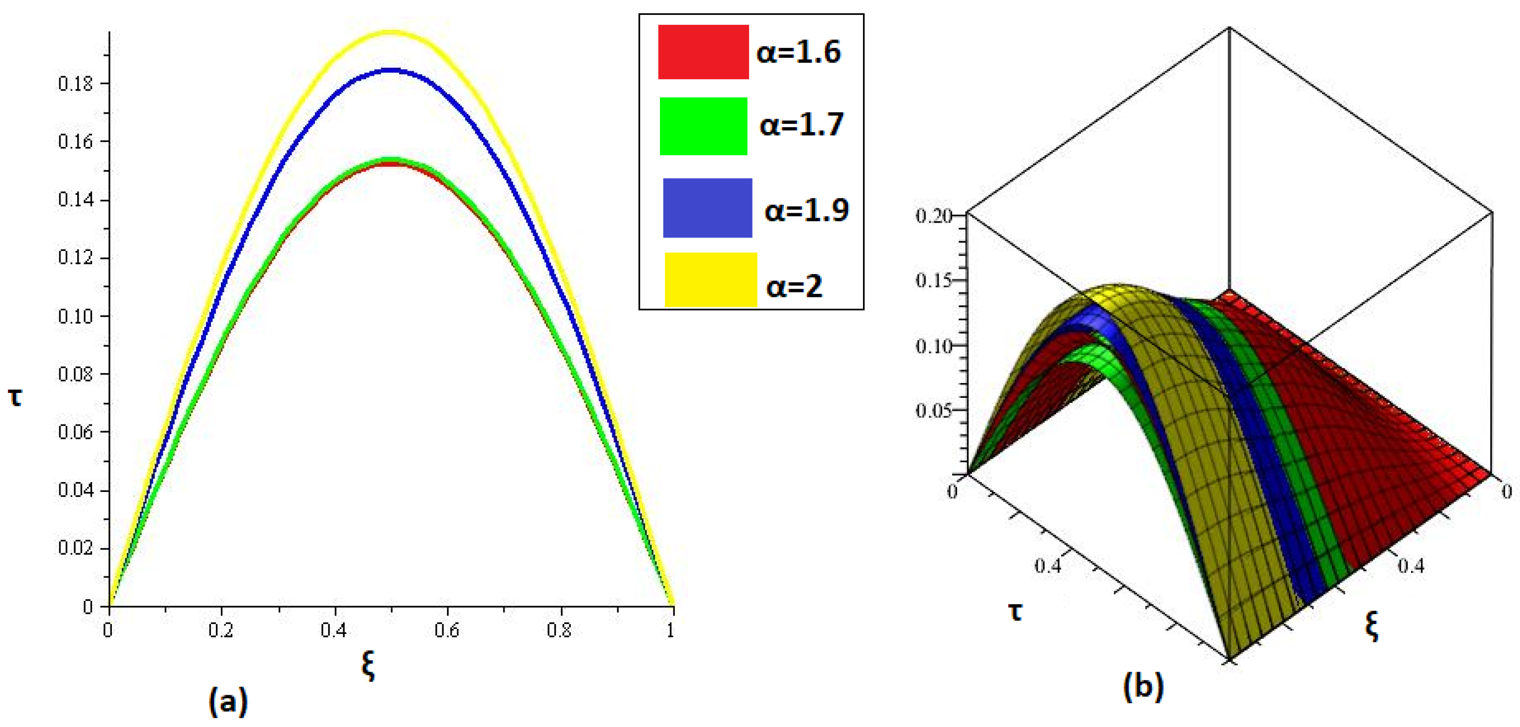
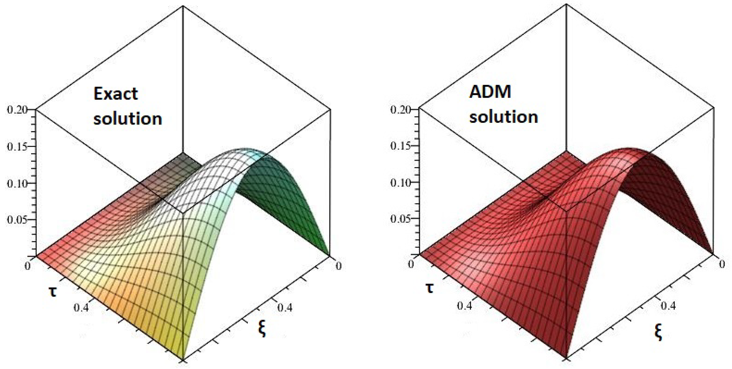
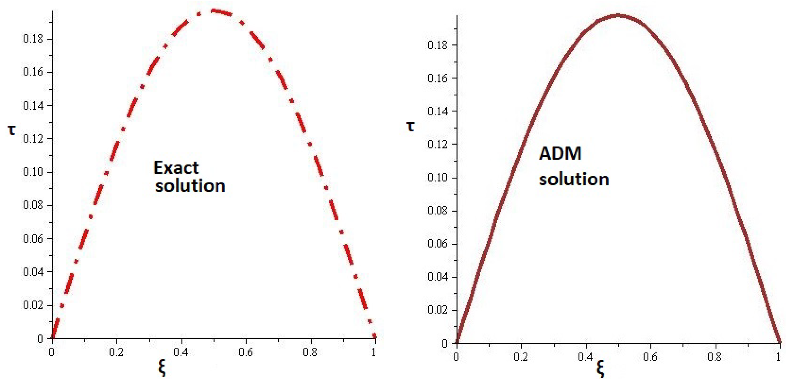
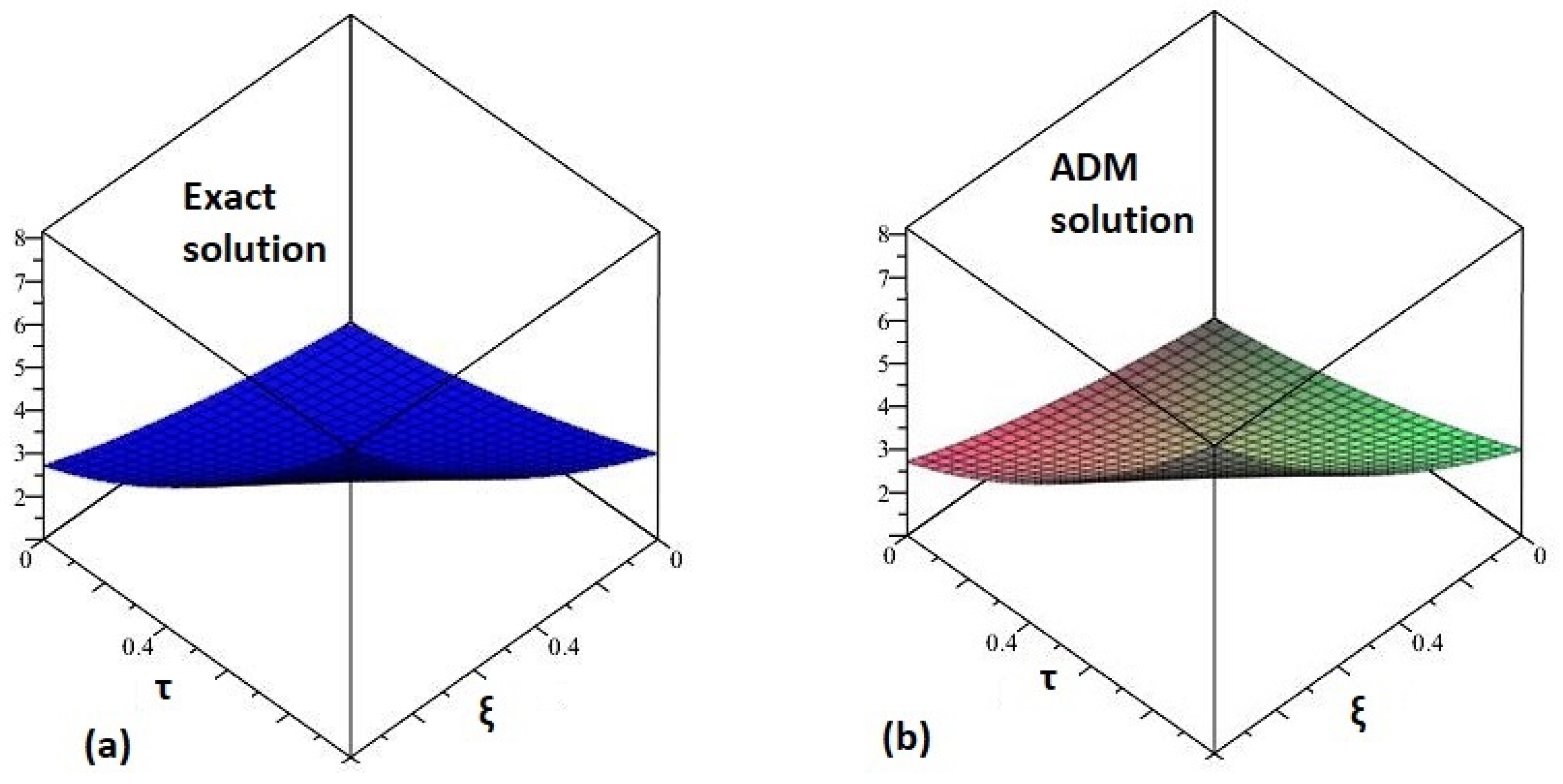
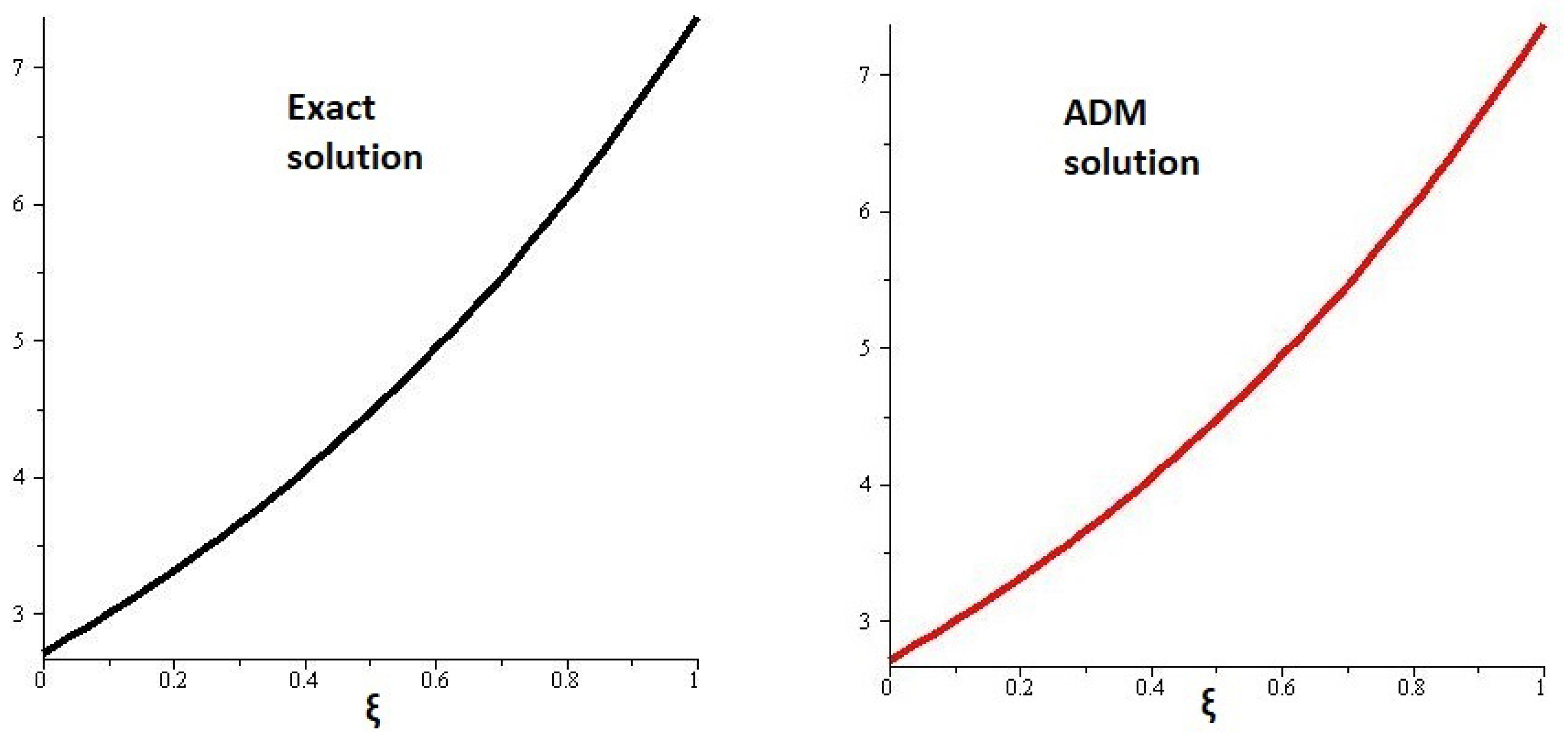
5.1. Example 1
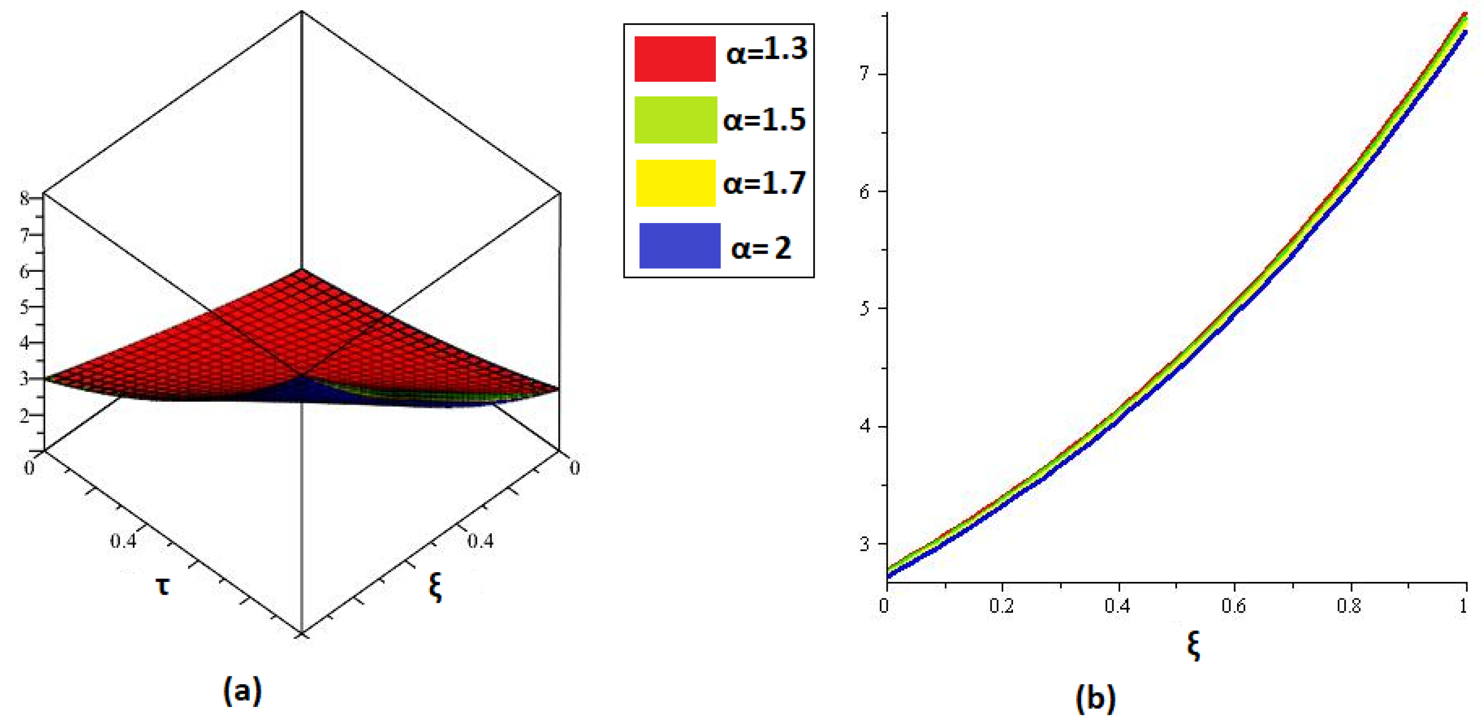
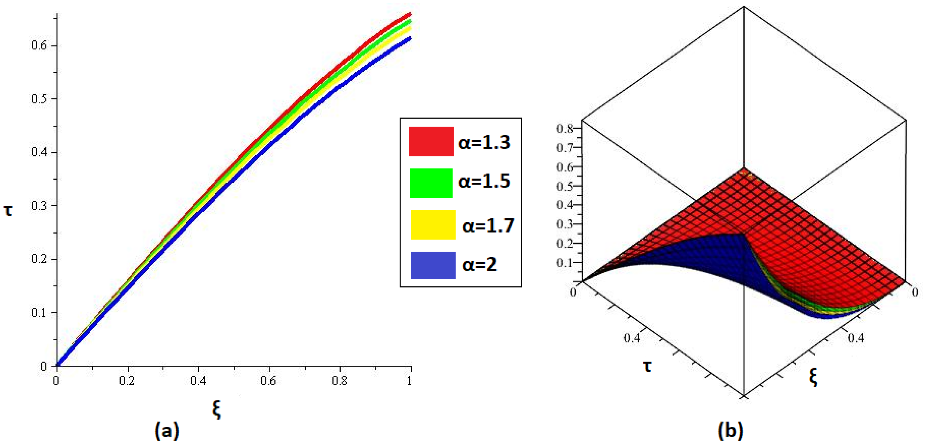
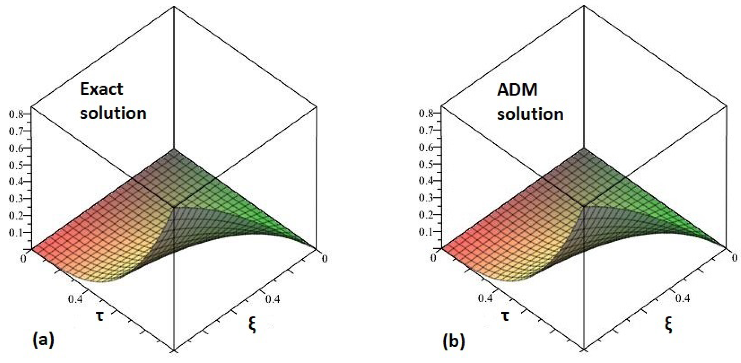
5.2. Example 2
5.3. Example 3
6. Conclusions
Author Contributions
Funding
Institutional Review Board Statement
Informed Consent Statement
Data Availability Statement
Conflicts of Interest
References
- Podlubny, I. Fractional Differential Equations: An Introduction to Fractional Derivatives, Fractional Differential Equations, to Methods of Their Solution and Some of Their Applications; Elsevier: Amsterdam, The Netherlands, 1998. [Google Scholar]
- Miller, K.S.; Ross, B. An Introduction to the Fractional Calculus and Fractional Differential Equations; Wiley: Hoboken, NJ, USA, 1993. [Google Scholar]
- Metzler, R.; Nonnenmacher, T.F. Space-and time-fractional diffusion and wave equations, fractional Fokker–Planck equations, and physical motivation. Chem. Phys. 2002, 284, 67–90. [Google Scholar] [CrossRef]
- Metzler, R.; Klafter, J. The random walk’s guide to anomalous diffusion: A fractional dynamics approach. Phys. Rep. 2000, 339, 1–77. [Google Scholar] [CrossRef]
- Debnath, L.; Bhatta, D.D. Solutions to few linear fractional inhomogeneous partial differential equations in fluid mechanics. Fract. Calc. Appl. Anal. 2004, 7, 21–36. [Google Scholar]
- He, J.H. Some applications of nonlinear fractional differential equations and their approximations. Bull. Sci. Technol. 1999, 15, 86–90. [Google Scholar]
- Turut, V.; Güzel, N. On solving partial differential equations of fractional order by using the variational iteration method and multivariate Padé approximations. Eur. J. Pure Appl. Math. 2013, 6, 147–171. [Google Scholar]
- Caputo, M. Linear models of dissipation whose Q is almost frequency independent—II. Geophys. J. Int. 1967, 13, 529–539. [Google Scholar] [CrossRef]
- Sharma, M. Fractional integration and fractional differentiation of the M-series. Fract. Calc. Appl. Anal. 2008, 11, 187–191. [Google Scholar]
- Rebenda, J.; Šmarda, Z. November. Numerical solution of fractional control problems via fractional differential transformation. In Proceedings of the 2017 European Conference on Electrical Engineering and Computer Science (EECS), Bern, Switzerland, 17–19 November 2017; pp. 107–111. [Google Scholar]
- Lei, Y.; Wang, H.; Chen, X.; Yang, X.; You, Z.; Dong, S.; Gao, J. Shear property, high-temperature rheological performance and low-temperature flexibility of asphalt mastics modified with bio-oil. Constr. Build. Mater. 2018, 174, 30–37. [Google Scholar] [CrossRef]
- Zhang, Z.Y. Symmetry determination and nonlinearization of a nonlinear time-fractional partial differential equation. Proc. R. Soc. 2020, 476, 20190564. [Google Scholar] [CrossRef] [Green Version]
- Gorenflo, R.; Mainardi, F.; Moretti, D.; Paradisi, P. Time fractional diffusion: A discrete random walk approach. Nonlinear Dyn. 2002, 29, 129–143. [Google Scholar] [CrossRef]
- Yang, Y.; Ma, Y.; Wang, L. Legendre polynomials operational matrix method for solving fractional partial differential equations with variable coefficients. Math. Probl. Eng. 2015, 2015, 915195. [Google Scholar] [CrossRef]
- Karimi, K.; Rostamy, D.; Mohamadi, E. Solving fractional partial differential equations by an efficient new basis. Int. J. Appl. Math. Comput. 2013, 5, 6–21. [Google Scholar]
- Magin, R.L. Fractional calculus in bioengineering, part 1. Crit. Rev. Biomed. Eng. 2004, 32. [Google Scholar] [CrossRef]
- Tarasov, V.E. Fractional integro-differential equations for electromagnetic waves in dielectric media. Theor. Math. Phys. 2009, 158, 355–359. [Google Scholar] [CrossRef] [Green Version]
- Magin, R.L. Fractional calculus in bioengineering, part 2. Crit. Rev. Biomed. Eng. 2004, 32. [Google Scholar] [CrossRef] [Green Version]
- Odibat, Z.; Momani, S. A generalized differential transform method for linear partial differential equations of fractional order. Appl. Math. Lett. 2008, 21, 194–199. [Google Scholar] [CrossRef] [Green Version]
- Yuanlu, L.I. Solving a nonlinear fractional differential equation using Chebyshev wavelets. Commun. Nonlinear Sci. Numer. Simul. 2010, 15, 2284–2292. [Google Scholar]
- Hosseini, V.R.; Shivanian, E.; Chen, W. Local radial point interpolation (MLRPI) method for solving time fractional diffusion-wave equation with damping. J. Comput. Phys. 2016, 312, 307–332. [Google Scholar] [CrossRef]
- Dehghan, M.; Abbaszadeh, M.; Mohebbi, A. Analysis of a meshless method for the time fractional diffusion-wave equation. Numer. Algorithms 2016, 73, 445–476. [Google Scholar] [CrossRef]
- Jia, J.; Wang, H. A preconditioned fast finite volume scheme for a fractional differential equation discretized on a locally refined composite mesh. J. Comput. Phys. 2015, 299, 842–862. [Google Scholar] [CrossRef] [Green Version]
- Hejazi, H.; Moroney, T.; Liu, F. Stability and convergence of a finite volume method for the space fractional advection–dispersion equation. J. Comput. Appl. Math. 2014, 255, 684–697. [Google Scholar] [CrossRef] [Green Version]
- Zhang, Y. A finite difference method for fractional partial differential equation. Appl. Math. Comput. 2009, 215, 524–529. [Google Scholar] [CrossRef]
- Chen, S.; Liu, F.; Zhuang, P.; Anh, V. Finite difference approximations for the fractional Fokker–Planck equation. Appl. Math. Model. 2009, 33, 256–273. [Google Scholar] [CrossRef] [Green Version]
- Jafari, H.; Seifi, S. Solving a system of nonlinear fractional partial differential equations using homotopy analysis method. Commun. Nonlinear Sci. Numer. Simul. 2009, 14, 1962–1969. [Google Scholar] [CrossRef]
- Saravanan, A.; Magesh, N. A comparison between the reduced differential transform method and the Adomian decomposition method for the Newell–Whitehead–Segel equation. J. Egypt. Math. Soc. 2013, 21, 259–265. [Google Scholar] [CrossRef] [Green Version]
- Lin, Y.; Xu, C. Finite difference/spectral approximations for the time-fractional diffusion equation. J. Comput. Phys. 2007, 225, 1533–1552. [Google Scholar] [CrossRef]
- Zhang, S.; Zhang, H.Q. Fractional sub-equation method and its applications to nonlinear fractional PDEs. Phys. Lett. A 2011, 375, 1069–1073. [Google Scholar] [CrossRef]
- Zheng, B. Exp-function method for solving fractional partial differential equations. Sci. World J. 2013, 2013, 465723. [Google Scholar] [CrossRef] [Green Version]
- Ghosh, U.; Sengupta, S.; Sarkar, S.; Das, S. Analytic solution of linear fractional differential equation with Jumarie derivative in term of Mittag-Leffler function. arXiv 2015, arXiv:1505.06514. [Google Scholar]
- Mainardi, F. Fractional Calculus And Waves in Linear Viscoelasticity: An Introduction To Mathematical Models; World Scientific: Singapore, 2010. [Google Scholar]
- Nigmatullin, R.R. The realization of the generalized transfer equation in a medium with fractal geometry. Phys. Status Solidi B 1986, 133, 425–430. [Google Scholar] [CrossRef]
- Meerschaert, M.M.; Benson, D.A.; Scheffler, H.P.; Baeumer, B. Stochastic solution of space-time fractional diffusion equations. Phys. Rev. E 2002, 65, 041103. [Google Scholar] [CrossRef] [Green Version]
- Agrawal, O.P. Response of a diffusion-wave system subjected to deterministic and stochastic fields. Z. Angew. Math. Mech. 2003, 83, 265–274. [Google Scholar] [CrossRef]
- Gorenflo, R.; Luchko, Y.; Mainardi, F. Wright functions as scale-invariant solutions of the diffusion-wave equation. J. Comput. Appl. Math. 2000, 118, 175–191. [Google Scholar] [CrossRef] [Green Version]
- Agrawal, O.P. A general solution for the fourth-order fractional diffusion-wave equation. Fract. Calc. Appl. Anal. 2000, 3, 1–12. [Google Scholar]
- Anh, V.V.; Leonenko, N.N. Harmonic analysis of random fractional diffusion–wave equations. Appl. Math. Comput. 2003, 141, 77–85. [Google Scholar] [CrossRef] [Green Version]
- Luchko, Y. Fractional wave equation and damped waves. J. Math. Phys. 2013, 54, 031505. [Google Scholar] [CrossRef] [Green Version]
- Luchko, Y. Wave-diffusion dualism of the neutral-fractional processes. J. Comput. Phys. 2015, 293, 40–52. [Google Scholar] [CrossRef]
- Luchko, Y. Initial-boundary-value problems for the one-dimensional time-fractional diffusion equation. Fract. Calc. Appl. Anal. 2012, 15, 141–160. [Google Scholar] [CrossRef] [Green Version]
- Sakamoto, K.; Yamamoto, M. Initial value/boundary value problems for fractional diffusion-wave equations and applications to some inverse problems. J. Math. Anal. Appl. 2011, 382, 426–447. [Google Scholar] [CrossRef] [Green Version]
- Kong, F.; Zhu, Q. New fixed-time synchronization control of discontinuous inertial neural networks via indefinite Lyapunov-Krasovskii functional method. Int. J. Robust Nonlinear Control 2021, 31, 471–495. [Google Scholar] [CrossRef]
- Jin, C.; Liu, M. A new modification of Adomian decomposition method for solving a kind of evolution equation. Appl. Math. Comput. 2005, 169, 953–962. [Google Scholar] [CrossRef]
- Pue-On, P.; Viriyapong, N. Modified Adomian decomposition method for solving particular third-order ordinary differential equations. Appl. Math. Sci. 2012, 6, 1463–1469. [Google Scholar]
- Hasan, Y.Q.; Zhu, L.M. Modified Adomian decomposition method for singular initial value problems in the second-order ordinary differential equations. Surv. Math. Appl. 2008, 3, 183–193. [Google Scholar]
- Jafari, H.; Daftardar-Gejji, V. Revised Adomian decomposition method for solving systems of ordinary and fractional differential equations. Appl. Math. Comput. 2006, 181, 598–608. [Google Scholar] [CrossRef]
- Khan, H.; Khan, A.; Kumam, P.; Baleanu, D.; Arif, M. An approximate analytical solution of the Navier–Stokes equations within Caputo operator and Elzaki transform decomposition method. Adv. Differ. Equ. 2020, 2020, 1–23. [Google Scholar]
- Shah, R.; Khan, H.; Arif, M.; Kumam, P. Application of Laplace–Adomian decomposition method for the analytical solution of third-order dispersive fractional partial differential equations. Entropy 2019, 21, 335. [Google Scholar] [CrossRef] [Green Version]
- Mahmood, S.; Shah, R.; Arif, M. Laplace Adomian decomposition method for multi dimensional time fractional model of Navier-Stokes equation. Symmetry 2019, 11, 149. [Google Scholar] [CrossRef] [Green Version]
- Shah, R.; Khan, H.; Mustafa, S.; Kumam, P.; Arif, M. Analytical Solutions of Fractional-Order Diffusion Equations by Natural Transform Decomposition Method. Entropy 2019, 21, 557. [Google Scholar] [CrossRef] [Green Version]
- Khan, H.; Shah, R.; Baleanu, D.; Kumam, P.; Arif, M. Analytical Solution of Fractional-Order Hyperbolic Telegraph Equation, Using Natural Transform Decomposition Method. Electronics 2019, 8, 1015. [Google Scholar] [CrossRef] [Green Version]
- Shah, R.; Farooq, U.; Khan, H.; Baleanu, D.; Kumam, P.; Arif, M. Fractional view analysis of third order Kortewege-De Vries equations, using a new analytical technique. Front. Phys. 2020, 7, 244. [Google Scholar] [CrossRef] [Green Version]
- Ali, I.; Khan, H.; Farooq, U.; Baleanu, D.; Kumam, P.; Arif, M. An Approximate-Analytical Solution to Analyze Fractional View of Telegraph Equations. IEEE Access 2020, 8, 25638–25649. [Google Scholar] [CrossRef]
- Momani, S.; Odibat, Z. Analytical solution of a time-fractional Navier–Stokes equation by Adomian decomposition method. Appl. Math. Comput. 2006, 177, 488–494. [Google Scholar] [CrossRef]
- Bildik, N.; Konuralp, A. Two-dimensional differential transform method, Adomian’s decomposition method, and variational iteration method for partial differential equations. Int. J. Comput. Math. 2006, 83, 973–987. [Google Scholar] [CrossRef]
- Oda, A.H.; Al, Q.; Lafta, H.F. Modified algorithm to compute Adomian’s polynomial for solving non-linear systems of partial differential equations. Int. Contemp. Math. Sci. 2010, 5, 2505–2521. [Google Scholar]
- Hashim, I. Adomian decomposition method for solving BVPs for fourth-order integro-differential equations. J. Comput. Appl. Math. 2006, 193, 658–664. [Google Scholar] [CrossRef] [Green Version]
- Wazwaz, A.M. The combined Laplace transform–Adomian decomposition method for handling nonlinear Volterra integro–differential equations. Appl. Math. Comput. 2010, 216, 1304–1309. [Google Scholar] [CrossRef]
- Abdou, M.A. Solitary Solutions of Nonlinear Differential-difference Equations via Adomain Decomposition Method. Int. J. Nonlinear Sci. 2011, 12, 29–35. [Google Scholar]
- Wang, Z.; Zou, L.; Zong, Z. Adomian decomposition and Padé approximate for solving differential-difference equation. Appl. Math. Comput. 2011, 218, 1371–1378. [Google Scholar] [CrossRef]
- Hosseini, M.M. Adomian decomposition method for solution of nonlinear differential algebraic equations. Appl. Math. Comput. 2006, 181, 1737–1744. [Google Scholar] [CrossRef]
- Hosseini, M.M. Adomian decomposition method for solution of differential-algebraic equations. J. Comput. Appl. Math. 2006, 197, 495–501. [Google Scholar] [CrossRef] [Green Version]
- Ali, E.J. A new technique of initial boundary value problems using Adomian decomposition method. Int. Math. Forum 2012, 7, 799–814. [Google Scholar]
- Ali, E.J. New Treatment of Initial Boundary Problems for Fourth-Order Parabolic Partial Differential Equations Using Variational Iteration Method. Int. J. Contemp. Math. Sci. 2011, 6, 2367–2376. [Google Scholar]
- Ali, E.J. New treatment of the solution of initial boundary value problems by using variational iteration method. Basrah J. Sci. 2012, 30, 57–74. [Google Scholar]
- Ahmed, A.A.I.; Ali, E.J.; Jassim, A.M. A new procedure of initial boundary value problems using homotopy perturbation method. J. Kufa Math. Comput. 2013, 1, 54–62. [Google Scholar]
- Alia, A.; Shaha, K.; Lib, Y.; Khana, R.A. Numerical treatment of coupled system of fractional order partial differential equations. J. Math. Comput. Sci. 2019, 19, 74–85. [Google Scholar] [CrossRef]
- Chen, A.; Li, C. Numerical solution of fractional diffusion-wave equation. Numer. Funct. Anal. Optim. 2016, 37, 19–39. [Google Scholar] [CrossRef]


| 0.1 | 2.469772 × 10 | 4.68002 × 10 | 3.2855 × 10 |
| 0.2 | 2.729520 × 10 | 5.17222 × 10 | 3.6311 × 10 |
| 0.3 | 3.016585 × 10 | 5.71619 × 10 | 4.0129 × 10 |
| 0.4 | 3.333843 × 10 | 6.31737 × 10 | 4.4351 × 10 |
| 0.5 | 3.684465 × 10 | 6.98177 × 10 | 4.9015 × 10 |
| 0.6 | 4.071964 × 10 | 7.71604 × 10 | 5.4170 × 10 |
| 0.7 | 4.500216 × 10 | 8.52755 × 10 | 5.9866 × 10 |
| 0.8 | 4.973509 × 10 | 9.42440 × 10 | 6.6163 × 10 |
| 0.9 | 5.496578 × 10 | 1.041558 × 10 | 7.3121 × 10 |
| 1 | 6.074659 × 10 | 1.151100 × 10 | 8.0812 × 10 |
Publisher’s Note: MDPI stays neutral with regard to jurisdictional claims in published maps and institutional affiliations. |
© 2021 by the authors. Licensee MDPI, Basel, Switzerland. This article is an open access article distributed under the terms and conditions of the Creative Commons Attribution (CC BY) license (https://creativecommons.org/licenses/by/4.0/).
Share and Cite
Mustafa, S.; Hajira; Khan, H.; Shah, R.; Masood, S. A Novel Analytical Approach for the Solution of Fractional-Order Diffusion-Wave Equations. Fractal Fract. 2021, 5, 206. https://doi.org/10.3390/fractalfract5040206
Mustafa S, Hajira, Khan H, Shah R, Masood S. A Novel Analytical Approach for the Solution of Fractional-Order Diffusion-Wave Equations. Fractal and Fractional. 2021; 5(4):206. https://doi.org/10.3390/fractalfract5040206
Chicago/Turabian StyleMustafa, Saima, Hajira, Hassan Khan, Rasool Shah, and Saadia Masood. 2021. "A Novel Analytical Approach for the Solution of Fractional-Order Diffusion-Wave Equations" Fractal and Fractional 5, no. 4: 206. https://doi.org/10.3390/fractalfract5040206