Unified Scale Theorem: A Mathematical Formulation of Scale in the Frame of Earth Observation Image Classification

Abstract

In this research, the geographic, observational, functional, and cartographic scale is unified into a single mathematical formulation for the purposes of earth observation image classification. Fractal analysis is used to define functional scales, which then are linked to the other concepts of scale using common equations and conditions. The proposed formulation is called Unified Scale Theorem (UST), and was assessed with Sentinel-2 image covering a variety of land uses from the broad area of Thessaloniki, Greece. Provided as an interactive excel spreadsheet, UST promotes objectivity, rapidity, and accuracy, thus facilitating optimal scale selection for image classification purposes.

1. Introduction

Scale is a term with multiple meanings in geospatial analysis [1]. Conceptually, scale represents the window of perception through which a landscape may be viewed or perceived [2]. In geosciences, scale concepts are considered as a critical factor when studying patterns in nature and the processes affecting them. In the context of remote sensing, objects and phenomena in the real world appear or are expressed in different ways depending on the scale of observation.

Overall, four concepts of “scale” have been recognized [3,4]:

• The geographic scale, defined by the extent of the study area;
• The observation (or measurement) scale (or resolution, or support), defined as the recording unit size (or pixel) of spectral reflectance in image data;
• The functional (or operational) scale, defined as the spatial or temporal window in which a feature is recognized or a process operates;
• The cartographic (or map) scale, defined as the ratio between a distance on a map and its corresponding distance in the real world—map scale is dictated by the capacity of the human eye for catching visual details on a map (according to the rule of thumb of half-a-millimeter distinction).

1.1. Image Classification and Scale

Optimal scale selection is crucial for image classification, and therefore, understanding how different concepts of scale relate to each other is fundamental. Image classification is the conversion of a continuous image (i.e., a spatially arranged spectral dataset) into a thematic layer. This is achieved by categorizing all pixels of the continuous image into a set of classes, or “themes”. The spectral pattern within the data for each pixel is used as the numerical basis for the categorization [5].

Image classification is a complex process, including the selection of a suitable classification system and nomenclature, the delineation of training and testing samples (or construction of rules), image preprocessing, the implementation of classification algorithms, possible post-classification processing, and accuracy assessment [6].

Among a variety of image classification methodologies, object-based classification is appropriate to describing the earth surface on different scales. The first step in object-based classification is object creation, resulting from image division into spatially continuous, disjointed and relatively homogeneous regions. There are several types of image segmentation algorithms [7,8].

Object-based classification facilitates the development of the hierarchical structure and the selection of appropriate nomenclature. Lu and Weng (2007) [6] have reported that object-based classification approaches demonstrate, in general, better performance than pixel-based approaches, especially when mapping individual landscape features. Karydas and Gitas (2011) [9] developed a rule-based classification algorithm for the object-based automated classification of rural landscapes using IKONOS imagery. Functioning on different scales, the algorithm organizes classes into three hierarchical levels. The overall accuracy was found to be 74%.

Dragut et al. (2014) [10] introduced an automated approach for the parameterization of the multi-scale image segmentation of multiple layers. The invented tool can run within eCognition^® software. The approach is based on the potential of local variance to detect scale transitions in geospatial data. The tool was tested with very high-resolution imagery, thus increasing objectivity and automation in object-based image analysis (OBIA). Similarly, Janowski et al. (2021) [11] developed a methodology for the extraction of secondary features from a digital elevation model, and employed feature selection using the Boruta algorithm, object-based image analysis, and random forest supervised classification for the mapping of glacial landforms.

Beyond OBIA, Parish and Duraisamy (2018) [12] provided a paradigm for multiscale modeling that combines the Mori–Zwanzig (MZ) formalism of statistical mechanics with the variational multiscale (VMS) method. This framework leads to a formally closed equation in which the effect of the unresolved scales on the resolved scales is non-local in time and appears as a convolution or memory integral.

1.2. Fractals and Scale Unification

Multiple scales in geosciences are strongly related to fractal geometry, as a fractal naturally involves many different scales, which, moreover, form a scaling hierarchy [13]. According to Lam et al. (2002) [14], fractal analysis is “an appropriate tool for detecting changes through scales in complex landscape process hierarchies”.

The fundamental characteristic of fractal features is that length, area, or volume are functions of the scale of measurement [15]. In the visual domain, fractals are recursive structures in which simple transformation rules generate hierarchies of infinite depth [16].

The potential usability of fractals in image analysis and classification has been addressed for some decades now. Hay et al. (2001) [17] showed that “image information is fractal in nature in terms of the same degree of non-regularity at all scales, or self-similarity across scales”. For a thorough investigation and review, see Lam et al. (2002) [18].

The use of fractal geometry by image analysis relies a lot on the estimation of fractal dimension (D), a key parameter introduced by Mandelbrot (1982) [19] in order to measure the irregularity of complex objects. Since then, several methods have been proposed to compute the fractal dimension of topographic surfaces or the image intensity surfaces [18,20,21,22,23].

Rather than using the fractal dimension in the strict sense [19], it is also possible to use it to summarize scale changes and thus relate or separate scales of variation that might be the result of particular natural processes [14]. In this direction, Berke (2010) [24] introduced the spectral fractal dimension (SFD) (a metric defined similarly to the original fractal dimension) to compare images for their spectral resolution and range, and thus assist in their classification. Jiang and Yin (2014) [13] introduced the ht-index as a metric of hierarchical structure complexity in geospatial datasets. The authors experimented with a grey-scale image, a digital elevation model, and road networks of different cities.

The possibility of linking multiple scales in remote sensing through fractals creates the basis for the unification of the different concepts of scale in geospatial analysis, and an image classification project offers the appropriate framework to conduct the unification.

1.3. Research Objectives

Unconvinced that nature would prescribe totally different modes of behavior for phenomena that were simply scaled differently, Albert Einstein sought a theory that would reconcile the two apparently irreconcilable theories: the general theory of relativity (on gravitation) and electromagnetism [25].

Although scale has been studied extensively in geosciences, unification of scale has not been attempted in the past. The objective of this research is to unify scale into a single mathematical formulation, through linking the different concepts of scale, namely geographic, observational, functional, and cartographic, within the frame of image classification.

The proposed unification is expected to facilitate the selection of optimal scale in image classification projects, which is usually based on intuition, experience, or trial-and-error approaches. The overall arrangement of scale unification conducted in the current work is called Unified Scale Theorem (UST).

2. Methodology

2.1. Background

The corner stone of Unified Scale Theorem (UST) is the detection of the functional scales of earth surface features in remote sensing images, and an appropriate methodology to achieve this goal is image segmentation. The objects created with segmentation correspond to real world features on different scales, and thus, the sizes of the objects derived from the optimal segmentation scales are considered (in a simplified manner) equivalent to their functional scales.

Karydas (2020) [26] has set up a method for detecting optimal scales when segmenting earth observation images using the fractal dimension as an optimality metric. Fractal Net Evolution Assessment (FNEA) is applied as a segmentation algorithm. The method has been proven mathematically, and was assessed with three different types of images (Sentinel-2, RapdiEye, and WorldView2). Karydas and Jiang (2020) [27] expanded the same methodology to raster topographic and hydrographic datasets.

To keep up with the work of Karydas (2020) [26], a part of the segmentation output is used in the current research for experimentation. The optimally defined objects are used as meaningful objects for training the classification algorithm and testing the classified images.

According to Karydas (2020) [26], the first step in defining the optimal segmentation scales—and thus the functional scales—is to partition the image via the rank-size rule (stemming from the Zipf’s law), thus dividing image data into a sequence of head and tail groups. Then, the detected optimal scales are transferred to the segmentation process by projecting the head groups of the partitions to the entire image; this has been described as a topological transformation. The criterion of scale optimality is that fractal dimension remains constant over rescaling.

The exact process of optimal segmentation scale detection follows the steps below (for details and further explanation, see Karydas 2020 [26] and Figure 1 in Karydas and Jiang 2020 [27]):

• Conversion of the original image into a principal component image and use of the PC1 layer;
• Multi-resolution segmentation of the PC1 layer, using the Fractal Net Evolution Assessment (FNEA) algorithm (embedded in eCognition software) for a series of scale factors (f). The scale factor corresponds to the standard deviation of spectral information inside a candidate object, and is the most influencing input parameter in segmentation;
• Plotting of the scale factor values (f) vs. the resulting mean object size values (s_f) and extraction of a power-law equation from the plotted data;
• Application of the rank-size rule with the PC1 layer. Then, extraction of the head–tail portions per partition according to the paradigm of the “ht-index” (Jiang and Yin, 2014);
• In the partition table, computation of the “simulated mean object size” (s_n) at every partition level. s_n is the ratio of the total image extent to the extent of the head group at that partition level;
• Computation of the optimal segmentation scale (f_n) for each partition level by resolving the extracted power-law equation.

Apart from being used as an optimality metric in the mathematical proof of Karydas (2020) [26], fractals are directly involved in the implemented segmentation process. Bobick and Bolles (1992) [28] argue that the information stored in an image with FNEA is considered as fractal in terms of holding the same degree of non-regularity at all scales, or (inversely) self-similarity across every scale.

2.2. Mathematical Formulation

For a set of optimal scales as indicated by Karydas (2020) [26], the mean feature size per scale—and thus, the functional scales—can be computed according to the defined power-law equation, as follows:

$$s_n =\mathrm{a} {f_n}^{\mathrm{b}}$$

(1)

where s_n is the mean feature size (in m²) at scale n; f_n is the scale factor value; a and b are constants. Then, the radius of the mean feature (${s_n}^{\prime }$) is defined as:

$${s_n}^{\prime } =\sqrt{\raisebox{1ex}{$s_n$}\!\left/ \!\raisebox{-1ex}{$\pi $}\right.}$$

(2)

From the functional scales, the cartographic scales can also be determined using the rule of thumb according to which the human eye cannot recognize objects smaller than 0.5 mm on a map:

$$C_n=\raisebox{1ex}{${s_n}^{\prime }$}\!\left/ \!\raisebox{-1ex}{$0.0005$}\right.$$

(3)

where $C_n$ is the denominator of the cartographic scale for scale n; ${s_n}^{\prime }$ is the mean feature radius (in m) for scale n.

From the range of resulting cartographic values corresponding to different targeted spatial features, the most appropriate cartographic scale will be determined by the specific requirements and limitations of the classification project. Finally, from the exact cartographic scale value, a nominal cartographic scale can be assigned by replacing the denominator with a close rounded number (e.g., 1/17,452 → 1/15,000).

Together with Equations (1)–(3), a set of three conditions is also defined, describing some more or less obvious limitations:

• Condition-1—The pixel size of the image in hand must be smaller than the mean feature size of the smallest functional scale. Otherwise, the smallest functional scale must be rejected;
• Condition-2—The number of objects on the largest functional scale must be greater than one. The number of objects for every scale is defined by dividing the size of the image in hand with the mean feature size on that scale;
• Condition-3—The final cartographic scale must be greater than 1.

With an image in hand, the resolution and the study area are predefined. Then, the size of the study area indicates the geographic scale of the project, while image segmentation will allow the definition of the functional scales (f_n) (using Equations (1) and (2)), from which the cartographic scale will in turn be determined (using Equation (3)). This approach is supportive of “feature-based” classification, whereby the properties of the spatial features may define the classification nomenclature.

Inversely, if the cartographic scale is predefined, the feature mean size—and thus, the functional scale and the optimal resolution—can be estimated using the following equation (derived after replacing ${s_n}^{\prime }$ in Equation (3) with that from Equation (2)):

$$s_n=0.785 {(C/1000)}^2$$

(4)

The latter approach is supportive of a “nomenclature-based” classification, where spatial features are forced to comply with predefined classes by the classification nomenclature. Again, the geographic scale of the project is indicated by the study area.

2.3. Scale Calculator

The entire set of Equations (1)–(3), together with Conditions-1, -2, and -3 and the segmentation process outputs, are prescribed in a dynamic excel spreadsheet, which can be used as scale calculator.

The cells are grouped vertically into four areas, one per scale concept (Geographic, Observation, Functional, and Cartographic), while the equations and conditions are indicated accordingly.

Conversions and computations are conducted automatically after the basic input parameters (image size and resolution) are declared, while the outputs of the segmentation process (constants of the power-law equation and indicated optimal scale factors) are entered.

The calculator can serve both classification approaches, i.e., the “feature-based” and the “nomenclature-based” classification. The UST scale calculator is available (as an excel file) to any potential user (

Table 1. The Excel spreadsheet of the scale calculator in function view.

	A	B	C	D	E	F	G	H	I	J
1	Geographic Scale	Observation Scale	Functional Scale					Cartographic Scale
2	Image size (m2)	Pixel (m)	Equation (2)
3	INPUT VALUE	INPUT VALUE	Min mean feature size					Equation (3)		Rule of thumb
4	Image side (m)	Surface (m2)	=SQRT(C5/3.14)	Radius (m)				1/	=C15/J15	0.0005
5	=SQRT(A3)	=B3 × B3	=C10	Surface (m2)				Nominal scale	=((INT(I4/10,000) + 1) × 10,000) − 5000	Condition-3
6			Max number of objects							Nominal scale > 1
7	Condition-2	Condition-1	=A3/C10							=IF(I5 > 1, “OK”, “REJECT”)
8	Min. no. of objects	Min. object size/pixel		Equation (1)	Segmentation process			Minimum mapping units
9	>1	>1	Integer(sn)	sn	fn	a	b	Side (m)	Radius (m)	Cartographic scale
10	=A3/C14	=C5/B5	=INT(D10) + 1	=F10 × POWER(E21,G21)	INPUT VALUE	INPUT VALUE	INPUT VALUE	=SQRT(C10)	=SQRT(C10/3.14)	=I10/0.0005
11	=IF(A10 ≥ 1, “OK”, “REJECT”)	=IF(B10 ≥ 1, “OK”, “REJECT”)	=INT(D11) + 1	=F11 × POWER(E22,G22)	INPUT VALUE	=F10	=G10	=SQRT(C11)	=SQRT(C11/3.14)	=I11/0.0005
12			=INT(D12) + 1	=F12 × POWER(E23,G23)	INPUT VALUE	=F11	=G11	=SQRT(C12)	=SQRT(C12/3.14)	=I12/0.0005
13			=INT(D13) + 1	=F13 × POWER(E24,G24)	INPUT VALUE	=F12	=G12	=SQRT(C13)	=SQRT(C13/3.14)	=I13/0.0005
14			=INT(D14) + 1	=F14 × POWER(E25,G25)	INPUT VALUE	=F13	=G13	=SQRT(C14)	=SQRT(C14/3.14)	=I14/0.0005

The background color, font color, bold and italic allow visual grouping of concepts/cells into categories.

).

3. Experimentation

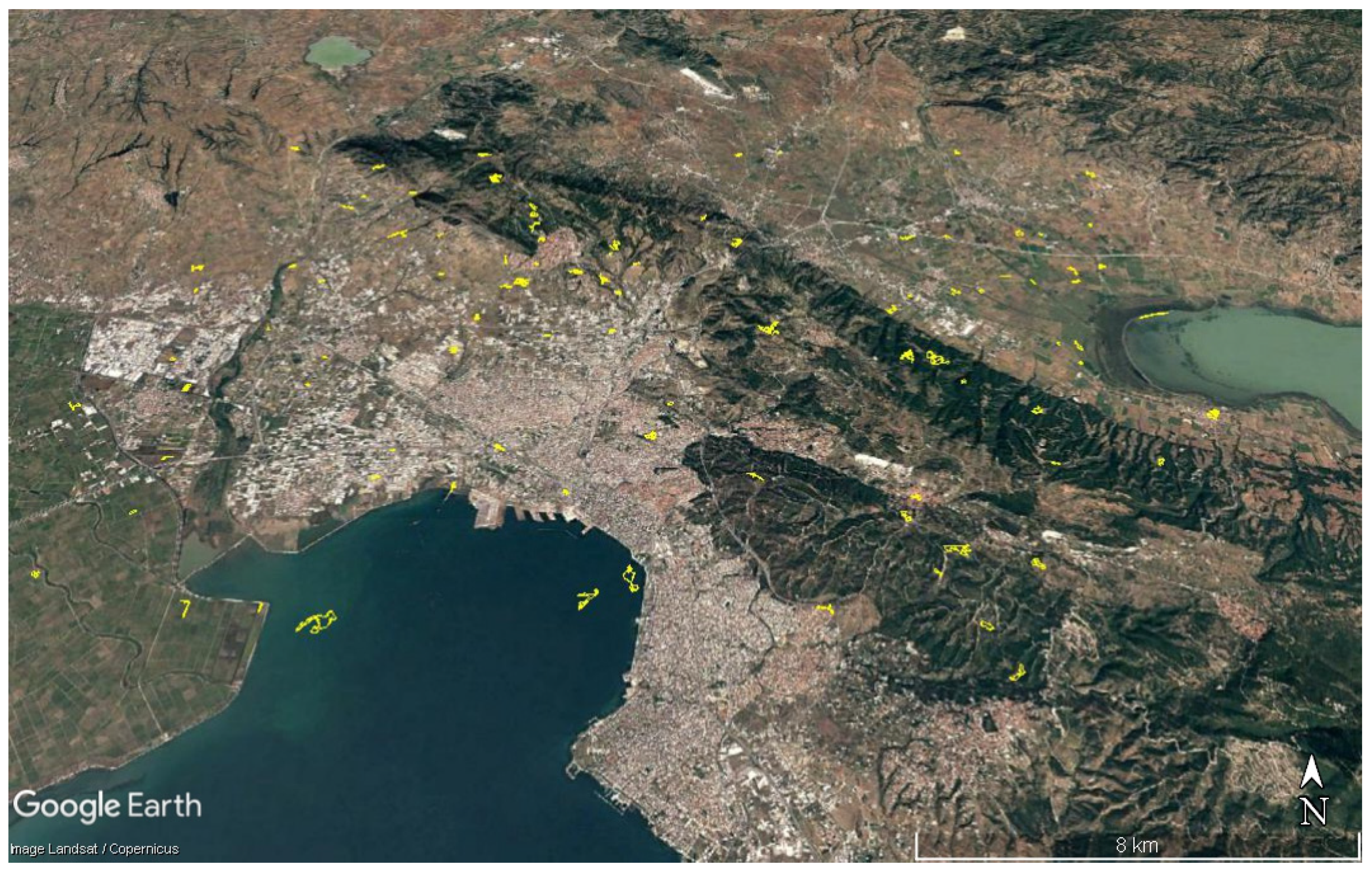
3.1. Image Data

A subset of 600 km² (20 × 30 km) extracted from a Sentinel-2 image scene, acquired on 28 June 2017 as a bottom of atmosphere (BOA) reflectance matrix (LA2 mode) and projected into the WGS84 reference system, UTM zone N34, was used for the experimentation. The image was cloud-free and of excellent quality. The dataset was downloaded from the Copernicus Open Access Hub portal [29].

Sentinel-2 is ready-to-use, high-resolution imagery, available for free from the European Space Agency (ESA). Its MultiSpectral Instrument (MSI) carries 13 spectral bands ranging from the visible and near-infrared to the short-wave infrared wavelengths. The spatial resolution varies from 10 to 60 m, depending on the spectral band, with a 290 km field of view [29].

The unique combination of high spatial resolution, wide field of view and broad spectral coverage, together with their free availability as ready-to-use products in an atmospherically corrected reflectance mode, has opened up a new window in operational land use mapping [30]. The spectral bands of Sentinel-2 are specified as follows (in brackets the pixel size of every band, in meters; wavelengths at the center of the bandwidth, in nm): B1(60)—443; B2(10)—490; B3(10)—560; B4(10)—665; B5(20)—705; B6(20)—740; B7(20)—783; B8(10)—842; B8a(20)—865; B9(60)—940; B10(60)—1375; B11(20)—1610; B12(20)—2190.

The image subset covers urban and industrial areas, agricultural fields, forests, shrubs, meadows, and water bodies. In terms of CORINE Land Cover nomenclature, the study area is shared between 24 different 3rd-level categories.

The 60 m resolution bands (B1, B9, and B10, dedicated to capturing coastal aerosols, water vapors, and cirrus, respectively) were removed from the original Sentinel-2 dataset. Additionally, the 20 m resolution bands (B5, B6, B7, B8a, B11, and B12) were resampled into 10 m bands to form finally a 10-m resolution image composite of 10 spectral bands (Figure 1).

3.2. Functional Scales

As explained in the Section 2.1, the functional scales of a specific environment can be detected with image segmentation, as the size of the objects corresponding to the optimal segmentation scales are considered equivalent to the functional scales.

The optimal segmentation scales in the current experimental study were taken from a relevant study with the same Sentinel-2 subset conducted by Karydas (2020) [26]. In that study, a series of systematic segmentations was conducted using the Fractal Net Evolution Assessment (FNEA) algorithm with the color to shape parameter set to 9/1, while the compactness to smoothness parameter was set to 5/5. Such values are suggested when the dataset is unknown prior to the main analysis and a trial-and-error approach is used for the segmentation [31].

Finally, five optimal segmentation scales (in terms of scale factor, f_n) were detected for the subset: 5, 9, 16, 36, and 75. The mean object sizes and thus their equivalent functional scales corresponding to each of these segmentation scales were 203, 507, 1243, 4401, and 13,821 m², respectively (Figure 2).

As an indicative segmentation evaluation, the objects of the 75 scale (the largest among the optimum ones) were tested by an independent interpreter on Google Earth maps (Figure 3). The assessment was based on the purity (or internal homogeneity) of each object as regards containing a single surface material, e.g., concrete, soil, specific patterns of vegetation (high, low, dense, sparse, etc.), water, and so on.

Thus, every object was assigned a value between 50% and 100% according to the portion of the dominating land cover. For example, an object containing only soil (such as a bare agricultural field) was judged as 100% pure, whereas an object covered mainly by concrete (such as part of a village including though some vegetated yards) was judged, e.g., as 70% pure if one of the two components (concrete or vegetation) covered 70% of the object’s surface (Figure 4).

Purity was also assessed with regard to the shape of the objects; for example, when linear features, such as streets or drainage canals, were mixed with regularly shaped objects (e.g., a field or a construction), the purity value was assigned as the minimum (i.e., 50%). High values of purity (or internal homogeneity) and the easy discrimination of linear features (as separate objects) favor successful classification.

3.3. Classification Process

In this experimentation, the geographic scale (600 km²) and the observation scale (or resolution, 10 m) were predefined, as a Sentinel-2 image subset was selected for the classification. By entering the functional scales (indicated by the image segmentation of the subset) in the UST scale calculator, as well as the other computed scale parameters and constants, the conditions were checked and found to be met (“OK” notifications), while the minimum mapping unit per functional scale were also estimated (

Table 2. The scale calculator for the Sentinel-2 image subset and conditions running for Level-1 segmentation (data from Karydas 2020).

Geographic Scale	Observation Scale	Functional Scale						Cartographic Scale
Image size (m2)	Pixel (m)	Equation (2)
600,000,000	10.00	Min mean feature size						Equation (3)		Rule of thumb
Image side (m)	Surface (m2)	8.0		Radius (m)				1/	16,081	0.0005
24,495	100.00	203		Surface (m2)				Nominal scale	15,000	Condition-3
		Max number of objects								Nominal scale > 1
Condition-2	Condition-1	2,970,297								OK
Min. no. of objects	Min. object size/pixel			Equation (1)	Segmentation process			Minimum mapping units
>1	>1	Level	Integer(sn)	sn	fn	a	b	Side (m)	Radius (m)	Cartographic scale
43,409	2.03	1	203	202.7	5	16.48	1.5592	14.2	8.0	16,081
OK	OK	2	507	506.8	9	16.48	1.5592	22.5	12.7	25,414
		3	1243	1242.9	16	16.48	1.5592	35.3	19.9	39,792
		4	4401	4400.9	36	16.48	1.5592	66.3	37.4	74,876
		5	13,822	13,821.4	75	16.48	1.5592	117.6	66.3	132,694

The background color, font color, bold and italic allow visual grouping of concepts/cells into categories.

).

The maximum likelihood (ML) method was applied with ESRI ArcGIS program, one per segmentation level. ML implements a classification of all pixels in a multispectral image, by assigning each pixel to the class to which it has the highest probability of belonging [32]. The probabilities are computed from each class’s distribution of pixel values, derived from the training samples.

The exact process of the classification of the optimally segmented Sentinel-2 image was as follows:

• In ArcMap, a set of 100 random points was created for classification training purposes and another similar one for testing purposes;
• From every optimal segmentation layer, the objects containing training random points were selected (i.e., 100 objects per scale). As a result, 5 polygon-type training layers were created;
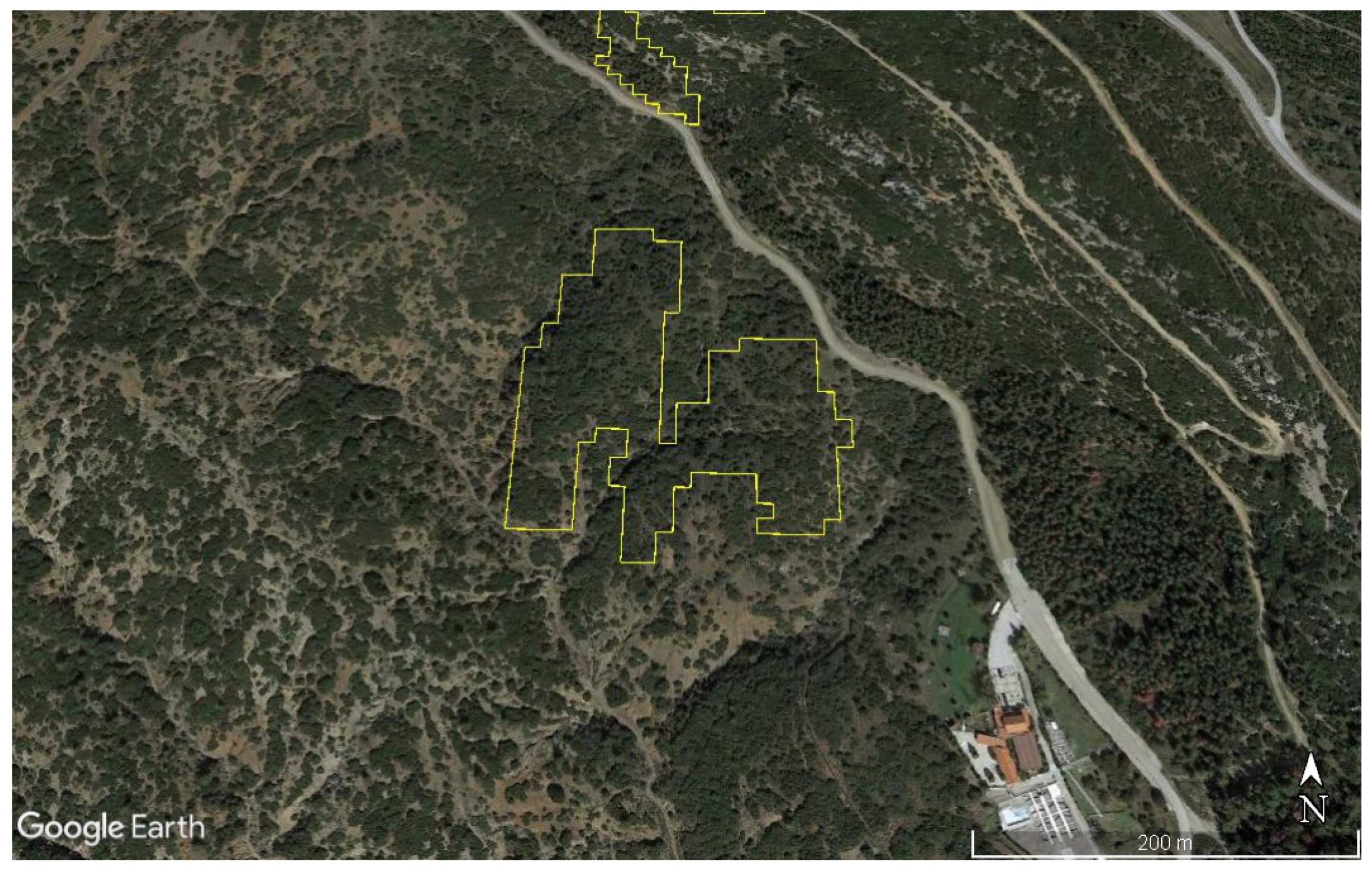
• The training layers were transferred to the Google Earth application (GE) and were updated with land cover information by an independent interpreter using the most contemporary GE background to the Sentinel-2 image (i.e., the closest possible to 28 June 2017). Interpretation was based on visual assessment judging from the dominant land cover/use within every object;
• Using the land cover information of the training samples, the Sentinel-2 image underwent pixel-based supervised classification using the ML algorithm;
• The class information was transferred to the testing objects (using a majority filter) for every layer. Thus, 5 test layers were created;
• The test layers were transferred to the Google Earth application, where they were assessed visually object by object by an independent interpreter;
• The updated test layers were transferred back to ArcMap, to calculate the accuracy figures.

The classification nomenclature was defined per each segmentation level separately. Thus, different classes were identified for every level according to the particularities of the meaningful objects recognized at that level, and more specifically:

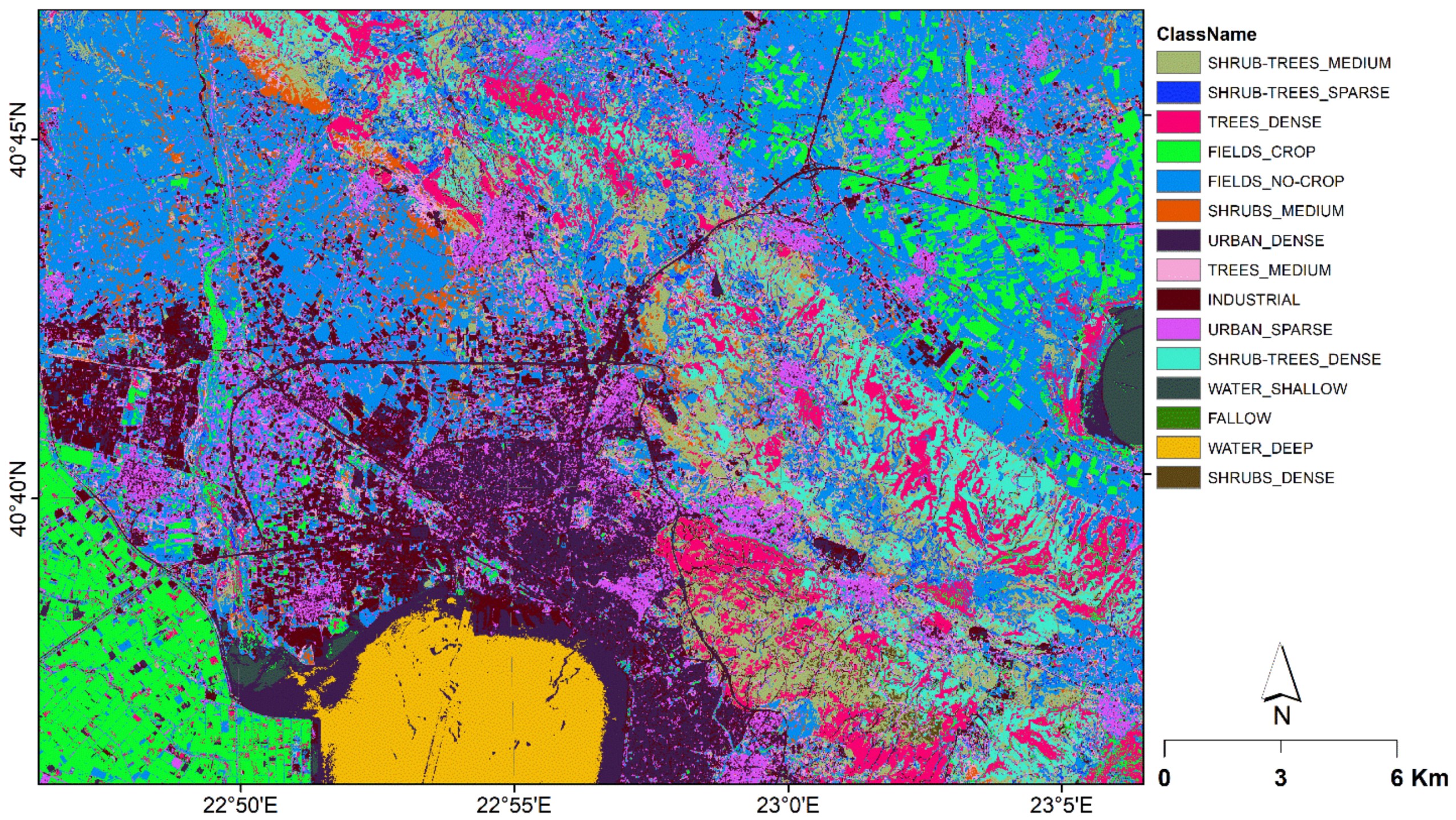
• At the 75-scale segmentation level, i.e., the largest among the optimum scales, a set of 15 different land cover/use classes was identified in the study area. The mean size of the objects at this level was 18,482 m², with the minimum of 1100 m² and maximum of 229,700 m². The urban environment was categorized into sparse and dense, while industrial environments were taken independently from other built up classes. Agricultural fields were characterized either as cultivated at the time of assessment or non-cultivated. Natural vegetation classes were distinguished into sparse, medium, or dense shrub, shrub trees, or tree compositions. Fallow land and water (divided into shallow and deep) were the remaining classes;
• At the 5-scale segmentation level, i.e., the smallest among the optimum scales, the mean size of the objects was 152 m², ranging from 100 m² to 1642 m². At this level, two different nomenclature schemes were tested:

  ◦

  One detailed scheme with a set of 55 classes, in accordance with the real complexity of the studied environment;

  ◦

  One simplified scheme, after grouping the detailed classes into more generalized ones (7 classes).

• For the rest of the optimal segmentation scales (9, 16, and 36), similar approaches to that of the 75-scale level were followed regarding nomenclature, with the number of classes ranging from 7 up to 11;
• In order to broaden the range of possible functional scales (beyond those suggested by the optimal ones), another two classifications were also attempted, one on the 139-scale and one on the 255-scale of segmentation. These scales, although indicated by the optimal scale detection method of Karydas (2020) [26], were rejected initially, as they did not meet the null-number condition of the method;
• In the 139-scale classification, classes containing only one sample were removed, and as a result, the classes were simplified (leaving 11 from the original class of 15 classes). In the new scheme, there were some classes that had not been identified on the 75-scale classification (e.g., Grassland). Finally, 9 out of the 100 samples were indicated as mixed classes, to a degree that was not possible to assess. This could be attributed to the fact that on this scale, objects are generally much larger than the previous scales.

4. Results and Discussion

The purity of the objects at the indicative 75-scale segmentation level (after assessment by an independent interpreter, see Section 3.2) was found to be 90.35% on average, with a standard deviation of 13.9%, and thus a coefficient of variation of 15.4%; 51 objects were found with 100% purity. These results indicate the very high internal homogeneity (purity) of the objects, which in turn creates a good basis for successful classification.

The classification process on the 75-scale resulted in an overall accuracy of 70% and producer’s and user’s accuracies ranging from 0 to 100% (

Table 3. The classification results of the Sentinel-2 subset of the 75-scale segmentation level.

No	Class for Scale Factor 75	Producer’s Accuracy (%)	User’s Accuracy (%)
1	Urban_Sparse	77.8	87.5
2	Urban_Dense	28.6	100.0
3	Industrial	71.4	45.5
4	Fields_Cultivation	58.3	70.0
5	Fields_No-Cultivation	90.3	73.7
6	Shrubs_Medium	0.0	N/A *
7	Shrubs_Dense	N/A	N/A
8	Shrub Trees_Sparse	100.0	50.0
9	Shrub Trees_Medium	50.0	71.4
10	Shrub Trees_Dense	77.8	77.8
11	Trees_Medium	0.0	N/A
12	Trees_Dense	62.5	71.4
13	Fallow Land	N/A	0.0
14	Water_Shallow	100.0	100.0
15	Water_Deep	100.0	66.7

* N/A stands for predefined classes not found in the classified image.

, Figure 5). According to Table 2, the cartographic scale corresponding to this level was 1:135,000, while the minimum mapping unit was approximately 1.3 ha.

Some of the disagreements of the classified image of the 75-scale segmentation with the reference data (collected from Google Earth) could be attributed to the temporal divergence between the two datasets; for example, an agricultural field might be cultivated during the period of Sentinel-2 image acquisition and be bare or cropped on the date of the Google Earth image background acquisition.

Unlike the 75-scale classification, the 5-scale classifications (i.e., both the detailed and the simplified schemes) failed completely to catch up with the true land cover/use patterns in the study area. This became obvious visually in both cases, and was enforced by the fact that only 11 out of 55 classes in the detailed classification scheme were represent in the classified image. Similarly, the intermediate scales (9, 16, and 36) failed to provide a convincing classified image. Thus, quantitative accuracy assessment was not attempted for any of these classifications.

The classification results on the 139-scale segmentation level resulted in an overall accuracy of 59.3% and producer’s and user’s accuracies ranging from 0 to 100% (

Table 4. The classification results of Sentinel-2 on the 139-scale segmentation.

No	Class for Scale Factor 138	Producer’s Accuracy (%)	User’s Accuracy (%)
1	Urban	100.0	100.0
2	Industrial	87.5	100.0
3	Fields	89.7	57.8
4	Shrubs_Sparse	11.8	33.3
5	Shrubs_Medium	0.0	0.0
6	Shrubs_Dense	71.4	55.6
7	Grassland	50.0	100.0
8	Forest Trees	0.0	0.0
9	Fallow Land	66.7	50.0
10	Water_Shallow	N/A	0.0
11	Water_Deep	100.0	100.0

, Figure 6). According to Table 2, the cartographic scale corresponding to this level was 1:215,000, while the minimum mapping unit was approximately 3.6 ha.

In some cases, the classes were not adequately represented (such as in the 16- and 36-scale classifications), and as a result, these classifications failed completely. It was also noticed that on the 5-scale classification, training the samples was more difficult than on larger scales, as the objects, although very small, contained different land features to a large degree. Thus, the judgement of the land cover captured by the training objects was very ambiguous, resulting in very uncertain outputs. In such cases, a solution could be to follow a fuzzy classification methodology.

An obvious question rising from the resulting low accuracies is “why does an optimal segmentation not lead necessarily to acceptable classification outputs?” However, the outputs of any image classification process are affected by several parameters, either controlled or uncontrolled, and in practice, the potential combinations of nomenclatures and hierarchies with classifiers, sampling methods or rules, use of pixels or objects, and with the scale or scales of implementation are infinite, and thus impossible to compare and assess beyond the scope of specific classification.

5. Conclusions

Building upon previous knowledge about scale, the Unified Scale Theorem (UST) manages to link the four concepts of scale into a single mathematical formulation, and thus confirm the basic hypothesis of this research. In addition to that, a scale calculator is provided as an interactive Excel spreadsheet to facilitate image interpreters in selecting scales for classification purposes in a holistic way.

UST is justified for classification as a theorem because of the following [33]:

• Its core part (i.e., the segmentation process adapted from Karydas 2020) is a proven theorem;
• It is supported by an axiom, namely the rule of thumb for human eye distinction capability;
• It contains an obvious statement, namely the equivalence of mean object size at a segmentation level with the functional scale at that level;
• It is confined by limitations (the three predefined conditions);
• It is verified by experimentation.

The fully numerical character of UST promotes objectivity and rapidity in optimal scale selection for image classification. Even more importantly, classification accuracy potential increases, considering that segmentation purity, which is a prerequisite for successful classifications, was found experimentally to be excellent (over 90% in the conducted study).

UST can be implemented in a twofold way: either towards a “feature-based classification”, in terms of using spatial features’ properties for defining the classes, or towards a “nomenclature-based classification”, whereby spatial features are forced to comply with predefined classes. With the former approach, which can be called “Special UST”, the observation scale (resolution) is known in advance, whereas functional scales are the unknown parameters. This approach was employed in the current work through the conducted experimentation.

With the latter approach (not focused on here), which can be called “General UST”, functional scales are the known parameters (derived from the scope of the classification project), whereas observation scales (resolutions) are the unknown parameters. Future work will focus on experimenting with different image data types and various classification nomenclatures, thus allowing the generalization of the Unified Scale Theorem.

The overall investigation presented in this study sheds light on the self-similar hierarchy theory in the field of geosciences, and introduces fractal geometry to image classification theory. It also provides a new basis for resolving the Modifiable Areal Unit Problem (MAUP), a known problem in geography, stemming from the use of different data sources, zonings, or data aggregation methods [34].

References

- Goodchild, M.F. Metrics of scale in remote sensing and GIS. Int. J. Appl. Earth Obs. Geoinf. 2001, 3, 114–120. [Google Scholar] [CrossRef]
- Levin, S.A. The problem of pattern and scale in ecology. Ecology 1992, 73, 1943–1967. [Google Scholar] [CrossRef]
- Marceau, D.J.; Hay, G.J. Remote Sensing Contributions to the Scale Issue. Can. J. Remote Sens. 1999, 25, 357–366. [Google Scholar] [CrossRef]
- Zahra, D.; Blaschke, T. Scale matters: A survey of the concepts of scale used in spatial disciplines. Eur. J. Remote Sens. 2019, 52, 419–434. [Google Scholar]
- Lillesand, T.M.; Kiefer, R.W. Remote Sensing and Image Interpretation; John Wiley and Sons, Inc.: New York, NY, USA, 1994; Chapter 7; 750p. [Google Scholar]
- Lu, D.; Weng, Q. A survey of image classification methods and techniques for improving classification performance. Int. J. Remote Sens. 2007, 28, 823–870. [Google Scholar] [CrossRef]
- Dey, V.; Zhang, Y.; Zhong, M. A review on image segmentation techniques with Remote Sensing perspective. In Proceedings of the ISPRS TC VII Symposium—100 Years ISPRS, Vienna, Austria, 5–7 July 2010; Wagner, W., Székely, B., Eds.; IAPRS: Vienna, Austria, 2010; Volume XXXVIII. Part 7A. [Google Scholar]
- Haralick, R.M.; Shapiro, L.G. Image segmentation techniques. Comput. Vis. Graph. Image Process. 1985, 29, 100–132. [Google Scholar] [CrossRef]
- Karydas, C.G.; Gitas, I.Z. Development of an IKONOS image classification rule-set for multi-scale mapping of Mediterranean rural landscapes. Int. J. Remote Sens. 2011, 32, 9261–9277. [Google Scholar] [CrossRef]
- Dragut, L.; Csillik, O.; Eisank, C.; Tiede, D. Automated parameterisation for multi-scale image segmentation on multiple layers. ISPRS J. Photogramm. Remote Sens. 2014, 88, 119–127. [Google Scholar] [CrossRef] [Green Version]
- Janowski, L.; Tylmann, K.; Trzcinska, K.; Rudowski, S.; Tegowski, J. Exploration of Glacial Landforms by Object-Based Image Analysis and Spectral Parameters of Digital Elevation Model. IEEE Trans. Geosci. Remote Sens. 2021, 1–17. [Google Scholar] [CrossRef]
- Parish, E.J.; Duraisamy, K. A Unified Framework for Multiscale Modeling Using Mori–Zwanzig and the Variational Multiscale Method. arXiv 2018, arXiv:1712.09669. [Google Scholar]
- Jiang, B.; Yin, J. Ht-Index for Quantifying the Fractal or Scaling Structure of Geographic Features. Ann. Assoc. Am. Geogr. 2014, 104, 530–540. [Google Scholar] [CrossRef]
- Lam, N.S.-N.; Quattrochi, D. On the Issues of Scale, Resolution, and Fractal Analysis in the Mapping Sciences. Trans. Am. Geophys. Union 1992, 2, 638–693. [Google Scholar] [CrossRef]
- Sun, W.; Xu, G.; Gong, P.; Liang, S. Fractal analysis of remotely sensed images: A review of methods and applications. Int. J. Remote Sens. 2006, 27, 4963–4990. [Google Scholar] [CrossRef]
- Martins, M.D.; Laaha, S.; Freiberger, E.M.; Choi, S.; Fitch, W.T. How children perceive fractals: Hierarchical self-similarity and cognitive development. Cognition 2014, 133, 10–24. [Google Scholar] [CrossRef] [Green Version]
- Hay, G.J.; Marceau, D.J.; Dube, P.; Bouchard, A. A Multiscale Framework for Landscape Analysis: Object-Specific Analysis and Upscaling. Landsc. Ecol. 2001, 16, 471–490. [Google Scholar] [CrossRef]
- Lam, N.S.-N.; Qiu, H.L.; Quattrochi, D.A.; Emerson, C.W. An evaluation of fractal methods for characterizing image complexity. Cartogr. Geogr. Inf. Sci. 2002, 29, 25–35. [Google Scholar] [CrossRef]
- Mandelbrot, B. The Fractal Geometry of Nature; W. H. Freeman and Co.: New York, NY, USA, 1982. [Google Scholar]
- Roy, A.G.; Gravel, G.; Gauthier, C. Measuring the dimension of surfaces: A review and appraisal of different methods. In Proceedings of the Eighth International Symposium on Computer-Assisted Cartography(Auto–Carto8), Baltimore, MD, USA, 29 March–3 April 1987; pp. 68–77. [Google Scholar]
- Tate, N.J. Estimating the fractal dimension of synthetic topographic surfaces. Comput. Geosci. 1998, 24, 325–334. [Google Scholar] [CrossRef]
- Sun, W. Three new implementations of the triangular prism method for computing the fractal dimension of remote sensing images. Photogramm. Eng. Remote Sens. 2005, 72, 373–382. [Google Scholar] [CrossRef]
- Husain, A.; Reddy, J.; Bisht, D.; Sajid, M. Fractal dimension of coastline of Australia. Sci. Rep. 2021, 11, 6304. [Google Scholar] [CrossRef]
- Berke, J. Using Spectral Fractal Dimension in Image Classification. In Innovations and Advances in Computer Sciences and Engineering; Sobh, T., Ed.; Springer: Dordrecht, The Netherlands, 2010. [Google Scholar]
- Unified Field Theory, Wikipedia. Available online: https://en.wikipedia.org/wiki/Unified_field_theory (accessed on 21 August 2021).
- Karydas, C.G. Optimization of multi-scale segmentation of satellite imagery using fractal geometry. Int. J. Remote Sens. 2020, 41, 2905–2933. [Google Scholar] [CrossRef]
- Karydas, C.; Jiang, B. Scale Optimization in Topographic and Hydrographic Feature Mapping Using Fractal Analysis. ISPRS Int. J. Geo-Inf. 2020, 9, 631. [Google Scholar] [CrossRef]
- Bobick, A.; Bolles, R. The representation space paradigm of concurrent evolving object descriptions. IEEE Trans. Pattern Anal. Mach. Intell. 1992, 14, 146–156. [Google Scholar] [CrossRef]
- European Space Agency (ESA). Available online: https://www.esa.int/ESA (accessed on 5 August 2019).
- Torma, M.; Hatunen, S.; Harma, P.; Jarvenpaa, E. Sentinel-2 Images and Finnish Corine Land Cover Classification. In Proceedings of the 1st ESA Sentinel-2 Preparatory Symposium, Frascati, Italy, 23–27 April 2012. [Google Scholar]
- Benz, U.C.; Hofmann, P.; Willhauck, G.; Lingenfelder, I.; Heynen, M. Multi-resolution, object-oriented fuzzy analysis of remote sensing data for GIS-ready information. ISPRS J. Photogramm. Remote Sens. 2004, 58, 239–258. [Google Scholar] [CrossRef]
- ArcMap Documentation. Available online: https://desktop.arcgis.com/en/arcmap/10.3/tools/spatial-analyst-toolbox/how-maximum-likelihood-classification-works.htm (accessed on 18 August 2021).
- The Definitive Glossary of Higher Mathematical Jargon. Available online: https://mathvault.ca/math-glossary/#theorem (accessed on 11 September 2021).
- Ratcliffe, J.H.; McCullagh, M.J. Hotbeds of Crime and the Search for Spatial Accuracy. J. Geogr. Syst. 1999, 1, 385–398. [Google Scholar] [CrossRef]