Article

Sinc Based Inverse Laplace Transforms, Mittag-Leffler Functions and Their Approximation for Fractional Calculus

1
Mathematics Department, German University in Cairo, New Cairo City, Egypt
2
Institute of Mathematical Physics, Ulm University, 89081 Ulm, Germany
Fractal Fract. 2021, 5(2), 43; https://doi.org/10.3390/fractalfract5020043
Submission received: 14 April 2021 / Revised: 29 April 2021 / Accepted: 6 May 2021 / Published: 10 May 2021
(This article belongs to the Special Issue Fractal Functions and Applications)

Abstract

:
We shall discuss three methods of inverse Laplace transforms. A Sinc-Thiele approximation, a pure Sinc, and a Sinc-Gaussian based method. The two last Sinc related methods are exact methods of inverse Laplace transforms which allow us a numerical approximation using Sinc methods. The inverse Laplace transform converges exponentially and does not use Bromwich contours for computations. We apply the three methods to Mittag-Leffler functions incorporating one, two, and three parameters. The three parameter Mittag-Leffler function represents Prabhakar’s function. The exact Sinc methods are used to solve fractional differential equations of constant and variable differentiation order.

1. Introduction

In the present paper, we present three methods for carrying out the numerical inversion of the Laplace transform [1]. The methods are all based on Sinc approximations of rational expressions via Thiele’s continued fraction approximation (STh) [2], indefinite integral approximations based on a Sinc basis [3], and indefinite integral approximations based on a Sinc-Gaussian (SG) basis [4]. The three methods avoid Bromwich contours requiring a special parameter adaptation on each time step [5,6,7,8,9]. The motivation behind avoiding Bromwich contours is to represent numerically generalized functions and provide a practical method for computing inverse Laplace transforms. Among the generalized functions, we aim at Mittag-Leffler (ML) functions, and especially Prabhakar functions among them. ML functions are frequently used in fractional calculus [10,11,12,13,14]. For an overview and detailed discussion of theoretical properties and applications of the Mittag-Leffler functions, see the recent book by Gorenflo et al. [14] and Kilbas [15]. Mittag-Leffler a Swedish mathematician introduced this function at the beginning of the last century [16] to generalize the exponential function by a parameter α :
E α ( z ) = k = 0 z k Γ ( α k + 1 ) with α C , ( α ) > 0 , and z C .
Three years later, Wiman [17] extended the one-parameter function to a two-parameter function also defined as an infinite series using gamma functions Γ ( x ) to replace the factorial in its definition:
E α , β ( z ) = k = 0 z k Γ ( α k + β ) with α , β C , ( α ) > 0 , and z C .
In 1971, the Indian mathematician Prabhakar [18] proposed another generalization to three parameters, i.e.,
E α , β γ ( z ) = 1 Γ ( γ ) k = 0 Γ ( γ + k ) z k Γ ( k + 1 ) Γ ( α k + β ) with α , β , γ C , ( α ) > 0 , and z C .
Comparing these series definitions of higher parameter ML functions, it is obvious that all of them are generalizations of the exponential and, thus, include the exponential function as a limiting case. There are many other ML functions in use with larger numbers of parameters especially in fractional calculus; for a detailed discussion of these types of functions, see Reference [15]. We shall restrict our examinations of the numerical representation to the above three variants because, currently, they are the most frequently used in fractional calculus. However, the higher-order ones can be included in our approach in a straightforward way if needed. One common property of the ML functions as stated above is the Laplace representation G ( s ) as a transfer function instead of the infinite series. The series representation is not an efficient option for numerical computations because the convergence of the series is sometimes restricted to | z | < 1 , the sequence of the terms in the series do not decrease monotonically [19], and the numerical evaluation of the Γ function is usually limited to a restricted magnitude of the argument if single or double precision is used in computations. For this reason, we use the Laplace route to avoid such kinds of convergence limiting problems.
That is, if R + denotes the interval ( 0 , ) , we obtain accurate approximations to f defined on R + by
L f = G ( s ) ,
where G the transfer function is given on R + . The Laplace transform L f is defined by
( L f ) ( s ) = 0 e s t f ( t ) dt .
The Laplace transform occurs frequently in the applications of mathematics, physics, engineering and is a major tool today in fractional analysis [13,20], especially in the representation of special functions. We will use this technique to numerically represent functions, like the ML functions needed in practical applications of relaxation processes. However, one of the major problems of the Laplace transform is and especially its inverse, contrary to Fourier transform, is that there is no universal method of inverting the Laplace transform. In applications, such as fractional calculus, G is frequently known on R + , and the use of the Bromwich inversion formula [21]
f ( t ) = 1 2 π i σ i σ + i e s t G ( s ) ds
is, therefore, not analytically feasible in many cases. Recently, the Bromwich inversion formula was used in connection with Talbot’s idea to replace the Bromwich contour C C by a simplified contour in C [5,6,7,8]. However, it turned out that a special tuning of the parameters in the parametric representation of the contour is needed to achieve trust-able results. The lack of universal methods for inverting the Laplace transforms stems from the fact that the space of functions f for which L f exists is simply speaking too big. We immediately restrict this space by assuming that f L 2 R + , which implies that G L 2 R + . In applications, it is generally possible to achieve this criterion via elementary manipulations [22]. An excellent summary of other methods for inverting the Laplace transform is contained in Reference [23]. Furthermore, the methods summarized in Reference [23] are tested on several functions. While the tests in Reference [23] are interesting, the criteria of testing do not restrict the space of functions; thus, it is possible to write down test functions for which any one of the methods does extremely well, while all of the others fail miserably. A variety of other methods are discussed in Reference [20] and references in Reference [22].
The connection between the Laplace transform G ( s ) and the function f ( t ) is easily recognized if we recap the physical background in dielectric relaxation processes. Let us assume for simplicity of the discussion that the orientation polarization P or is related to the alignment of dipoles in the electric field, whereby the permanent dipoles are rigidly connected to the geometry of the molecule. Thus, the time for complete development of P or is coupled to the rotational mobility of the molecules. This, in turn, is a variable that is closely related to the viscosity η of the substance. The simplest approach to describe a temporal law for P or ( t ) is incorporated in the idea that, after switching on an electric field, E ( t ) = E 0 for t > 0 , the change dP or dt depends linearly on P or ( t ) , which is known as Debye relaxation of dielectrics [24], resulting in the celebrated relaxation equation
dP or dt = τ 1 P or .
The solution of the initial value problem (7) is given by the exponential function P or ( t ) = P or ( 0 ) exp ( t / τ ) with τ the relaxation time. More interestingly, the Laplace representation of this relation which, in terms of a standard relaxation function χ ( t ) , reads
s χ ^ ( s ) = 1 τ χ ^ ( s ) + χ ( 0 ) ,
or
χ ^ ( s ) = χ ( 0 ) s + τ 1 .
Delivering immediately the time dependent solution χ ( t ) = χ ( 0 ) exp ( t / τ ) using the inverse Laplace transform. A canonical fractionalization of the standard relaxation Equation (7) in terms of χ ( t ) result to
D α χ ( t ) = τ α χ ( t ) + χ 0 t α Γ ( 1 α ) ,
using the initial condition χ ( 0 ) = χ 0 ; here, D α represents the Riemann-Liouville fractional derivative. Since Equation (10) is a linear equation, we can get the Laplace transform of this equation including the initial condition χ 0 as
χ ^ ( s ) = χ 0 s α 1 s α + τ α .
Inversion of the transfer function by involving a Mellin transform results to the time dependent solution χ ( t ) = χ 0 E α ( t / τ ) α [25], where E α ( z ) is the one parameter ML function E α ( z ) defined in classical terms as an infinite series by Equation (1). The comparison with the exponential function exp ( z ) = k = 0 z k Γ ( k + 1 ) reveals that E α ( z ) is in fact a generalization of the exponential function using the fractional parameter α restricted to 0 < α < 1 .
Another type of fractional relaxation equation which changes the initial decay of the process by an additional fractional exponent β is given by the following two-parameter equation
D α χ ( t ) = τ α χ ( t ) + χ 0 t β α 1 Γ ( β α ) .
Applying the same procedure as before, we get the transfer function representation as
χ ^ ( s ) = χ 0 s α β s α + τ α .
After inverting the Laplace transform by using the Mellin transform [12,25,26], we gain the two-parameter ML function
χ ( t ) = χ 0 t β 1 E α , β ( t / τ ) α .
Again, the comparison with exp ( z ) and E α ( z ) reveals that E α , β ( z ) is a generalization of the exponential function. We could continue in this way by adding additional parameters to get generalized rational expressions in Laplace space resulting in generalized functions of the exponential. We will get back to this idea in a moment. However, Prabhakar followed another route which is based on the following Laplace representation of a function (see. Kilbas et al. [15]) using multiplications instead of additions in the parameter set α , β , and γ as follows:
χ ^ ( s ) = χ 0 s γ α β s α + τ α γ ,
delivering a three parameter generalization of the exponential function as
χ ( t ) = χ 0 t β 1 E α , β γ ( t / τ ) α ,
with
E α , β γ ( z ) = k = 0 ( γ ) k z k Γ ( k + 1 ) Γ ( α k + β ) , α , β , γ C , ( α ) > 0 , z C ,
where ( γ ) k = Γ ( γ + k ) / Γ ( γ ) is the Pochhammer symbol, and Γ ( z ) denotes the Euler gamma function. Note that Prabhakar’s function is an entire function of order ρ = 1 / ( α ) and type σ = 1 [14]. The above Prabhakar model can be reduced to a Riemann-Liouville fractional integral equation of relaxation type [27]. In this framework of Laplace transforms, we can introduce generalized transfer functions G ( s ) in the Laplace space incorporating many parameters combined in different ways.
Such an approach was proposed in the field of electronic filter design, such as low-pass, high-pass, and bandpass filters, including the construction of a rational function that satisfies the desired specifications for cutoff frequencies, pass-band gain, transition bandwidth, and stop-band attenuation. Recently, these rational approximations were extended to fractal filters improving the design methodology in some direction. Following Podlubny [28], a fractional-order control system can be described by a fractional differential equation of the form:
a n D α n χ ( t ) + a n 1 D α n 1 χ ( t ) + + a 0 D α 0 χ ( t ) =
b m D β m χ ( t ) + b m 1 D β m 1 χ ( t ) + + b 0 D β 0 χ ( t )
or by an equivalent continuous transfer function
G ( s ) = b m s β m + b m 1 s β m 1 + + b 0 s β 0 a n s α n + a n 1 s α n 1 + + a 0 s α 0 .
The use of the continuous transfer function is today the standard approach to design filters. The transfer function uses fractional exponents α i and β j to represent the fractional orders of the differential equations. The problem with this approach is that only in rare cases a direct inversion of the Laplace representation to the time domain is possible. One way to solve this problem was originally proposed by Roy; that is the transfer function G ( s ) with fractional exponents can be replaced by a rational approximation G ˜ ( s ) using natural number exponents [29]. Such kind of rational approximation G ˜ ( s ) can be generated by a Sinc point based Thiele algorithm (STh) [2,30]. Thiele’s algorithm converts a rational expression to a continued fraction representation which is related to a rational expression possessing exponents of natural numbers. Such kind of approximation will change of course the representation of the rational character of the transfer function but allows us to use a fraction with integer orders if we need to invert the Laplace transformation. The benefit here is that, for rational functions with integer powers, a well-known method by Heaviside exists, also called the partial fraction method, to invert a Laplace transform to a sum of exponential functions. This is in short how the method of numerical approximation of all the different transfer functions mentioned above can be transformed to the time domain with sufficient accuracy.
From a practical point of view of the STh approach, we gain a numerical representation of the function but miss the analytic properties if we are not able to compute the inverse Laplace transform analytically. In some cases, an analytic representation is possible via Mellin-Barns integrals delivering special function included in the class of Fox-H functions [11,13,15,26]. For our numerical computations, however, this is not a disadvantage if we are aware that the numerical results belong to this larger class of special functions which are representable by Mellin-Barns integrals. Given the ML function, we know that these functions belong to this class of Fox-H functions. The gain of the numerical inversion of the Laplace transform, however, is that, at least for practical work, we have access to the determining parameters of the function.
The paper is organized as follows: Section 2 introduces, in short, the methodology of Sinc methods. Section 3 discusses some applications and error estimations. Section 4 summarizes the work and gives some perspectives for additional work.

2. Sinc Methods of Approximation

This section discusses the used methods of approximation for the two sets of basis functions. First, the approximation of functions is introduced defining the terms and notion. The second part deals with approximations of indefinite integrals. Based on these definitions, we introduce the approximation of inverse Laplace transform in the next step. We use the properties of Sinc functions allowing a stable and accurate approximation based on Sinc points [31]. The following subsections introduce the basic ideas and concepts. For a detailed representation, we refer to References [30,32,33].
In their paper, Schmeisser and Stenger proved that it is beneficial to use in Sinc approximations a Gaussian multiplier [4]. The idea of using a Gauss multiplier in connection with Sinc approximations is a subject discussed in literature from an application point of view by Qian [34]. The group around Qian observed that a Gauss multiplier improves under some conditions the convergence of an approximation [35]. Schmeisser and Stenger verified this observation on a theoretical basis and proved an error formula possessing exponential convergence [4]. A similar approach was used by Butzer and Stens [36] to improve the convergence in a Sinc approximation in connection with the Whittaker-Kotelnikov-Shannon sampling theorem. The general multiplier used by Butzer and Stens is here replaced by a Gaussian. We note that the used multiplier function used by Butzer and Stens in the limit m is the same as the Gaussian for c 0 . It turned out that the approximation is useful not only to represent functions but can be also applied to integrals and integral equations, as well as to derivatives.
It is a well-known fact that numerical Laplace transform and especially its inversion is much more difficult than numerical integration. It turns out that numerical inverse Laplace transform based on Bromwich’s integral is influenced by several factors, like the choice of nodes, the method of integration used, the algorithmic representation, and the structure of the contour to mention only a few. In applications, it is sometimes required that a certain accuracy is achieved over a definite or semi-infinite interval, and specifically at the boundaries. It would be beneficial if the method is easy to implement, and the number of computing steps is minimized. In addition, from the mathematical point of view, we may gain some insights if an ad hoc estimation of the error is possible. Such a set of requirements is, in most of the cases, not available; either one of the properties is missing, or the whole set of requirements cannot be satisfied by a specific method. We will discuss a new method that was mentioned in a basic form in an application to initial value problems [1]. Our new method uses the basic idea of collocating indefinite integrals in connection with the fundamental theorem of calculus. This allows us to approximate a basic relation using either a Sinc basis or a Sinc-Gaussian (SG) basis. Both approaches will be discussed and used in examples.
To put our results in perspective, we briefly discuss the basics of approximations using a Sinc-Gaussian basis, indefinite integrals, convolution integrals, and the inverse Laplace transform.

2.1. Sinc Basis

To start with, we first introduce some definitions and theorems allowing us to specify the space of functions, domains, and arcs for a Sinc approximation.
Definition 1.
Domain and Conditions.
Let D be a simply connected domain in the complex plane and z C having a boundary D . Let a and b denote two distinct points of D and ϕ denote a conformal map of D onto D d , where D d = { z C : | I m ( z ) | < d } , such that ϕ ( a ) = and ϕ ( b ) = . Let ψ = ϕ 1 denote the inverse conformal map, and let Γ be an arc defined by Γ = { z C : z = ψ ( x ) , x R } . Given ϕ, ψ, and a positive number h, let us set z k = ψ ( k h ) , k Z to be the Sinc points, let us also define ρ ( z ) = e ϕ ( z ) .
Note the Sinc points are an optimal choice of approximation points in the sense of Lebesgue measures for Sinc approximations [37].
Definition 2.
Function Space.
Let d ( 0 , π ) , and let the domains D and D d be given as in Definition 1. If d is a number such that d > d , and, if the function ϕ provides a conformal map of D onto D d , then D D . Let α and β denote positive numbers, and let L α , β ( D ) denote the family of functions u H o l ( D ) , for which there exists a positive constant c 1 such that, for all z D ,
| u ( z ) | c 1 | ρ ( z ) | α ( 1 + | ρ ( z ) | ) α + β .
Now, let the positive numbers α and β belong to ( 0 , 1 ] , and let M α , β ( D ) denote the family of all functions g H o l ( D ) , such that g ( a ) and g ( b ) are finite numbers, where g ( a ) = lim z a g ( z ) and g ( b ) = lim z b g ( z ) , and such that u L α , β ( D ) where
u ( z ) = g ( z ) g ( a ) + ρ ( z ) g ( b ) 1 + ρ ( z ) .
These definitions directly allow the formulation of an algorithm for a Sinc approximation. Let Z denote the set of all integers. Select positive integers N and M = [ β N / α ] so that m = M + N + 1 . The step length is determined by h = ( π d / ( β N ) ) 1 / 2 where α , β , and d are real parameters. In addition, assume there is a conformal map ϕ and its inverse ψ such that we can define Sinc points z j = ψ ( j h ) , j Z [38]. The following relations define the basis of a Sinc approximation:
Sin c ( z ) = sin ( π z ) π z .
The sifted Sinc is derived from relation (23) by translating the argument by integer steps of length h and applying the conformal map to the independent variable.
B ( k , h , c ) ( x ) = S ( k , h ) ( z ) if c = 0 S ( k , h , c ) ( z ) if c 0 ,
where S ( k , h ) ( z ) = sin ( π ( z / h k ) ) / ( π ( z / h k ) ) = Sin c ( z / h k ) represents the Sinc function and S ( k , h , c ) ( z ) = Sin c ( z / h k ) exp c ( z / h k ) 2 is the Sinc-Gaussian. The first type of approximation results to the representation
C h , M , N [ f ] ( z ) = k = M N f z k Sin c ϕ ( z ) h k ,
using the basis set of orthogonal functions
B S = { S ( k , h ) ϕ ( z ) } k = M N = { S ( k , h ) ϕ ( z ) } k = M N ,
where ϕ ( z ) is a conformal map. As discussed by Schmeisser and Stenger [4], a Sinc approximation of a function f can be given in connection with a Gaussian multiplier in the following representation:
C h , c , M , N [ f ] ( z ) = k = M N f z k Sin c ϕ ( z ) h k exp c ϕ ( z ) h k 2 ,
with c a constant, and ϕ denoting a conformal map. This type of approximation allows to represent a function f ( z ) on an arc Γ with an exponential decaying accuracy [4]. As demonstrated in Reference [4], the approximation works effective for analytic functions. The definition of the Sinc-Gaussian basis by
B S G = S ( k , h ) ϕ ( z ) exp c ϕ ( z ) k h h 2 k = M N = { S ( k , h , c ) ϕ ( z ) } k = M N
allows us to write the approximation in a compact form as
C h , c , M , N [ f ] ( z ) = k = M N f z k S ( k , h , c ) ϕ ( z ) .
The two approximations allow us to formulate the following theorem for Sinc approximations.
Theorem 1.
Sinc Approximation [38].
Let u L α , β ( D ) for α > 0 , β > 0 , and d as in Definition 2, take M = [β N/α], where [x] denotes the greatest integer in x, and then set m = M + N + 1 . If u M α , β ( D ) , and, if h = ( π d / ( β N ) ) 1 / 2 , then there exists a positive quantity, such that
f ( x ) C h , c , M , N [ f ] ( x ) = K 1 N 1 / 2 exp k 1 N 1 / 2 ,
using w k as basis functions (see (31)). Here, K 1 and k 1 are constants independent of N.
The proof of this theorem is given for the pure Sinc case in References [4,30] discusses the SG case. Note the choice h = ( π d / ( β N ) ) 1 / 2 is close to optimal for an approximation in the space M α , β ( D ) in the sense that the error bound in Theorem 1 cannot be appreciably improved regardless of the basis [38]. It is also optimal in the sense of the Lebesgue measure achieving an optimal value less than Chebyshev approximations [37].
Here, z k = ψ ( k h ) = ϕ 1 ( k h ) are the discrete points based on Sinc points k h . Note that the discrete shifting allows us to cover the approximation interval ( a , b ) in a dense way, while the conformal map is used to map the interval of approximation from an infinite range of values to a finite one. Using the Sinc basis, we can represent the basis functions as a piecewise-defined function w j ( z ) by
w j = 1 1 + ρ ( z ) k = M + 1 N 1 1 + e k h B ( k , h , c ) ϕ ( z ) j = M B ( k , h , c ) ϕ ( z ) j = M + 1 , , N 1 ρ ( z ) 1 + ρ ( z ) k = M N 1 e k h 1 + e k h B ( k , h , c ) ϕ ( z ) j = N ,
and c = 0 or c 0 , where ρ ( z ) = exp ( ϕ ( z ) ) . This form of the Sinc basis is chosen as to satisfy the interpolation at the boundaries. The basis functions defined in (31) suffice for purposes of uniform-norm approximation over ( a , b ) .
This notation allows us to define a row vector V m ( B ) of basis functions
V m ( B ) = w M , , w N ,
with w j defined as in (31). For a given vector V m ( u ) = u M , , u N T , we now introduce the dot product as an approximation of the function u ( z ) by
u ( z ) V m ( B ) . V m ( u ) = k = M N u k w k .
Based on this notation, we will introduce in the next few subsections the different integrals we need [32].

2.2. Indefinite Integral Approximation

In this section, we pose the question of how to approximate indefinite integrals on a sub-domain of R . The approximation will use our basis system introduced in Section 2.1. We will introduce two different approximations using Sinc and Sinc-Gaussian basis. It turns out that, for both basis systems, we can get an approximation converging exponentially. Specifically, we are interested in indefinite integrals of the two types
J + ( f ) = x f ( t ) d t and
J ( f ) = x f ( t ) d t .
If the function f is approximated by one of the approximations given in Section 2.1, we write, for J + ( f ) ,
J + ( f ) = x f ( t ) d t J h , c , M , N [ f ] ( x ) = x k = M N f t k B ( k , h , c ) ϕ ( t ) d t
= k = M N f t k x B ( k , h , c ) ϕ ( t ) d t
= k = M N f t k x S ( k , h ) ϕ ( t ) d t if c = 0 x S ( k , h ) ϕ ( t ) exp c ϕ ( t ) k h h 2 d t if c 0 .
Scaling the variable ξ = t / h and collocating the expression with respect to t, we end up with the representation
J + ( f ) h k = M N f t k x / h Sin c ( ϕ ( ξ ) k ) d ξ if c = 0 x / h Sin c ( ϕ ( ξ ) k ) exp c ( ϕ ( ξ ) k ) 2 d ξ if c 0 .
The collocation of the variable ξ x delivers an integral I j , k c , which will be our target in the next steps.
I j , k c = j sin ( π ( x k ) ) π ( x k ) e c ( x k ) 2 d x .
Note that, with c = 0 , the integral simplifies to the expression I j , k 0 = j Sin c ( x k ) d x . The discrete approximation of the integral J + ( f ) , thus, becomes
J + ( f ) h k = M N f t k 1 ϕ x k I j , k c = J j with x k = ψ ( k h ) and M j N ,
and delivers the approximation of J + ( f ) via
J + ( f ) J h , c , M , N [ f ] ( x ) = j = M N J j B ( j , h , c ) ϕ ( x ) .
For the discrete approximation, we need to know the value of I j , k c to be able to find the approximation of the indefinite representation
J j ( f ) = h k = M N f t k I j , k c ϕ x k = h I j , k c D ( 1 / ϕ ) V ( f ) .
The matrix I j , k c can be written as
I j , k c = j sin ( π ( x k ) ) π ( x k ) e c ( x k ) 2 d x
= 0 sin ( π ( x k ) ) π ( x k ) e c ( x k ) 2 d x + 0 j sin ( π ( x k ) ) π ( x k ) e c ( x k ) 2 d x
= j k sin ( π y ) π y e c y 2 d x = I j k , 0 c ,
reducing the problem to the structure of a Toeplitz matrix if the indefinite integral has some finite values. To get the values of the integrals, we divide the integration domain into two parts
I j k , 0 c = j k sin ( π y ) π y e c y 2 d x
= 0 sin ( π y ) π y e c y 2 d x + 0 j k sin ( π y ) π y e c y 2 d x
= I 0 c + I j k c .
The two integrals deliver the following:
I 0 c = 1 2 if c = 0 erf π 2 c if c 0 ,
and
I j k c = Si ( j k ) if c = 0 sign ( j k ) σ | j k | c if c 0 ,
with σ k + 1 c = σ k c + f k c , and f k c = 0 1 Sin c ( y + k ) exp c ( y + k ) 2 dy ; thus, σ n c = k = 0 n 1 f k c . A similar procedure can be applied to the integral J ( f ) . The difference is a transposition of the matrix I i j c in the representation of approximation. The following Theorem summarizes the results.
Theorem 2.
Indefinite Integrals
If ϕ denotes a one-to-one transformation of the interval ( a , b ) onto the real line R , let h denote a fixed positive number, and let the Sinc points be defined on ( a , b ) by z k = ϕ 1 ( k h ) , k Z , where ϕ 1 denotes the inverse function of the conformal map ϕ. Let M and N be positive integers, set m = M + N + 1 , and, for a given function f defined on ( a , b ) , define the vector V ( f ) = f z M , , f z N , and a diagonal matrix D ( f ) by D ( f ) = d i a g f z M , , f z N . Let V ( B ) = B M , , B N be the vector of basis functions, and let I ( 1 ) be a square Töplitz matrix of order m having I i j c , as its ( i , j ) t h entry, i , j = M , , N ,
I ( 1 ) i , j = I j k , 0 c with i , j = M , , N .
Define square matrices A m and B m by
A m = h I ( 1 ) D ( 1 / ϕ ) ,
B m = h I ( 1 ) T D ( 1 / ϕ ) ,
where the superscript “T” denotes the transpose. Then, the indefinite integrals (34) and (35) are approximated by
J + ( f ) J m + f = V ( B ) A m V ( f ) and
J ( f ) J m f = V ( B ) B m V ( f ) .
The error of this approximation was estimated for the pure Sinc case c = 0 in Reference [30] as
E N = I ( f ) I h , c , M , N [ f ] ( x ) K 2 N 1 / 2 exp k 2 N 1 / 2 ,
where K 2 and k 2 are constants independent of N.
Note the matrices A m and B m have eigenvalues with λ i > 0 , which guaranties the convergence of the solution. A proof for the pure Sinc case for the matrix I ( 1 ) was recently given by Han and Xu [39].
If we use the properties of the matrices defined above, we know that
A m = h I ( 1 ) D ( 1 / ϕ ) = h I 0 c I ^ + I j k c D ( 1 / ϕ ) ,
where I ^ is a m × m matrix filled with 1’s, and I j k c is antisymmetric. The elements of the diagonal matrix D = D ( 1 / ϕ ) are all positive according to their definition. If we assume that A m is diagonalizable, then, for each eigenvalue λ i C , there exists a complex valued eigenvector w i C m . Since the eigenvalues of A m are the same as D 1 / 2 A m D 1 / 2 , we can write
w * D 1 / 2 A m D 1 / 2 w = h w * D 1 / 2 I ( 1 ) D 1 / 2 w = h w * D 1 / 2 I 0 c I ^ + I j k c D 1 / 2 w = λ w 2
equivalent to
I 0 c w * D 1 / 2 I ^ D 1 / 2 w + w * D 1 / 2 I j k c D 1 / 2 w = λ h w 2
I 0 c k = M N w k * d k 1 / 2 W * k = M N w k d k 1 / 2 + w * D 1 / 2 I j k c D 1 / 2 w = λ h w 2
I 0 c W * W + w * D 1 / 2 I j k c D 1 / 2 w = λ h w 2
I 0 c W 2 + w * D 1 / 2 I j k c D 1 / 2 w = λ h w 2 .
The real part of this expression delivers
λ h = I 0 c W 2 w 2 + Re w * D 1 / 2 I j k c D 1 / 2 w = 0 ,
and the second term vanishes because the matrix I j k c is anti-symmetric; thus, since I 0 c > 0 and h > 0 , we have
( λ ) = h I 0 c W 2 w 2 0 .
If we assume that the norm is defined on the vector space, we can use the Rayleigh quotient of a matrix H given by R H ( w ) = w * H w w * w to bound the eigenvalues λ . According to References [40,41], there exist a minimal and maximal eigenvalue defined by
λ m = min w R H ( w ) and
λ M = max w R H ( w ) .
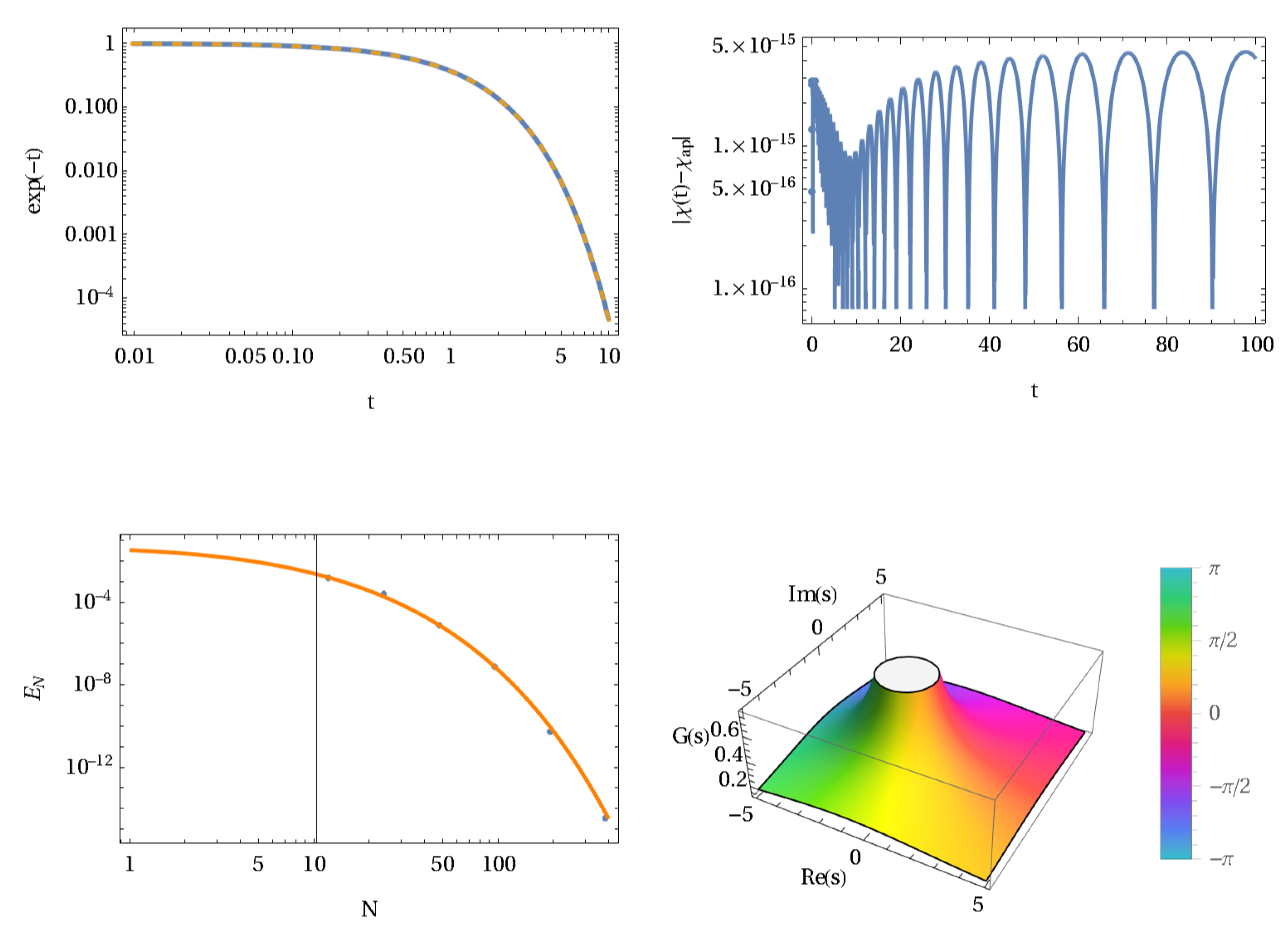
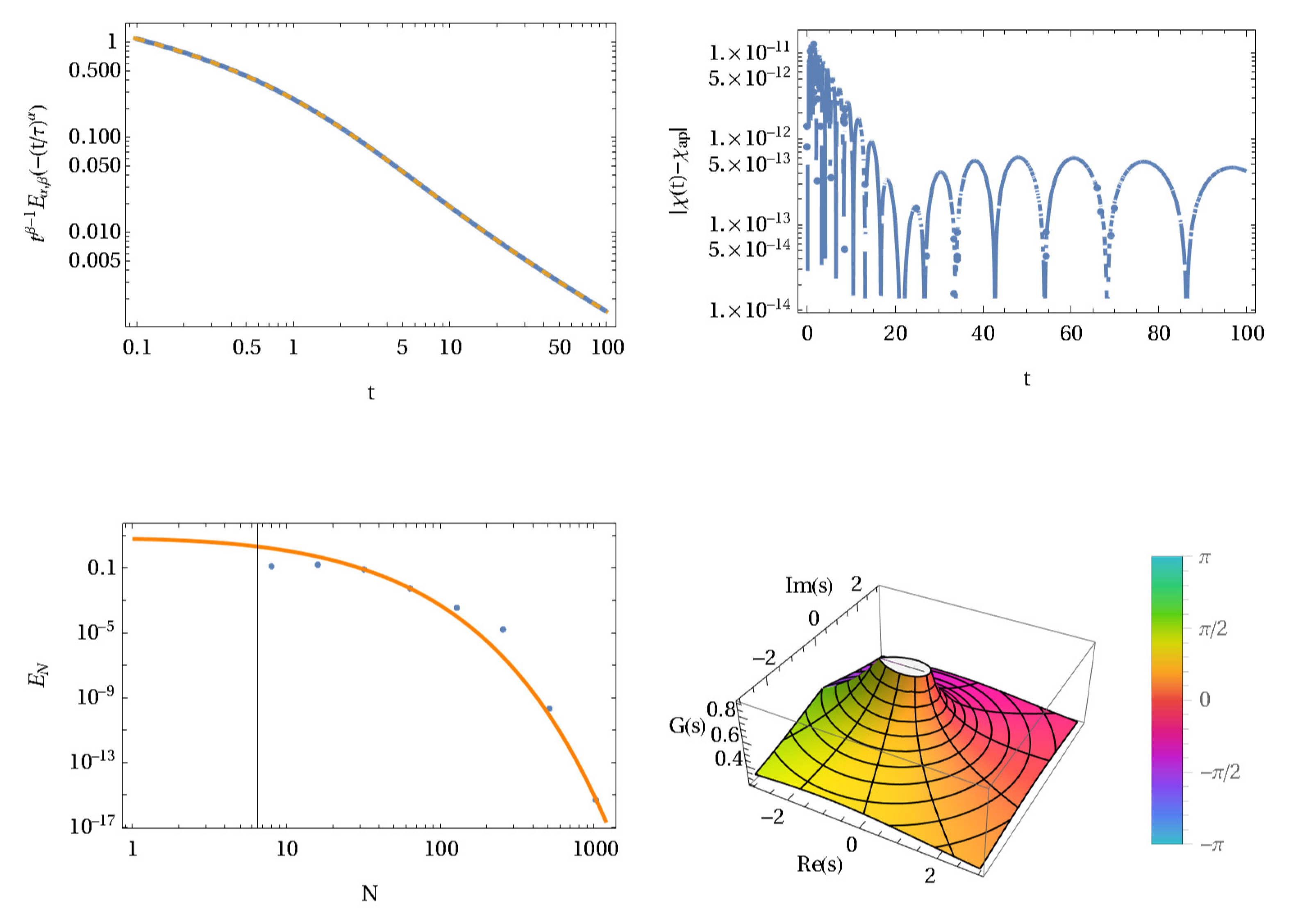
The relations were examined numerically by computing the eigenvalues of the Hermitian matrix H = A m * A m with A m * the conjugate transpose of A m . The results for different size ν = m × m matrices are shown in Figure 1. The left panel in Figure 1 is related to the pure Sinc basis, while the right panel represents results for the Sinc-Gaussian basis. It is obvious that, for the Sinc-Gaussian, the limits are symmetric to λ = 1 . In all cases, the relation between λ and the size ν of H follows a power law λ ν γ . The value for γ for the upper limit λ M is estimated to be nearly ν = 1 / 2 . For the lower limit λ m , the exponents are different. In the Sinc-Gaussian case, we find ν 1 / 2 , while the pure Sinc case shows a much smaller value of ν 7 / 100 . However, in both cases, the lower limit is a positive decaying function that is always greater than zero. Only in the limit ν is the value zero reached. This, in turn, tells us, based on Grenander and Szegö theory [42], that the eigenvalues of A m are strictly positive for finite matrix sizes.

2.3. Convolution Integrals

Indefinite convolution integrals can also be effectively collocated via Sinc methods [38]. This section discusses the core procedure of this paper, for collocating the convolution integrals and for obtaining explicit approximations of the functions p and q defined by
p ( x ) = a x f ( x t ) g ( t ) d t with x ( a , b ) ,
q ( x ) = x b f ( t x ) g ( t ) d t with x ( a , b ) ,
where x Γ . In presenting these convolution results, we shall assume that Γ = ( a , b ) R , unless otherwise indicated. Note also that being able to collocate p and q enables us to collocate definite convolutions, like a b f ( x t ) g ( t ) d t .
Before we start to present the collocation of the Equations (68) and (69), we mention that there is a special approach to evaluate the convolution integrals by using a Laplace transform. Lubich [43] introduced this way of calculation by the following idea
p ( x ) = 0 x f ( x t ) g ( t ) d t = 1 2 π i C F + ( s ) 0 x e s t g ( x t ) d t d s ,
for which the inner integral solves the initial value problem y = s y + g with g ( 0 ) = 0 . We assume that the Laplace transform
F + ( s ) = E f ( t ) e t / s d t ,
with E any subset of R such that E ( 0 , b a ) , exists for all s Ω + = { s C | ( s ) > 0 } .
In the notation introduced above, we get that
p = F + J + g F + J m + g
and
q = F + J g F + J m g
are accurate approximations, at least for g in a certain space [32]. The procedure to calculate the convolution integrals is now as follows. The collocated integral J m + = V m ( B ) · A m V m and J m = V m ( B ) · B m V m , upon diagonalization of A m and B m in the form
A m = X m · diag s m , M , , s m , N · X m 1 ,
B m = Y m · diag s m , M , , s m , N · Y m 1 ,
with Σ = diag s M , , s N as the eigenvalues arranged in a diagonal matrix for each of the matrices A m and B m . Then, the Laplace transform (71), introduced by Stenger, delivers the square matrices F + A m and F + B m defined via the equations
F + A m = X m · diag F + s m , M , , F + s m , N · X m 1 = X m F + ( Σ ) · X m 1 ,
F + B m = Y m · diag F + s m , M , , F + s m , N · Y m 1 = Y m F + ( Σ ) · Y m 1 .
We can get the approximation of (72) and (73) by
F + J + g F + J m + g = V m ( B ) · F + A m · V m ( g )
= V m ( B ) · X m F + ( Σ ) · X m 1 · V m ( g ) , F + J g F + J m g = V m ( B ) · F + B m · V m ( g )
= V m ( B ) · Y m F + ( Σ ) · Y m 1 · V m ( g ) .
These two formulas deliver a finite approximation of the convolution integrals p and q. The convergence of the method is exponential as was proved in Reference [38].

2.4. Inverse Laplace Transform

The inversion formula for Laplace transform inversion was originally discovered by Stenger in Reference [32]. This exact formula presented here is only the third known exact formula for inverting the Laplace transform, the other two being due to Post [44] and Bromwich [21], although we believe that practical implementation of the Post formula has never been achieved, while the evaluation of the vertical line formula of Bromwich is both far more difficult and less accurate than our method, which follows.
Let the Laplace transform F + be defined as in (71). If J + denotes the indefinite integral operator defined on ( 0 , a ) ( 0 , c ) ( 0 , ) , then the exact inversion formula is
f = J + 1 F + J + 1 ,
where 1 denotes the function that is identically 1 on ( 0 , a ) . Hence, with J m + w A m V , with A m = X S X 1 , S = diag s M , , s N , we can proceed as follows to compute the values f j f x j of f:
Assume that matrix X and vector s = s M , , s n T have already been computed from A m ; then, compute the column vector v = v M , , v N T = X 1 1 , where 1 is a vector of M + N + 1 ones:
Compute
g F + s M / s M , , F + s N / s N ,
z g v with a Hadamard product ,
f f M , , f N = X z .
All operations of this evaluation take a trivial amount of time, except for the last matrix-vector evaluation. However, the size of these matrices is nearly always much smaller than the size of the DFT matrices for solving similar problems via FFT.
Then, we have the approximation f x j f j , which we can combine, if necessary, with our interpolation Formula (33) to get a continuous approximation of f on ( 0 , a ) .

3. Numerical Examples

The following examples demonstrate the theoretical steps discussed above. To simplify the presentation we shall consider the symmetric approximation with M = N in the following. Thus, the step length is simplified to h = σ π / N and σ R + (see Reference [30] for details). We select starting from the very simple Debye model, the one-parameter fractional relaxation equation, its extension to two-parameter fractional relaxation equation to the three-parameter Prabhakar relaxation. Each of these models is related to an ML function with one, two, and three parameters. We will not extend this to higher-order ML functions because this is a straightforward process (see, e.g., Kilbas et al. [15]). As already introduced, we will use for our computations the transfer function G ( s ) as the basis for our approach to gain the time-dependent approximation or the representation of the ML function. Besides, we shall extend the ML functions to variable order functions useful to solve fractional differential or integral equations using variable orders.

3.1. Debye Model

To demonstrate the procedure, let us examine the classical Debye relaxation equation as initial value problem
d χ ( t ) dt = τ 1 χ ( t ) , with χ ( 0 ) = χ 0 .
The Laplace transform of the above equation delivers the algebraic equation
s L χ ( t ) = χ 0 τ 1 L χ ( t ) .
The solution of this equation in Laplace space follows by solving the above equation for the Laplace representation of χ :
L χ ( t ) = χ 0 s + τ 1 = G ( s ) .
Inverting this transfer function G ( s ) using inverse Laplace transforms the exact solution follows
χ ( t ) = χ 0 exp ( ( t / τ ) ) = χ 0 E 1 ( ( t / τ ) ) .
The first approach to get the solution χ ( t ) is to use a Sinc approximation of the transfer function G ( s ) . We use here the representation of G ( s ) on R + , i.e., we use a conformal map ψ generating the discrete Sinc points on ( 0 , ) . Note, we do not approximate the upper limit by a finite number. The result is an approximation of the transfer function G ( s ) G ˜ ( s ) = p μ ( s ) / q ν ( s ) , where p μ and q ν are polynomials of order μ and ν satisfying μ ν , which is a prerequisite of Heaviside’s theorem. The discrete set of data s k , G s k k = N N is then used in a continued fraction approximation of Thiele’s algorithm (for details, see References [2,30]). This approximation allows us to convert the rational expression using fractional exponents to a rational expression using integer exponents. The result of this approximation is shown in Figure 2. The left panel shows the original irrational fractional transfer function G ( s ) and its approximation using Thiele’s algorithm. It is obvious that, between the original function and its approximation, there is no visible difference. However, the local error between the exact and approximated function is shown in the right panel of Figure 2. First, we observe in Figure 2 that the error is a small quantity and that, for larger values of s, the local error decays more than 4 decades.
If the approximation of the transfer function is known as a symbolic rational expression, it becomes straightforward using Heaviside’s expansion theorem for inverse Laplace transforms to find the symbolic solution for the fractional relaxation equation. Heaviside’s theorem tells us that the fractional approximation can be represented in terms of exponential functions. The application of the inverse Laplace transform to the approximation of the transfer function G ˜ ( s ) delivers the graphs shown in Figure 3.
To demonstrate the application of the inverse Laplace transform based on indefinite integrals to Debye’s model, we apply the computations to the Equation (86) using the approach of Section 2.4. For this reason, we select a fixed set of parameters and vary the number of Sinc points to generate different approximations of order 2 N + 1 . This allows us to check the convergence of the algorithm stated in Equation (57) with c = 0 . The resulting errors computed using an L 2 norm estimation enables us to verify the error formula by determining two parameters the amplitude K 1 and the scaling parameter in the exponent k 1 . The results of the inversion of G ( s ) is shown in Figure 4 in connection with the local error and the decay of the error E N . In addition, we also depicted the transfer function G ( s ) on the complex plane to identify the location of the pole.

3.2. One Parameter Fractional Relaxation Equation

The canonical fractionalization of Debye’s initial value problem delivers a simple fractional relaxation equation
D α χ ( t ) = τ α χ ( t ) + χ 0 t α Γ ( 1 α ) ,
where D α represents the Riemann-Liouville operator, and α the fractional order is limited to 0 < α 1 [25]. χ 0 is the initial condition, and τ the fractional relaxation time. The Laplace transform of Equation (88) delivers the algebraic equation
s α L χ ( t ) = χ 0 s α 1 τ α L χ ( t ) .
The solution of this equation in Laplace space follows by solving the above equation for the Laplace representation of χ :
L χ ( t ) = χ 0 s α 1 s α + τ α = G ( s ) .
Inverting this transfer function using inverse Laplace transforms and Mellin transforms [25] will deliver the exact solution
χ ( t ) = χ 0 E α ( t / τ ) α .
To approximate Equation (90), we again use the Sinc-Thiele approximation of the fractional rational transfer function G ( s ) by using Thiele’s algorithm of continued fractions allowing us to convert the fractional rational function G ( s ) to an integer exponent rational G ˜ ( s ) shown in Figure 5. The figure demonstrates that an efficient approximation within a small error is possible, thus allowing the application of Hamilton’s method.
The use of a partial fraction expansion and a direct inversion of the resulting fraction representation again delivers a finite series of exponential functions representing the solution of the fractional differential Equation (88) (see Figure 6).
Applying the second method of Laplace inversion based on pure Sinc approximations ( c = 0 ) to the fractional transfer function delivers the inverse Laplace transforms for the selected parameters. Some results are shown in Figure 7. The results in this figure are the approximation of the one-parameter ML function E α ( t / τ ) α for α = 3 / 4 . Compared with the results in Figure 6, we observe that, for a sufficiently large number of Sinc points, we can reach a relatively small absolute error in our approximation (see the top right panel in Figure 7). To compute this absolute local error, we used the implemented ML function in Mathematica as reference, knowing that this representation is also based on approximations. In addition, it is also clear that we have exponential convergence of the method following the estimates of Equation (57) shown as a two-parameter least-square fit to the computed L 2 norm E N (bottom left panel in Figure 7). The bottom right panel shows the location of the pole of the transfer function G ( s ) in the complex plane. The colors on the surface represent the argument varying from π to π . The branch cut of the transfer function is on the negative real axis.
In Figure 8, we depict a collection of ML functions E α ( t / τ ) α for varying values of α . The graph includes the approximation using an inverse Laplace transform based on pure Sinc approximations (solid line) and the Mathematica representation (dashed line). It is apparent that the Sinc approximation and the Mathematica implementation of the ML function agree on a larger scale. The character of the one parameter ML function E α does not change dramatically only the decay to zero is a characteristic included in this graph.

3.3. Two Parameter Fractional Relaxation Equation

The approximation of the two-parameter ML function is demonstrated by a two-parameter relaxation model. We use for this model the SG approximation of the inverse Laplace transform. The reason for using SG instead of Sinc is that the eigenvalues of the SG approximation are clustered closer to zero in the complex plane, while the Sinc distribution of eigenvalues is slightly moved away from zero. This is controlled by the value c = 1 / 150 , which is the same in all SG computations.
To demonstrate the SG method, let us consider a simple fractional relaxation equation which may be used to define the two-parameter Mittag-Leffler function as a solution. The equation represents a two-parameter fractional relaxation process given by
D α χ ( t ) = τ α χ ( t ) + χ 0 t β α 1 Γ ( β α ) ,
where α and β are positive numbers which we restrict to 0 < α , β 1 , and χ 0 is the initial condition. The Laplace transform of the above equation delivers the algebraic equation
s α L χ ( t ) = χ 0 s α β τ α L χ ( t ) .
The solution of this equation in Laplace space follows by solving Equation (93) for the Laplace representation of χ :
L χ ( t ) = χ 0 s α β s α + τ α = G ( s ) .
Note that, for α < β , the transfer function changes its character in the complex plane. From a pole-dominated characteristic, it changes to a singularity-dominated function if α < β . This change causes some problems in the approximation which become obvious if β < 1 . The assumption in the fractional model that β < 1 is not restrictive in mathematical terms and can be relaxed to values β > 1 . However, from a physical point of view, as a relaxation model, β should be less than 1. In the following, we will consider both cases. The important point here is that, for α < β , the structure of the ML function in Laplace space will change.
Inverting analytically the two-parameter transfer function using the inverse Laplace transforms and Mellin transforms [25] will deliver the exact solution which can be represented by a two-parameter Mittag-Leffler function
χ ( t ) = χ 0 t β 1 E α , β ( t / τ ) α .
To demonstrate the approximation of the solution, let us first apply the Sinc-Thiele approach. To approximate Equation (94), we use a Sinc approximation of the fractional rational transfer function G ( s ) by Thiele’s algorithm of continued fractions allowing us to convert the fractional rational function G ( s ) to an integer exponent rational G ˜ ( s ) shown in Figure 9. The figure demonstrates that an effective approximation within a small error is possible, thus allowing the application of Hamilton’s method.
The use of a partial fraction expansion and a direct inversion of the resulting fraction representation again delivers a finite series of exponential functions representing the solution of the fractional differential Equation (92), as shown in Figure 10.
It is obvious from the results shown in Figure 10 that an approximation of the solution of a fractional initial value problem is a direct method and delivers an accurate result with a minimal amount of computation steps. The steps needed are reduced to the collocation of the transfer function, which is approximated by Thiele’s algorithm as a continued fraction. This continued fraction is converted to a rational expression which is used in a Laplace inversion to get the solution. Such kind of inversion is always possible if the conditions for Heaviside’s expansion theorem are satisfied. Thus, any rational fraction of polynomials can be represented by a finite sum of exponentials if the inverse Laplace transform is applied to this rational fraction in Laplace space.
Applying the third method of Laplace inversion based on SG approximations to the fractional transfer function delivers the inverse Laplace transform for the selected parameters. Some results are shown in Figure 11. The results in Figure 11 are the approximation of the two-parameter ML function t β 1 E α , β ( t / τ ) α for α = 2 / 3 and β = 3 / 4 . Compared with the error in Figure 10, we observe that, for a sufficiently large number of Sinc points, we can reach a relatively small absolute error in our approximation (see the top right panel in Figure 11). To compute this absolute local error, we used the implemented ML function in Mathematica as reference. Besides, it is also clear that we have exponential convergence of the method following the estimates of Equation (57) shown as a two-parameter least-square fit to the computed L 2 norm E N (bottom left panel in Figure 11). The bottom right panel shows the location of the pole of the transfer function G ( s ) in the complex plane. The colors on the surface represent the argument varying from π to π . The branch cut of the transfer function is on the negative real axis.
To demonstrate the variety of the ML function by changing the first parameter α and keeping the second fixed at β = 11 / 9 , we graph in Figure 12 a family of curves. The variation from an increasing function to a decreasing and oscillating function shows the different behaviors of E α , β .
Figure 13 demonstrates that the SG inverse Laplace transform still works under fairly regular conditions if β is not far below α . This is the case where the transfer function G ( s ) is dominated by a singularity at zero. The accuracy of the approximation is still valid with an L 2 error of approximately 10 3 .

3.4. Three Parameter Fractional Relaxation Equation: Prabhakar Function

A special type of ML function is the Prabhakar function. It was introduced by T.R. Prabhakar in 1971 in connection with weakly singular Volterra integral equations [18]. A subset of these functions is currently used in literature to describe anomalous dielectric relaxation [45,46]. These Havriliak-Negami models are also used to describe the dielectric and viscous properties of polymeric material [47]. However, Prabhakar’s generalization of ML functions to three parameters is not the only ML function using three parameters; for a general discussion, see Reference [15]. Due to the application to polymeric material and the connection to fractional calculus, we shall restrict our discussions to Prabhakar’s transfer function
χ ^ ( s ) = χ 0 s γ α β s α + τ α γ = G ( s ) .
The first approach to approximate Prabhakar’s function using (96) is our Sinc-Thiele approximation using a finite number of Sinc points to approximate the transfer function G ( s ) . The result is shown in Figure 14.
The result is an approximation of the transfer function G ( s ) G ˜ ( s ) = p μ ( s ) / q ν ( s ) , where p μ and q ν are polynomials of order μ and ν satisfying μ ν , which is a prerequisite of Heaviside’s theorem. The approximated fraction G ˜ ( s ) and the original expression for the transfer function G ( s ) is shown in Figure 14. The left panel shows the original irrational fractional transfer function G ( s ) and its approximation using Thiele’s algorithm. It is obvious that, between the original function and its approximation, there is no visible difference. However, the local error between the exact and approximated function is shown in the right panel of Figure 14.
If the approximation of the transfer function is known as a symbolic rational expression, it becomes straightforward using Heaviside’s expansion theorem for inverse Laplace transforms to find the symbolic solution for the fractional relaxation equation (see Figure 15). We also included the two-parameter ML function (dashed line) in this figure to demonstrate the deviations of Prabhakar’s function from the two-parameter ML function shown in the right panel.
Applying the third method of Laplace inversion based on SG approximations to the fractional transfer function of Prabhakar’s function delivers the inverse Laplace transform for the selected parameters. Some results are shown in Figure 16. Figure 16 shows the approximation of the three-parameter ML function t β 1 E α , β γ ( t / τ ) α for α = 7 / 10 . The three panels on the left demonstrate the changes of the Prabhakar function if β and γ are varied. The right graphs are representing the relative local error. As a reference we computed the truncated series (3) with 126 terms, which is called χ ( t ) in the graphs. It is apparent that, for all three-parameter choices, we achieved a relatively small local error. It is also remarkable that a relatively small change in the parameter values results in completely different function behavior (see Figure 16).
In Figure 17, we collect a variety of solutions for the HN model, where β = α γ . We compare the series representation of Prabhakar’s function by the SG inverse Laplace solution for different parameters γ . Note the range of the graphs is restricted to a few decades due to the inaccurate numerical results of the series approximation for large arguments. The SG inverse Laplace transform is, however, capable of covering much more decades than are shown in Figure 17.
Figure 18 demonstrates that the SG inverse Laplace transforms still works under general choices of parameters. The graphs are related to a model, where β = 2 α γ with fixed α and varying γ . The right panel demonstrates that the SG inverse Laplace transform can cover three decades and more by using a relatively small number of Sinc points.

3.5. Scarpi’s Variable-Order Fractional Calculus

The SG inverse Laplace transform even works for variable-order calculus. We follow Scarpi’s approach for a relaxation problem [48]. In a recent paper, Garrappa et al. [49] discussed a variable order fractional calculus in connection with fractional relaxation equations. Scarpi’s fractional initial value problem is stated as follows:
D α ( t ) χ ( t ) = τ χ ( t ) , and χ ( 0 ) = χ 0 .
The transfer function of this problem is given after a Laplace transform and some algebraic manipulations as
G ( s ) = s s α ^ ( s ) 1 χ 0 s s α ^ ( s ) + τ ,
where α ^ ( s ) is the Laplace transform of α ( t ) . For details of the theoretical back ground, see Reference [49]. Figure 19 shows the solution χ ( t ) for different models of α ( t ) = 1 t k e t with k = 0 , 1 , 2 , 3 . The case with k = 0 reproduces one example in Reference [49], while the other cases are solutions satisfying the conditions given in Reference [49].
Following the ideas of Scarpi, Wiman, and Prabhakar, we are also able to generalize the variable order transfer function to the cases of two and three variable exponents in the transfer function G ( s ) . For the Wiman extension, we can write
G ( s ) = s s α ^ ( s ) s β ^ ( s ) χ 0 s s α ^ ( s ) + τ ,
and, for the Prabhakar extension, we get
G ( s ) = s s 2 α ^ ( s ) γ ^ ( s ) s β ^ ( s ) χ 0 s s α ^ ( s ) + τ s γ ^ ( s ) .
Both transfer functions can be used in the SG inverse Laplace transform to generate the solutions for given functions α ( t ) , β ( t ) , and γ ( t ) (see Figure 20).
We note that these generalizations of the transfer functions are related to a fractional differential or integral equations using variable exponents α , β , and γ .

4. Conclusions

The paper discusses exact versions of the inverse Laplace transform in connection with Mittag-Leffler functions involving three parameters. The Sinc-Gaussian inverse Laplace transform is an exact inversion of the Laplace transform and uses Sinc-Gaussian basis functions for approximation. It turns out that the eigenvalues of the matrix A m are the essential properties of the approximation which all satisfy λ k > 0 . However, the SG basis shows some advantages over the pure Sinc version because the SG eigenvalues are moved in the direction of the origin in such a way that stability and convergence compared with the pure Sinc representation is improved. This property allows us to use relatively small matrices to represent the inverse Laplace transform on R + . Moreover, the method is free of any Bromwich contour and converges exponentially. In addition, the Sinc or SG inverse Laplace transform needs a minimal amount of coding, thus being very useful in practical applications. It turned out that the method can be effectively used to represent Mittag-Leffler functions of one, two, and three parameters. Even for variable-order fractional differential or integral equations, the SG inverse Laplace method is a powerful tool.
The three methods presented can be used either as a reference in computing or as a straightforward computing tool in systems design and fractional calculus to gain effective numerical approximations.

Funding

This research received no external funding.

Institutional Review Board Statement

Not applicable.

Informed Consent Statement

Not applicable.

Data Availability Statement

Not applicable.

Acknowledgments

I acknowledge the inspiring discussions and valuable ideas by Frank Stenger.

Conflicts of Interest

There is no conflict of interest.

References

  1. Stenger, F.; Baumann, G.; Koures, V.G. Computational Methods for Chemistry and Physics, and Schrödinger in 3 + 11. In Advances in Quantum Chemistry; Elsevier: Amsterdam, The Netherlands, 2015; Volume 71, pp. 265–298. ISBN 978-0-12-802824-7. [Google Scholar]
  2. Baumann, G.; Stenger, F. Sinc-Approximations of Fractional Operators: A Computing Approach. Mathematics 2015, 3, 444–480. [Google Scholar] [CrossRef] [Green Version]
  3. Baumann, G.; Stenger, F. Fractional Calculus and Sinc Methods. Fract. Calc. Appl. Anal. 2011, 14, 568–622. [Google Scholar] [CrossRef]
  4. Schmeisser, G.; Stenger, F. Sinc Approximation with a Gaussian Multiplier. Sampl. Theory Signal Image Process. 2007, 6, 199–221. [Google Scholar] [CrossRef]
  5. Talbot, A. The Accurate Numerical Inversion of Laplace Transforms. IMA J. Appl. Math. 1979, 23, 97–120. [Google Scholar] [CrossRef]
  6. López-Fernández, M.; Palencia, C. On the Numerical Inversion of the Laplace Transform of Certain Holomorphic Mappings. Appl. Numer. Math. 2004, 51, 289–303. [Google Scholar] [CrossRef]
  7. López-Fernández, M.; Palencia, C.; Schädle, A. A Spectral Order Method for Inverting Sectorial Laplace Transforms. SIAM J. Numer. Anal. 2006, 44, 1332–1350. [Google Scholar] [CrossRef] [Green Version]
  8. Weideman, J.A.C.; Trefethen, L.N. Parabolic and Hyperbolic Contours for Computing the Bromwich Integral. Math. Comp. 2007, 76, 1341–1357. [Google Scholar] [CrossRef] [Green Version]
  9. Garrappa, R. Numerical Evaluation of Two and Three Parameter Mittag-Leffler Functions. SIAM J. Numer. Anal. 2015, 53, 1350–1369. [Google Scholar] [CrossRef] [Green Version]
  10. Baumann, G. Mathematica for Theoretical Physics, 2nd ed.; Springer: New York, NY, USA, 2005; ISBN 978-0-387-01674-0. [Google Scholar]
  11. Glöckle, W.G.; Nonnenmacher, T.F. A Fractional Calculus Approach to Self-Similar Protein Dynamics. Biophys. J. 1995, 68, 46–53. [Google Scholar] [CrossRef] [Green Version]
  12. Baumann, G.; Südland, N.; Nonnenmacher, T.F. Anomalous Relaxation and Diffusion Processes in Complex Systems. Transp. Theory Stat. Phys. 2000, 29, 157–171. [Google Scholar] [CrossRef]
  13. Mainardi, F. Fractional Calculus and Waves in Linear Viscoelasticity: An Introduction to Mathematical Models; Imperial College Press: London, UK; Hackensack, NJ, USA, 2010; ISBN 978-1-84816-329-4. [Google Scholar]
  14. Gorenflo, R.; Kilbas, A.A.; Mainardi, F.; Rogosin, S.V. Mittag-Leffler Functions, Related Topics and Applications; Springer Monographs in Mathematics; Springer: Berlin/Heidelberg, Germany, 2014; ISBN 978-3-662-43929-6. [Google Scholar]
  15. Kilbas, A.A.; Srivastava, H.M.; Trujillo, J.J. Theory and Applications of Fractional Differential Equations. In North-Holland Mathematics Studies, 1st ed.; Elsevier: Amsterdam, The Netherlands; Boston, MA, USA, 2006; ISBN 978-0-444-51832-3. [Google Scholar]
  16. Mittag-Leffler, M.G. Sur l’intégrale de Laplace-Abel. C. R. Acad. Sci. Paris (Ser. II) 1902, 136, 937–939. [Google Scholar]
  17. Wiman, A. Über den Fundamentalsatz in der Teorie der Funktionen Eα(x). Acta Math. 1905, 29, 191–201. [Google Scholar] [CrossRef]
  18. Prabhakar, T.R. A Singular Integral Equation with a Generalized Mittag-Leffler Function in the Kernel. Yokohama Math. J. 1971, 19, 7–15. [Google Scholar]
  19. Garrappa, R.; Popolizio, M. Fast methods for the computation of the Mittag-Leffler function. In Handbook of Fractional Calculus with Applications; Kochubei, A.N., Luchko, Y.F., Karniadakis, G., Tarasov, V.E., Petráš, I., Baleanu, D., Lopes, A.M., Eds.; De Gruyter: Berlin, Germany; Boston, MA, USA, 2019; Volume 3, pp. 329–346. ISBN 978-3-11-057081-6. [Google Scholar]
  20. Giusti, A.; Colombaro, I.; Garra, R.; Garrappa, R.; Polito, F.; Popolizio, M.; Mainardi, F. A Practical Guide to Prabhakar Fractional Calculus. Fract. Calc. Appl. Anal. 2020, 23, 9–54. [Google Scholar] [CrossRef] [Green Version]
  21. Bromwich, T.J.I. Normal Coordinates in Dynamical Systems. Proc. Lond. Math. Soc. 1917, s2-15, 401–448. [Google Scholar] [CrossRef] [Green Version]
  22. Ang, D.D.; Lund, J.; Stenger, F. Complex Variable and Regularization Methods of Inversion of the Laplace Transform. Math. Comp. 1989, 53, 589–608. [Google Scholar] [CrossRef]
  23. Davies, B.; Martin, B. Numerical Inversion of the Laplace Transform: A Survey and Comparison of Methods. J. Comput. Phys. 1979, 33, 1–32. [Google Scholar] [CrossRef]
  24. Debye, P. Zur Theorie der spezifischen Wärmen. Ann. Phys. 1912, 344, 789–839. [Google Scholar] [CrossRef] [Green Version]
  25. Baumann, G. Mathematica for Theoretical Physics; Springer: New York, NY, USA, 2013; Volumes I and II. [Google Scholar]
  26. Südland, N.; Baumann, G.; Nonnenmacher, T.F. Fractional Driftless Fokker-Planck Equation with Power Law Diffusion Coefficients. In Computer Algebra in Scientific Computing CASC 2001, Proceedings of the Fourth International Workshop on Computer Algebra in Scientific Computing, Konstanz, Germany, 22–26 September 2001; Ganzha, V.G., Mayr, E.W., Vorozhtsov, E.V., Eds.; Springer: Berlin/Heidelberg, Germany, 2001; p. 513. ISBN 978-3-642-56666-0. [Google Scholar]
  27. Kilbas, A.A.; Saigo, M.; Saxena, R.K. Solution of Volterra Integro-Differential Equations with Generalized Mittag-Leffler Function in the Kernels. J. Integral Equ. Appl. 2002, 14, 377–396. [Google Scholar] [CrossRef]
  28. Podlubny, I. Fractional Differential Equations: An Introduction to Fractional Derivatives, Fractional Differential Equations, to Methods of Their Solution and Some of Their Applications. In Mathematics in Science and Engineering; Academic Press: San Diego, CA, USA, 1999; ISBN 978-0-12-558840-9. [Google Scholar]
  29. Roy, S.D. On the Realization of a Constant-Argument Immittance or Fractional Operator. IEEE Trans. Circ. Theory 1967, 14, 264–274. [Google Scholar] [CrossRef]
  30. Stenger, F. Numerical Methods Based on Sinc and Analytic Functions; Springer Series in Computational Mathematics; Springer: New York, NY, USA, 1993; Volume 20, ISBN 978-1-4612-7637-1. [Google Scholar]
  31. Stenger, F.; El-Sharkawy, H.A.; Baumann, G. The Lebesgue Constant for Sinc Approximations. In New Perspectives on Approximation and Sampling Theory: Festschrift in Honor of Paul Butzer’s 85th Birthday; Zayed, A.I., Schmeisser, G., Eds.; Applied and Numerical Harmonic Analysis; Springer International Publishing: Cham, Switzerland, 2014; ISBN 978-3-319-08800-6. [Google Scholar]
  32. Stenger, F. Handbook of Sinc Numerical Methods. In Chapman & Hall/CRC Numerical Analysis and Scientific Computing; CRC Press: Boca Raton, FL, USA, 2011; ISBN 978-1-4398-2158-9. [Google Scholar]
  33. Baumann, G. New Sinc Methods of Numerical Analysis: Festschrift in Honor of Frank Stenger’s 80th Birthday; Springer Nature: Cham, Switzerland, 2021; ISBN 978-3-030-49715-6. [Google Scholar]
  34. Qian, L.; Creamer, D.B. Localization of the Generalized Sampling Series and Its Numerical Application. SIAM J. Numer. Anal. 2006, 43, 2500–2516. [Google Scholar] [CrossRef]
  35. Qian, L. On the Regularized Whittaker-Kotel’nikov-Shannon Sampling Formula. Proc. Am. Math. Soc. 2003, 131, 1169–1176. [Google Scholar] [CrossRef]
  36. Butzer, P.L.; Stens, R.L. A Modification of the Whittaker-Kotelnikov-Shannon Sampling Series. Aeq. Math. 1985, 28, 305–311. [Google Scholar] [CrossRef]
  37. Shen, X.; Zayed, A.I. (Eds.) Multiscale Signal Analysis and Modeling; Springer: New York, NY, USA, 2013; ISBN 978-1-4614-4144-1. [Google Scholar]
  38. Stenger, F. Collocating Convolutions. Math. Comput. 1995, 64, 211–235. [Google Scholar] [CrossRef]
  39. Han, L.; Xu, J. Proof of Stenger’s Conjecture on Matrix I(-1) of Sinc Methods. J. Comput. Appl. Math. 2014, 255, 805–811. [Google Scholar] [CrossRef]
  40. Gray, R.M. Toeplitz and Circulant Matrices. A Review; Now: Boston, MA, USA, 2006. [Google Scholar]
  41. Trench, W.F. Spectral Evolution of a One-Parameter Extension of a Real Symmetric Toeplitz Matrix. SIAM J. Matrix Anal. Appl. 1990, 11, 601–611. [Google Scholar] [CrossRef]
  42. Grenander, U.; Szegö, G. Toeplitz Forms and Their Applications, 2nd (textually unaltered) ed.; Chelsea Pub. Co.: New York, NY, USA, 1984; ISBN 978-0-8284-0321-4. [Google Scholar]
  43. Lubich, C. Convolution Quadrature and Discretized Operational Calculus. II. Numer. Math. 1988, 52, 413–425. [Google Scholar] [CrossRef]
  44. Post, E. Generalized Differentiation. Trans. AMS 1930, 32, 723–781. [Google Scholar] [CrossRef]
  45. Khamzin, A.A.; Nikitin, A.S. Trap-Controlled Fractal Diffusion Model of an Atypical Dielectric Response. Chem. Phys. 2021, 111163. [Google Scholar] [CrossRef]
  46. Bia, P.; Caratelli, D.; Mescia, L.; Cicchetti, R.; Maione, G.; Prudenzano, F. A Novel FDTD Formulation Based on Fractional Derivatives for Dispersive Havriliak-Negami Media. Signal Process. 2015, 107, 312–318. [Google Scholar] [CrossRef]
  47. Garrappa, R. Grünwald-Letnikov Operators for Fractional Relaxation in Havriliak-Negami Models. Commun. Nonlinear Sci. Numer. Simul. 2016, 38, 178–191. [Google Scholar] [CrossRef]
  48. Scarpi, G. Sulla Possibilità Di Un Modello Reologico Intermediodi Tipo Evolutivo. Atti Accad. Naz. Lincei Rend. Cl. Sci. Fis. Mat. Nat. 1972, 52, 912–917. [Google Scholar]
  49. Garrappa, R.; Giusti, A.; Mainardi, F. Variable-Order Fractional Calculus: A Change of Perspective. arXiv 2021, arXiv:2102.09932. [Google Scholar]
Figure 1. Limits for eigenvalues of the Hermitian Matrix H = A m * A m . Left panel shows the minimal and maximal eigenvalues for a Sinc basis and the right panel for a Sinc-Gaussian basis (log-log plot). The limits follow a relation λ n , M ν ± γ with ν = m × m the size of H, and γ 1 / 2 for the upper limits and γ 7 / 100 for the lower limit of a Sinc approximation. The lower limit for Sinc-Gaussian follows the upper limit with the opposite sign.
Fractalfract 05 00043 g001
Figure 2. Approximation of the transfer function G ( s ) for the Debye relaxation equation given by (84). The left panel shows the exact transfer function G ( s ) with χ 0 = 1 and τ = 1 in connection with the approximation G ˜ ( s ) using Thiele’s algorithm (dashed line). The right panel shows the local error between the exact transfer function and its approximation. The total number of points used in the approximation is m = 2 N + 1 = 35 .
Fractalfract 05 00043 g002
Figure 3. Solution of the Debye relaxation Equation (84) generated by the inverse Laplace transform of G ˜ ( s ) . The left panel also includes the exact solution of the relaxation equation given by χ ( t ) = χ 0 exp ( ( t / τ ) ) (dashed) and the approximation (solid line). The right panel shows the local error of the exact solution and the approximation. The number of approximation points used in the calculation was m = 2 N + 1 = 35 . The parameters to generate the plot are χ 0 = 1 and τ = 1 .
Fractalfract 05 00043 g003
Figure 4. Solution of Debye’s relaxation Equation (84) generated by the Sinc inverse Laplace transform based on indefinite integrals. The top left panel includes the exact solution of the relaxation equation given by χ ( t ) = χ 0 exp ( ( t / τ ) ) (dashed) and the approximation (solid line). The top right panel shows the absolute local error of the difference between the exact solution and the approximation. The number of approximation points used in the calculation was m = 2 N + 1 = 769 . The parameters to generate the plot are χ 0 = 1 and τ = 1 . The bottom panels (left) show the error decay as a function of Sinc points N, E N N exp k 1 N 1 / 2 . Dots represents numerically determined L 2 norms, and the solid line represents Equation (57) with c = 0 , where K 1 and k 1 are adapted accordingly. The right panel shows the structure of the transfer function G ( s ) on the complex plane C .
Fractalfract 05 00043 g004
Figure 5. Approximation of the transfer function G ( s ) for a fractional relaxation Equation (88). The left panel shows the exact transfer function G ( s ) with χ 0 = 1 , τ = 1 , and α = 2 / 3 in connection with the approximation G ˜ ( s ) using Thiele’s algorithm. The right panel shows the local error between the exact function G ( s ) and its approximation. The total number of points used in the approximation is m = 2 N + 1 = 35 .
Fractalfract 05 00043 g005
Figure 6. Solution of the fractional relaxation Equation (88) generated by the inverse Laplace transform of G ˜ ( s ) . The left panel also includes the exact solution of the fractional relaxation equation given by χ ( t ) = χ 0 E α ( t / τ ) α where E α ( t ) is the Mittag-Leffler function. The right panel shows the local error between the exact solution and the approximation. The number of approximation points used in the calculation was m = 2 N + 1 = 35 . The parameters to generate the plot are χ 0 = 1 , τ = 1 , α = 2 / 3 .
Fractalfract 05 00043 g006
Figure 7. Solution of the fractional relaxation Equation (90) generated by the inverse Laplace transform of G ( s ) . The left panel on top also includes the exact solution of the fractional relaxation equation given by χ ( t ) = χ 0 E α ( t / τ ) α , where E α ( t ) is the one parameter Mittag-Leffler function. The right panel on top shows the local error between the exact solution and the approximation. The number of approximation points used in the calculation was m = 2 N + 1 = 1025 . The parameters to generate the plot are χ 0 = 1 , τ = 1 , α = 3 / 4 . The bottom panels (left) show the error decay as a function of Sinc points N, E N N exp k 1 N 1 / 2 . Dots represent numerically determined L 2 norms, and the solid line represents Equation (57) with c = 0 , where K 1 and k 1 are adapted accordingly. The right panel shows the pole structure with a branch cut along the negative real axis of the transfer function G ( s ) on the complex plane C .
Fractalfract 05 00043 g007
Figure 8. A variety of solutions of (88) for different values of α . From top to bottom on the right end of the graph, the α values vary between 0.05 and 1 in steps of 0.01. The solid line represents the Sinc inverse Laplace result, while the dashed line is the Mathematica implementation of E α ( t / τ ) α . Parameters are χ 0 = 1 , τ = 1 , and N = 256 .
Fractalfract 05 00043 g008
Figure 9. Approximation of the transfer function G ( s ) for a fractional relaxation equation given by (94). The left panel shows the exact transfer function G ( s ) with χ 0 = 1 , τ = 1 , α = 1 / 2 , and β = 1 / 3 in connection with the approximation using Thiele’s algorithm. The right panel shows the local error between the exact function and its approximation. The total number of points used in the approximation is m = 2 N + 1 = 35 .
Fractalfract 05 00043 g009
Figure 10. Solution of the fractional relaxation Equation (92) generated by the inverse Laplace transform of G ˜ ( s ) . The left panel also includes the exact solution of the fractional relaxation equation given by χ ( t ) = χ 0 t β 1 E α , β ( t / τ ) α , where E α , β ( z ) is the two parameter Mittag-Leffler function. The right panel shows the local error between the exact solution and the approximation. The number of approximation points used in the calculation was m = 2 N + 1 = 35 . The parameters to generate the plot are χ 0 = 1 , τ = 1 , α = 1 / 2 , and β = 1 / 3 .
Fractalfract 05 00043 g010
Figure 11. Approximation of the fractional relaxation Equation (92) generated by the SG inverse Laplace transform of G ( s ) . The left panel on top includes the exact solution of the fractional relaxation equation given by χ ( t ) = χ 0 t β 1 E α , β ( t / τ ) q , where E α , β ( t ) is the Mittag-Leffler function. The right panel on top shows the local error between the exact solution and the approximation. The number of approximation points used in the calculation was m = 2 N + 1 = 2049 . The parameters to generate the plot are χ 0 = 1 , τ = 1 , α = 2 / 3 , and β = 3 / 4 . The bottom panels (left) show the error decay as a function of Sinc points N, E N N exp k 1 N 1 / 2 . Dots represents numerically determined L 2 norms, and the solid line represents Equation (57) with c = 1 / 150 , where K 1 and k 1 are adapted accordingly. The right panel shows the pole structure with a branch cut along the negative real axis of the transfer function G ( s ) on the complex plane C .
Fractalfract 05 00043 g011
Figure 12. A variety of solutions of (94) for different values of α . From top to bottom on the right end of the graph the α values vary between 0.1 and 1.5 in steps of 0.1 with β = 11 / 9 . The solid line represents the SG inverse Laplace result, while the overlaid dashed line is the Mathematica implementation of t β 1 E α , β ( t / τ ) α . Parameters are χ 0 = 1 , τ = 1 , and N = 96 .
Fractalfract 05 00043 g012
Figure 13. An example where the condition α < β is violated. Parameters are χ 0 = 1 , τ = 1 , α = 1 / 2 , and β = 7 / 20 . The pole of the transfer function is replaced by a singularity at zero (right panel).
Fractalfract 05 00043 g013
Figure 14. Approximation of the transfer function G ( s ) for a three parameter fractional relaxation equation represented by (96). The left panel shows the exact transfer function G ( s ) with χ 0 = 1 , τ = 1 , α = 1 / 2 , β = 2 / 3 , and γ = 9 / 10 in connection with the approximation using Thiele’s algorithm. The right panel shows the local error between the exact function and its approximation. The total number of point used in the approximation is m = 2 N + 1 = 35 .
Fractalfract 05 00043 g014
Figure 15. Solution of the fractional relaxation Equation (96) generated by the inverse Laplace transform of G ˜ ( s ) . The left panel also includes the two parameter ML function t β 1 E α . β ( t / τ ) α as a reference. The right panel shows the local error between the reference and the approximation. The number of approximation points used in the calculation was m = 2 n + 1 = 35 . The parameters to generate the plot are χ 0 = 1 , τ = 1 , α = 1 / 2 , β = 2 / 3 , and γ = 9 / 10 .
Fractalfract 05 00043 g015
Figure 16. Three different parameter selections for Prabhakar’s function χ ( t ) = χ 0 t β 1 E α , β γ ( t / τ ) q . The left panels include the SG approximation (solid line) and the series representation truncated by 126 terms. The right panels show the relative absolute local errors using the series approximation as reference. The number of approximation points used in the calculation was N = 128 . The parameter sets used from top to bottom are { χ 0 = 1 , τ = 1 , α = 7 / 10 , β = 3 / 10 , γ = 22 / 10 }, { χ 0 = 1 , τ = 1 , α = 7 / 10 , β = 3 / 10 , γ = 12 / 10 }, { χ 0 = 1 , τ = 1 , α = 7 / 10 , β = 9 / 10 , and γ = 8 / 10 }.
Fractalfract 05 00043 g016
Figure 17. A variety of solutions of the HN model with β = α γ for different values of γ . From top to bottom on the right end of the graph, the γ values varied and α kept fixed. The solid line represents the SG inverse Laplace result, while the dashed line is the series implementation of t β 1 E α , β γ ( t / τ ) α using 126 terms. The SG inverse Laplace results are not limited to the shown scale. The limitation results here by using the series representation. Parameters are χ 0 = 1 , τ = 1 , α = 1 / 2 , and γ is taken from [3/5,2] in steps of 1/10. The number of Sinc points is N = 128 .
Fractalfract 05 00043 g017
Figure 18. A variety of solutions with β = 2 α γ for different values of γ . The solid line represents the SG inverse Laplace result, while the dashed lines are the series approximation of t β 1 E α , β γ ( t / τ ) α using 126 terms. The limitation on the left panel for the range results from using the series representation and the bad convergence for large arguments. The right panel shows the same SG inverse Laplace transform on a wider range. Parameters are χ 0 = 1 , τ = 1 , α = 4 / 5 , and γ is taken from [2/5,2] in steps of 1/10. The number of Sinc points is N = 128 .
Fractalfract 05 00043 g018
Figure 19. Variable order fractional relaxation with α ( t ) = 1 t k e t and k = 0 , 1 , 2 , 3 . The number of Sinc points is N = 128 .
Fractalfract 05 00043 g019
Figure 20. Extensions of Scarpi’s fractional equation. Left panel α ( t ) = 1 cosh ( t ) 2 and β ( t ) = cosh ( t ) with N = 128 . Right panel the same functions for α ( t ) and β ( t ) as in the left panel, but γ ( t ) = sin ( t ) and N = 256 .
Fractalfract 05 00043 g020
Publisher’s Note: MDPI stays neutral with regard to jurisdictional claims in published maps and institutional affiliations.

