Integral Representation of Fractional Derivative of Delta Function

Abstract

Delta function is a widely used generalized function in various fields, ranging from physics to mathematics. How to express its fractional derivative with integral representation is a tough problem. In this paper, we present an integral representation of the fractional derivative of the delta function. Moreover, we provide its application in representing the fractional Gaussian noise.

1. Introduction

The delta function δ(t) is a generalized function. It has wide applications in various fields of sciences and engineering, e.g., Harris [1], Korn and Korn [2], Mitra and Kaiser [3], Palley [4], Li [5,6], Dirac [7], Robinson [8], Walton [9], Novomestky [10], Hoskins [11], simply citing a few. It is defined by

$$\langle \delta (t),x(t)\rangle ={\displaystyle \underset{-\infty }{\overset{\infty }{\int }}\delta (t)x(t)dt}=x(0),$$

(1)

where x is a test function (Gelfand and Vilenkin [12]). Its derivative of integer order ${\delta }^{(n)}(t)$ (n = 1, 2, …) is well described in the domain of generalized functions, e.g., Gelfand and Vilenkin [12]. This is obtained by

$$\langle {\delta }^{(n)}(t),x(t)\rangle ={\displaystyle \underset{-\infty }{\overset{\infty }{\int }}{\delta }^{(n)}(t)x(t)dt}={(-1)}^n{x}^{(n)}(0).$$

(2)

However, the reports for its fractional derivative ${\delta }^{(v)}(t)$ (v > 0) are rarely seen. In this regard, Li and Li [13] studied the fractional derivatives of generalized functions but they did not provide the concrete representation of ${\delta }^{(v)}(t).$ In the preprint [14], in 2020, Makris utilizes the Riemann–Liouville definition of the fractional derivative to describe ${\delta }^{(v)}(t)$ in the form

$${\delta }^{(v)}(t-\xi )=\frac{1}{\mathsf{\Gamma }(-v)}{\displaystyle \underset{0^{-}}{\overset{t}{\int }}\frac{\delta (\tau -\xi )}{{(t-\tau )}^{1+v}}d\tau .}$$

(3)

Nevertheless, the above is not enough, obviously, because it is just an abstract form for any $x^{(v)}(t).$ Recently, in the forum of Mathematics [15], a scholar said that “He does not know whether the current integral representation of the fractional derivative works on delta function or not.” As a matter of fact, how to express the integral representation of ${\delta }^{(v)}(t)$ is a tough and or open problem.

There are several types of definitions of fractional derivatives, such as the Riemann–Liouville’s (Liouville [16], Ross [17]), the Weyl’s (Weyl [18], Raina and Koul [19]). We refer to [20,21,22,23,24,25,26,27,28] for other types of definitions of fractional derivatives. This research uses the Weyl definition of a fractional derivative. We aim at presenting an integral representation of ${\delta }^{(v)}(t)$ and its application to representing the fractional Gaussian noise.

The rest of the paper is organized as follows. Preliminaries are provided in Section 2. The results are presented in Section 3. The application case is in Section 4, which is followed by conclusions.

2. Preliminaries

Lemma 1.

Any generalized function has derivatives of all orders [12].

Lemma 2.

There exists the Fourier transform for any generalized function [12].

Lemma 3.

The operations of derivative and integral are interchangeable in the domain of generalized functions [12].

Denote by F and F⁻¹ the operators of Fourier transform and its inverse, respectively. Then,

$$\begin{array}{l}F[x(t)]={\displaystyle \underset{-\infty }{\overset{\infty }{\int }}x(t)e^{-i\omega t}dt}\triangleq X(\omega ),\\ F^{-1}[X(\omega )]=\frac{1}{2\pi }{\displaystyle \underset{-\infty }{\overset{\infty }{\int }}X(\omega )}{e}^{i\omega t}d\omega =x(t).\end{array}$$

(4)

The Fourier transform of δ(t) is acquired by

$$F\left[\delta (t)\right]={\displaystyle \underset{-\infty }{\overset{\infty }{\int }}\delta (t)e^{-i\omega t}dt}=1.$$

(5)

The inverse Fourier transform of 1 is expressed by

$$F^{-1}(1)=\frac{1}{2\pi }{\displaystyle \underset{-\infty }{\overset{\infty }{\int }}{e}^{i\omega t}d\omega }=\delta (t).$$

(6)

Taking into account of the Euler formula in the above, one has

$${\displaystyle \underset{-\infty }{\overset{\infty }{\int }}\cos \omega td\omega }=2\pi \delta (t)$$

(7)

and

$${\displaystyle \underset{-\infty }{\overset{\infty }{\int }}\sin \omega td\omega }=0.$$

(8)

Equation (7) can be written by

$$\delta (t)=\frac{1}{\pi }{\displaystyle \underset{0}{\overset{\infty }{\int }}\cos \omega td\omega }.$$

(9)

The fractional derivative of order v ≥ 0 of $t^{\lambda }$ for λ > 0 is in the form (Miller and Ross [29] (p. 249))

$$\frac{d^{\nu }{t}^{\lambda }}{d{t}^{\nu }}=\frac{\mathsf{\Gamma }(\nu -\lambda )}{\mathsf{\Gamma }(-\lambda )}{t}^{-\nu +\lambda }.$$

(10)

Lemma 4.

Let X(ω) be the Fourier transform of x(t). Then, for ν ≥ 0,

$$F\left[x^{(v)}(t)\right]={(i\omega )}^{v}X(\omega ).$$

(11)

3. Integral Representation of δ^(v)(t)

We now present an integral representation of the fractional derivative of δ(t) of order ν ≥ 0.

Theorem 1.

An integral representation of the fractional derivative of δ (t) of order ν ≥ 0 is given by

$${\delta }^{(\nu )}(t)=\frac{1}{\pi }{\displaystyle \underset{0}{\overset{\infty }{\int }}\frac{d^{\nu }\cos \omega t}{d{t}^{\nu }}d\omega }.$$

(12)

Proof. 

Due to Equation (9), we have

$${\delta }^{(\nu )}(t)=\frac{1}{\pi }\frac{d^{\nu }}{d{t}^{\nu }}{\displaystyle \underset{0}{\overset{\infty }{\int }}\cos \omega td\omega }.$$

(13)

According to Lemma 3, we have

$$\frac{d^{\nu }}{d{t}^{\nu }}{\displaystyle \underset{0}{\overset{\infty }{\int }}\cos \omega td\omega }={\displaystyle \underset{0}{\overset{\infty }{\int }}\frac{d^{\nu }\cos \omega t}{d{t}^{\nu }}d\omega }.$$

(14)

Hence, Theorem 1 holds. □

Theorem 2.

An integral representation of${\delta }^{(v)}(t)$for ν ≥ 0 can be written by

$${\delta }^{(\nu )}(t)=\frac{1}{\pi }{\displaystyle \underset{0}{\overset{\infty }{\int }}{\omega }^{\nu }\cos \left(\omega t-\frac{\pi \nu }{2}\right)d\omega }.$$

(15)

Proof. 

Following Miller and Ross [29] (p. 248), one has

$$\frac{d^{\nu }\cos \omega t}{d{t}^{\nu }}={\omega }^{\nu }\cos \left(\omega t-\frac{\pi \nu }{2}\right).$$

(16)

Replacing $\frac{d^{\nu }\cos \omega t}{d{t}^{\nu }}$ in Equation (12) with the above yields Equation (15). □

Note that Equation (12) is a general representation of ${\delta }^{(\nu )}(t)$ because we have not designated a concrete form of ${\cos }^{(v)}\omega t$ in Theorem 1. Different types of fractional derivatives may yield different results for ${\cos }^{(v)}\omega t$ as can be seen from [29], Lavoie et al. [30], Li and Zeng [31], Li and Cai [32]. Equation (15) in Theorem 2 is the concrete representation of ${\delta }^{(\nu )}(t)$ with the Weyl fractional derivative.

At the end of Section 3, it is noted that δ(t) can be taken as a derivative of the unit step function u(t), e.g., [1,2,3,5,12], and Yang et al. [33]. When using u(t), we have ${\delta }^{(v)}(t)=u^{(v+1)}(t).$

4. Discussions

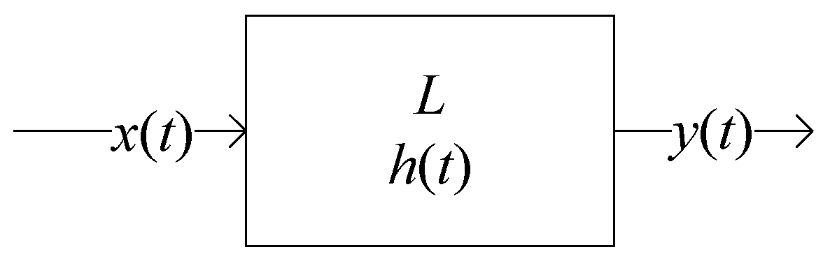
We discuss an application of ${\delta }^{(v)}(t)$ in this section. Denote by h(t) the impulse response of a linear system L (Figure 1). The system response y(t) under the excitation x(t) is acquired by

y(t) = x(t)∗h(t),

(17)

where ∗ stands for the convolution. When $x(t)={\delta }^{(v)}(t),$ we have

$$y(t)={\delta }^{(v)}(t)\ast h(t)=h^{(v)}(t).$$

(18)

The above implies that the system with the impulse response h(t) under the excitation ${\delta }^{(v)}(t)$ equals to the system with the impulse response $h^{(v)}(t)$ under the excitation δ(t) as shown in Figure 2.

Using Theorem 2 and Equation (18), we may write $h^{(v)}(t)$ by

$$h^{(\nu )}(t)={\delta }^{(\nu )}(t)\ast h(t)=\frac{1}{\pi }{\displaystyle \underset{-\infty }{\overset{\infty }{\int }}\left[{\displaystyle \underset{0}{\overset{\infty }{\int }}{\omega }^{\nu }\cos \left(\omega \tau -\frac{\pi \nu }{2}\right)d\omega }\right]h(t-\tau )d\tau }.$$

(19)

Let 0 < H < 1, where H is the Hurst parameter. Let

$$h(t)=\frac{\sqrt{V_H\sin (H\pi )\mathsf{\Gamma }(2H+1)}}{-2\sin \left(\frac{(H-3/2)\pi }{2}\right)\mathsf{\Gamma }\left(H-\frac{1}{2}\right)}\frac{\mathsf{\Gamma }(-H)}{\mathsf{\Gamma }\left(\frac{3}{2}-H\right)}{t}^H,$$

(20)

where

$$V_H=\mathsf{\Gamma }(1-2H)\frac{\cos \pi H}{\pi H}.$$

(21)

The above h(t) is a power function with dependence (Li [34]). According to Equation (10), we have

$$h^{\left(\frac{3}{2}\right)}(t)=\frac{\sqrt{V_H\sin (H\pi )\mathsf{\Gamma }(2H+1)}}{-2\sin \left(\frac{(H-3/2)\pi }{2}\right)\mathsf{\Gamma }\left(H-\frac{1}{2}\right)}{t}^{-\frac{3}{2}+H}.$$

(22)

Let w(t) be the standard white noise. Denote by G(t) the fractional Gaussian noise. Then, under the excitation w(t), the response to a system with the impulse response function h^(1.5)(t) is

$$G(t)=w(t)\ast h^{\left(3/2\right)}(t)=\frac{\sqrt{V_H\sin (H\pi )\mathsf{\Gamma }(2H+1)}}{-2\sin \left(\frac{(H-3/2)\pi }{2}\right)\mathsf{\Gamma }\left(H-\frac{1}{2}\right)}{\displaystyle \underset{-\infty }{\overset{\infty }{\int }}\frac{w(\tau )}{{(t-\tau )}^{\frac{3}{2}-H}}}d\tau .$$

(23)

The above is a new alternative representation of G(t) that was previously reported by Li et al. [35]. To be precise, G(t) may be taken as a response to a system with the impulse response function h^(1.5)(t) under the excitation w(t). An interesting alternative of Equation (23) is given by

$$G(t)=w^{(3/2)}(t)\ast h(t)=\frac{\sqrt{V_H\sin (H\pi )\mathsf{\Gamma }(2H+1)}}{-2\sin \left(\frac{(H-3/2)\pi }{2}\right)\mathsf{\Gamma }\left(H-\frac{1}{2}\right)}\frac{\mathsf{\Gamma }(-H)}{\mathsf{\Gamma }\left(\frac{3}{2}-H\right)}{\displaystyle \underset{-\infty }{\overset{\infty }{\int }}{w}^{(3/2)}(\tau ){(t-\tau )}^H}d\tau .$$

(24)

The above exhibits another new alternative representation of G(t), which may be taken as the response to a system with the impulse response h(t) under the excitation w^(1.5)(t).

5. Conclusions

The results presented in Theorems 1 and 2 are the integral representations of the fractional derivative of the delta function, providing a solution to the tough problem. In addition, we discussed the application of the representation of the fractional derivative of the delta function in representing the fractional Gaussian noise.

References

- Harris, C.M. Shock and Vibration Handbook, 5th ed.; McGraw-Hill: New York, NY, USA, 2002. [Google Scholar]
- Korn, G.A.; Korn, T.M. Mathematical Handbook for Scientists and Engineers; McGraw-Hill: New York, NY, USA, 1961. [Google Scholar]
- Mitra, S.K.; Kaiser, J.F. Handbook for Digital Signal Processing; John Wiley & Sons: Hoboken, NJ, USA, 1993. [Google Scholar]
- Palley, O.M.; Bahizov, Γ.B.; Voroneysk, E.Я. Handbook of Ship Structural Mechanics; Xu, B.H., Xu, X., Xu, M.Q., Eds.; National Defense Industry Publishing House: Beijing, China, 2002. (In Chinese) [Google Scholar]
- Li, M. Three classes of fractional oscillators. Symmetry 2018, 10, 40. [Google Scholar] [CrossRef] [Green Version]
- Li, C. The powers of the Dirac delta function by Caputo fractional derivatives. J. Fract. Calc. Appl. 2016, 7, 12–23. [Google Scholar]
- Dirac, P.A.M. The Principle of Quantum Mechanics; Oxford University Press: Oxford, UK, 1958. [Google Scholar]
- Robinson, E.A. A historical perspective of spectrum estimation. Proc. IEEE 1982, 70, 885–907. [Google Scholar] [CrossRef]
- Walton, J.R. A note on certain asymptotic expressions for the unit-step and Dirac delta functions. SIAM J. Appl. Math. 1976, 31, 304–306. [Google Scholar] [CrossRef]
- Novomestky, F. Asymptotic expressions for the unit-step and Dirac delta functions. SIAM J. Appl. Math. 1974, 27, 521–525. [Google Scholar] [CrossRef]
- Hoskins, R.F. Delta Functions: An Introduction to Generalized Functions; Horwood Pub: Chichester, UK, 2009; pp. 43–46. [Google Scholar]
- Gelfand, I.M.; Vilenkin, K. Generalized Functions; Academic Press: New York, NY, USA, 1964; Volume 1. [Google Scholar]
- Li, C.K.; Li, C.P. Remarks on fractional derivatives of distributions. Tbil. Math. J. 2017, 10, 1–18. [Google Scholar] [CrossRef]
- Makris, N. The fractional derivative of the Dirac delta function and new results on the inverse Laplace transform of irrational functions. arXiv 2020, arXiv:2006.04966. Available online: https://arxiv.org/pdf/2006.04966.pdf (accessed on 17 August 2020).
- Fractional Derivative of Delta Function δ(x). Available online: https://math.stackexchange.com/questions/201656/fractional-derivatives-of-delta-function-delta-x (accessed on 27 August 2020).
- Liouville, J. Memoire sur le theoreme des complementaires. J. Reine Angew. Math. 1834, 11, 1–19. [Google Scholar]
- Ross, B. Fractional Calculus and Its Applications; Lecture Notes in Mathematics; Springer: New York, NY, USA, 1975; Volume 457. [Google Scholar]
- Weyl, H. Bemerkungen zum Begriff des Differentialquotienten gebrochener Ordnung. Vierteljschr Naturforsch. Ges. Zur. 1917, 62, 296–302. [Google Scholar]
- Raina, R.K.; Koul, C.L. On Weyl Fractional Calculus. Proc. Am. Math. Soc. 1979, 73, 188–192. [Google Scholar] [CrossRef]
- Klafter, J.; Lim, S.C.; Metzler, R. Fractional Dynamics: Recent Advances; World Scientific: Singapore, 2012. [Google Scholar]
- Sabatier, J.; Farge, C. Comments on the description and initialization of fractional partial differential equations using Riemann-Liouville’s and Caputo’s definitions. J. Comput. Appl. Math. 2018, 339, 30–39. [Google Scholar] [CrossRef]
- Giusti, A. A comment on some new definitions of fractional derivative. Nonlinear Dyn. 2018, 93, 1757–1763, Addendum in 2018, 94, 1547. [Google Scholar] [CrossRef] [Green Version]
- Hristov, J. Derivatives with non-singular kernels from the Caputo-Fabrizio definition and beyond: Appraising analysis with emphasis on diffusion models. In Frontiers in Fractional Calculus; Bhalekar, S., Ed.; Bentham Science Publishers: Sharjah, UAE, 2017; Volume 1, pp. 270–342. [Google Scholar]
- Khalil, R.; Al Horani, M.; Yousef, A.; Sababheh, M. A new definition of fractional derivative. J. Comput. Appl. Math. 2014, 264, 65–70. [Google Scholar] [CrossRef]
- Gao, G.-H.; Sun, Z.-Z.; Zhang, H.-W. A new fractional numerical differentiation formula to approximate the Caputo fractional derivative and its applications. J. Comput. Phys. 2014, 259, 33–50. [Google Scholar] [CrossRef]
- Zheng, Z.; Zhao, W.; Dai, H. A new definition of fractional derivative. Int. J. NonLinear Mech. 2019, 108, 1–6. [Google Scholar] [CrossRef]
- Atanackovic, T.M.; Pilipovic, S.; Stankovic, B.; Zorica, D. Fractional Calculus with Applications in Mechanics; John Wiley & Sons: Hoboken, NJ, USA, 2014. [Google Scholar]
- Caputo, M.; Fabrizio, M. The kernel of the distributed order fractional derivatives with an application to complex materials. Fractal Fract. 2017, 1, 13. [Google Scholar] [CrossRef] [Green Version]
- Miller, K.S.; Ross, B. An Introduction to the Fractional Calculus and Fractional Differential Equations; John Wiley: Hoboken, NJ, USA, 1993. [Google Scholar]
- Lavoie, J.L.; Osler, T.J.; Tremblay, R. Fractional derivatives and special functions. SIAM Rev. 1976, 18, 240–268. [Google Scholar] [CrossRef]
- Li, C.P.; Zeng, F.H. Numerical Methods for Fractional Calculus; Chapman and Hall/CRC: Boca Raton, FL, USA, 2015. [Google Scholar]
- Li, C.P.; Cai, M. Theory and Numerical Approximations of Fractional Integrals and Derivatives; SIAM: Philadelphia, PA, USA, 2019. [Google Scholar]
- Yang, H.; Guo, J.Y.; Jung, J.-H. Schwartz duality of the Dirac delta function for the Chebyshev collocation approximation to the fractional advection equation. Appl. Math. Lett. 2017, 64, 205–212. [Google Scholar] [CrossRef]
- Li, M. Dependence of a class of non-integer power functions. J. King Saud Univ. (Sci.) 2016, 28, 355–358. [Google Scholar] [CrossRef] [Green Version]
- Li, M.; Sun, X.; Xiao, X. Revisiting fractional Gaussian noise. Phys. A 2019, 514, 56–62. [Google Scholar] [CrossRef]
Figure 1.
Linear system.
Figure 2.
A fractional system resulting from
© 2020 by the author. Licensee MDPI, Basel, Switzerland. This article is an open access article distributed under the terms and conditions of the Creative Commons Attribution (CC BY) license (http://creativecommons.org/licenses/by/4.0/).
Share and Cite
MDPI and ACS Style
Li, M. Integral Representation of Fractional Derivative of Delta Function. Fractal Fract. 2020, 4, 47. https://doi.org/10.3390/fractalfract4030047
AMA Style
Li M. Integral Representation of Fractional Derivative of Delta Function. Fractal and Fractional. 2020; 4(3):47. https://doi.org/10.3390/fractalfract4030047
Chicago/Turabian StyleLi, Ming. 2020. "Integral Representation of Fractional Derivative of Delta Function" Fractal and Fractional 4, no. 3: 47. https://doi.org/10.3390/fractalfract4030047