Fractional Derivatives and Dynamical Systems in Material Instability

Department of Vehicle Elements and Vehicle-Structure Analysis, Budapest University of Technology and Economics, 1111 Budapest, Hungary
†
Current address: Műegyetem rkp. 1–3. H-1111 Budapest, Hungary.
Fractal Fract. 2020, 4(2), 14; https://doi.org/10.3390/fractalfract4020014
Submission received: 28 February 2020
/
Revised: 13 April 2020
/
Accepted: 13 April 2020
/
Published: 16 April 2020
(This article belongs to the Special Issue Fractional Behavior in Nature 2019)
Abstract
:Loss of stability is studied extensively in nonlinear investigations, and classified as generic bifurcations. It requires regularity, being connected with non-locality. Such behavior comes from gradient terms in constitutive equations. Most fractional derivatives are non-local, thus by using them in defining strain, a non-local strain appears. In such a way, various versions of non-localities are obtained by using various types of fractional derivatives. The study aims for constitutive modeling via instability phenomena, that is, by observing the way of loss of stability of material, we can be informed about the proper form of its mathematical model.
1. Introduction
There are materials where tests justify models with fractional order derivatives. Moreover, all fractional derivatives are non-local. Thus, by using strain calculated by fractional derivation of the displacement field, a non-local quantity appears instead of the conventional (local) strain. Fractional calculus appears to be a powerful tool to deal with forms of non-localities. When the term non-locality is used in its original meaning, the value of some quantity in an internal point of the body is determined by the values of other quantities in a whole region around that location.
In material instability problems, like shear band or neck formation [1], the post-critical behavior plays an essential role. Especially for numerical analysis [2], the form and thickness of instability zones should be mesh-independent for a proper material model. Such property implies a generic method of the loss of stability in the sense of dynamical systems theory [3,4]. Thus, the complete mathematical description of the solid continuum (a set of differential equations) should undergo a generic bifurcation. While that model is more or less fixed, the only element of the set of basic equations to be varied is the constitutive equation. Consequently, one should use a constitutive equation, which, by adding the equations of motion and the kinematic equation, forms a system, having generic bifurcation at loss of stability. Conventionally, such constitutive equations are formed by gradient regularization [5], which can also be interpreted as addition of non-locality.
Non-locality is an essential part of continuum physics from the early period of rational mechanics. Two forms are distinguished, the weak and the strong non-localities [6]. The earliest distinction was introduced by Maugin in 1977 at a conference in Warsaw [7]. Weak non-locality concepts that use gradient models could be better referred to as gradient theories of the n-th order [6]. At strong non-locality, constitutive equations become integral expressions over space, perhaps with a more or less rapid attenuation with the distance of the spatial kernel [6]. In a continuum physicist’s point of view, the use of fractional derivatives fits well into the generalization of strong non-locality theory [8].
Weak non-localities can be introduced like Aifantis [5], by adding gradient term(s) to constitutive equations
Term is used in Equation (1) as in [5], to express second "gradient dependence" of material [8]. (Obviously, such an operator is the Laplace operator, ). Gradient effects have several physical interpretation including internal lengths or micro-structural effect theories. Early studies from the 1960s use the notion of polar bodies [9] and couple stress effect and then a gradient of deformation gradient appears, which can be interpreted as a constitutive equation containing a first order strain gradient.
In case of strong non-locality, local stress is determined by the strain in a neighborhood [10]. Similarly to [11], assume that such interval in a uniaxial case is . Then, integration is used to encounter that with attenuation function , which reads
by transforming into the displacement field and assuming attenuation function as
with ,
In [11], one could see how Formula (2) can easily be generalized to Caputo’s fractional derivative. It shows why non-locality is often modeled by using non-local derivatives [12] and then constitutive equations are in the forms of fractional differential equations [13]. This work deals with the consequences of fractional material models in material instability investigations.
The structure of this paper is as follows. Firstly, a short overview of basic fractional calculus is presented, including Euler’s gamma function. A wide range of detailed monographs of that topic is available like [14] or [13] and the reference in them. Secondly, dynamical systems theory is introduced and applied to material instability problems to explain the importance of a property called generic in bifurcation analysis. The most important part is the following section, in which conditions of generic bifurcation behavior are studied for various types of constitutive equations using various fractional derivatives.
2. Elements of Fractional Calculus
2.1. Fractional Integral Operators and Fractional Derivatives
Fractional derivatives are constructed from a fractional order generalization of Cauchy’s integra formula. In such a way, Riemann–Liouville’s fractional integral operator
is defined, where and Euler’s gamma function is an integral of the two most important functions of analysis. These are power function and exponential functions and then
It can also be interpreted as a generalization of factorial to non-integers because, for integer , definition (4) results in being factorial,
Integration in Formula (3) goes from left to right, ; for that reason, it is called the left integral operator. By taking a derivative of the left Riemann–Liouville integral operator, a fractional derivative
can be defined. The usual form of the left Riemann–Liouville derivative is obtained from Formulas (3) and (6)
which is a non-local fractional derivative for interval .
By varying the interval of integral operator in Formula (7) to , the so-called right Riemann–Liouville derivative can be defined as
By changing operators of derivation and integration in Formula (6), left Caputo’s derivative is defined
and then its integro-differential operator formula reads
being the left (non-local) Caputo derivative for interval . Hence, the right Caputo derivative for interval reads
2.2. Symmetric Fractional Derivatives
For most applications in non-local mechanics, fractional derivative
should be a symmetric derivative. For example, such derivative can be constructed from left and right Riemann–Liouville
or Caputo derivatives
or similarly from other types of left and right fractional derivatives. As a famous example in fractional mechanics, a symmetric derivative [15] is presented. Let us start from equivalent forms of the left and right Caputo derivatives like [16]. From (8),
is obtained and (9) is equivalent to
Then, take “asymptotic cases” (, ) and combine them into a symmetric form of Liouville–Caputo derivatives, like
which is closely related to the Riesz potential [15].
2.3. On a Two-Sided Fractional Derivative as Infinite Series
There is a more efficient way to construct symmetric fractional derivatives. Its origin is at Grünwald–Letnikov formulation. For repeated backward differentiation [17]
where
Then, instead of integer , take fractional order difference as an infinite series
where
Now, for , the left- and right-sided Grünwald–Letnikov derivatives are
and a symmetric derivative can be constructed by adding them together. In a similar way, so-called centered derivatives could be defined and even integral forms are available [18]. As a generalized version, in this study, the two-sided fractional derivatives (TSFD) are used as it was introduced by Ortigueira [19]
where . The solution of the eigenvalue – eigenvector problem for differential operator (12) is
and this fact will be used extensively in our stability investigation.
3. A Dynamical Systems Approach of Material Instability
The classical description of continuum mechanics consists of the set of basic equations of continua. In this section, a dynamical system is constructed from these equations and material instability of a state of material is studied as an instability of a solution of that dynamical system.
In the simplest possible case, a uniaxial problem is studied with small deformations. Then, basic equations are
- Cauchy’s equations of motion
- the kinematic equation in rate form
- and the constitutive equation
Note that constitutive Equation (16) is used here in its general form, a function of strain field , stress field , and various derivatives of them. Moreover, in addition to the variables shown in Equation (16), further dependence may and will appear later in this paper. Strain gradient and fractional strain gradient may also be included into the constitutive equation.
Then, by introducing homogeneous perturbations,
and
the linearization of Equations (17) and (18) is satisfied for the perturbations. In that sense, homogeneous perturbation for a uniaxial continuum of length L means that
In mechanics, the case of adiabatic localization [20] may justify the case of infinite length [15], (), especially for material instability problems. Such case assumes that the effect of the boundaries can be eliminated sufficiently far from both ends of a rod, which correlates the experimental observations. Shear bands or necking regions appear generally "in the middle" of a specimen, sufficiently far from both ends.
As it is presented in [21], the eigenvalues and eigenvectors of linearized operator
play the key role in stability and bifurcation analysis. For this reason, the characteristic equation of Formula (22)
should be solved and stability conditions are formed for its solutions in a usual way:
- state of the material is stable, iffor all solutions of Equation (23),
- loss-of-stability happens, when at least for one i,
Two ways of instabilities can be distinguished,
- the static bifurcation , that is,and
- the dynamic bifurcation ,
for non-trivial .
Nonlinear analysis can be performed, if operator defined by Formula (22) has non-trivial critical eigenspace, thus Equation (23) should have a non-trivial solution at . Such case is referred to as generic bifurcation and nonlinearity should be projected to this eigenspace resulting in bifurcation equations [21]. For this reason, the existence and exact determination of are of critical importance. The following section deals with that problem in the case of various constitutive equations.
Characteristic Equation (23) is a partial differential equation, while Formula (22) is a differential operator. Its solution, or its solvability is far from obvious even in the case of integer order derivatives. A kind of simplifying approximation is to restrict the problem to some proper functions. Such functions are harmonics in the so-called periodic perturbation technique [21]. When homogeneous boundary conditions given by Formulas (19)–(21) are taken into consideration, the perturbation frequencies are
4. Bifurcations for Constitutive Equations with Fractional Derivatives
4.1. Constitutive Equation with Non-Local Strain
Firstly, strong non-locality is assumed. In such case, local stress is determined by the strain in a neighborhood [10]. A generalization of such approach is the use of a non-local strain, where, instead of local strain
a non-local one is used, defined by a symmetric fractional derivative
(see Formulas (10)–(12)). In Formula (26), absolute value points out the symmetric nature of derivative. Then, a static bifurcation is studied at non-local strain as in [15].
Let the constitutive equation be the so-called Malvern–Cristescu equation
and let us extend the scope of investigation to dynamic bifurcation too. Now, characteristic Equation (23) has the form
4.1.1. Malvern–Cristescu Constitutive Equation at TSFD
By using TSFD, static bifurcation condition reads Formula (29)
and for all periodic perturbations the critical tangent stiffness is . Here, a kind of lack of generic behavior is that all perturbations are critical. This means that no finite dimensional critical eigenspace can be determined.
For the dynamic bifurcation (condition in Formula (25)), by substituting into Equation (28),
is obtained. Assume that ; then, by substituting Formula (13) into Equation (30), the bifurcation condition is
The next step is to get real and imaginary partition of Equation (31). The real part leads to
while the imaginary part implies
The solution of the “real part” for reads
One might introduce
Then, the imaginary part results
and the solution for the “real part” is
4.1.2. Malvern–Cristescu at Riesz Derivative
To study the dynamic bifurcation of Malvern-Cristescu equation, one should return to Equations (32) and (33). In such case, these are
and
Remark that either or leads to the “classical” coexistent dynamic and static bifurcation case at .
4.1.3. Classical Visco-Elasto-Plastic Case at Riesz Derivative
For a classical visco-elasto-plastic material, . While represents the case of symmetric Riesz derivative [19], Equation (34) implies
and Equation (32) implies
Unfortunately, Formula (40) is the same as the static bifurcation condition, thus such constitutive equation results in non-generic coexistent static and dynamic bifurcations, consequently unavailable for a dynamic stability analysis. Additionally, non-generic behavior appears also in the fact that all periodic perturbations are critical ( all values of can be selected as a critical perturbing frequency).
4.2. Fractional Gradient Material
As an example of strong non-locality, second gradient materials are studied. As it is used by Aifantis [5], a second gradient term should be included into constitutive equations and Formula (1) is obtained. In the Aifantis–Tarasov material model [22], the idea is to use fractional derivative in Formula (1). In uniaxial form, such equation reads
However, non-locality is already involved in Equation (42) and the use of local “fractional” derivatives might even be possible in the sense of non-local mechanics ([23,24]). However, such derivatives are widely criticized [25]; for this reason, TSFD will be used again:
In this case, characteristic Equation (23) reads
Then, for periodic perturbations (selected to be the eigenfunctions of ),
is obtained. Equation (45) can be solved to
By expressing B from Equation (47) as a function of perturbation frequency , its graph is plotted in Figure 2 at .
Dynamic bifurcation study requires adding rate dependence to the constitutive Equation (43)
Then, the characteristic equation is
for eigenfunctions
Equation (50) can be solved for
A necessary condition for dynamic bifurcation is
4.3. Non-Local Strain Gradient Material
In case of a generalization of the classical second gradient dependent material [5], the constitutive equation reads
In material model of Formula (53), both weak (second gradient term) and strong non-localities (fractional strain) are present.
In this case, a critical perturbation can be identified. Then, static bifurcation condition in Formula (24) for periodic perturbations
results in being
Equation (54) implies that
Then, critical perturbation frequency is
and the non-trivial eigenfunction is
5. Conclusions
Stability analysis was performed for non-local materials. Non-locality was modeled by using fractional derivatives. The main aim was to guarantee non-trivial critical eigenfunctions at the loss of stability. Such eigenfunctions play an important role in nonlinear studies because nonlinearities are projected to them to form bifurcation equations. This case is referred to as generic bifurcation. The existence of non-trivial critical eigenfunctions was studied for various non-local constitutive equations.
Two main groups distinguished the strong and the weak types of non-localities. In the case of strongly non-local materials, the introduction of fractional strain via fractional derivative seems to be an obvious generalization of the classical theories. Fractional derivatives here should be non-local and symmetric. The so-called two-sided fractional derivatives by [19] satisfy all these requirements and its special version, the Riesz derivative, was used in all bifurcation investigations.
Constitutive relations were classified as equations with non-local strain and fractional gradient dependent ones. The first type was represented by the Malvern–Cristescu equation and a simplified version of it, called the classical visco-elasto-plastic material. The second group was represented by the fractional gradient material (Aifantis–Tarasov model), its rate dependent version. At the end, the non-local strain gradient material was studied.
The main results are as follows:
- In case of classical visco-elasto-plastic material, no generic nature can be assumed. Both infinite dimensional critical eigenspace and coexistent static and dynamic bifurcations are found. Thus, such equation cannot be used for any nonlinear stability analysis.
- In the case of non-local strain gradient material, both strong and weak non-localities are present in the constitutive equation. The results are the same as the simple second gradient material [21].
Funding
This research received no external funding.
Conflicts of Interest
The author declares no conflicts of interest.
References
- Rice, J.R. The localization of plastic deformation. In Theoretical and Applied Mechanics; Koiter, W.T., Ed.; North-Holland Publ.: Amsterdam, The Netherlands, 1976; pp. 207–220. [Google Scholar]
- De Borst, R.; Sluys, L.J.; Muhlhaus, H.B.; Pamin, J. Fundamental issues in finite element analyses of localization of deformation. Eng. Comput. 1993, 10, 99–121. [Google Scholar]
- Farkas, M. Periodic Motions; Springer: New York, NY, USA, 1994. [Google Scholar]
- Arnold, V.I. Geometrical Methods in the Theory of Ordinary Differential Equations; Springer: New York, NY, USA, 1983. [Google Scholar]
- Aifantis, E.C. On the role of gradients in the localization of deformation and fracture. Int. J. Eng. Sci. 1992, 30, 1279–1299. [Google Scholar] [CrossRef]
- Maugin, G.A.; Metrikine, A.V. Mechanics of Generalized Continua; Springer: New York, NY, USA, 2010. [Google Scholar]
- Maugin, G.A. Nonlocal theories or gradient-type theories: a matter of convenience? Arch. Mech. 1979, 31, 15–26. [Google Scholar]
- Maugin, G.A. Non-Classical Continuum Mechanics; Springer Nature: Singapore, 2017. [Google Scholar]
- Toupin, R.A. Theories of elasticity with couple-stresses. Arch. Ration. Mech. and Anal. 1962, 17, 85–112. [Google Scholar] [CrossRef]
- Eringen, A.C. Nonlocal Continuum Field Theories; Springer: New York, NY, USA, 2002. [Google Scholar]
- Carpinteri, A.; Cornetti, P.; Sapora, A. A fractional calculus approach to nonlocal elasticity. Eur. J. Phys. 2011, 193, 193–204. [Google Scholar] [CrossRef]
- Lazopoulos, K.A. Non-local continuum mechanics and fractional calculus. Mech. Res. Commun. 2006, 33, 753–757. [Google Scholar] [CrossRef]
- Diethelm, K. The Analysis of Fractional Differential Equations; Springer: New York, NY, USA, 2010. [Google Scholar]
- Podlubny, I. Fractional Differential Equations; Academic Press: San Diego, CA, USA, 1999. [Google Scholar]
- Atanackovic, T.M.; Stankovic, B. Generalized wave equation in nonlocal elasticity. Acta Mech. 2009, 208, 1–10. [Google Scholar] [CrossRef]
- Samko, S.G.; Kilbas, A.A.; Marichev, O.I. Fractional Integrals and Derivatives; Gordon and Breach: Amsterdam, The Netherlands, 1993. [Google Scholar]
- Tarasov, V.E. Fractional Dynamics; Springer-Verlag: Berlin/Heidelberg, Germany, 2010. [Google Scholar]
- Ortigueira, M.D. Riesz potential operators and inverses via fractional centred derivatives. Int. J. Math. Math. Sci. 2006, 48391. [Google Scholar] [CrossRef]
- Ortigueira, M.D. Two-sided and regularised Riesz-Feller derivatives. Math. Meth. Appl. Sci. 2019, 1–13. [Google Scholar] [CrossRef]
- Dobovsek, I. Adiabatic material instabilities in rate-independent solids. Arch. Mech. 1994, 46, 893–936. [Google Scholar]
- Béda, P.B. Dynamic systems, rate and gradient effects in material instability. Int. J. Mech. Sci. 2000, 42, 2101–2114. [Google Scholar] [CrossRef]
- Tarasov, V.E.; Aifantis, E.C. Non-standard extensions of gradient elasticity: Fractional non- locality, memory and fractality. Commun. Nonlinear Sci. Numer. Simulat. 2015, 22, 197–227. [Google Scholar] [CrossRef] [Green Version]
- Khalil, R.; Horani, M.A.; Yousef, A.; Sababheh, M. A new definition of fractional derivative. J. Comput. Appl. Math. 2014, 264, 65–70. [Google Scholar] [CrossRef]
- Rahimi, Z.; Sumelka, W.; Baleanu, D. A mechanical model based on conformal strain energy and its application to bending and buckling of nanobeam structures. ASME J. Comput. Nonlinear Dynam. 2019, 14, 061004. [Google Scholar] [CrossRef]
- Tarasov, V.E. No nonlocality. No fractional derivative. Commun. Nonl. Sci. Numer. Simul. 2018, 62, 157–163. [Google Scholar] [CrossRef] [Green Version]
Figure 1.
Dynamic bifurcation of Malvern–Cristescu material: tangent stiffness as function of at various orders of derivative .
Figure 1.
Dynamic bifurcation of Malvern–Cristescu material: tangent stiffness as function of at various orders of derivative .

Figure 2.
Static bifurcation of Aifantis–Tarasov material: critical tangent stiffness as function of at various orders of derivative .
Figure 2.
Static bifurcation of Aifantis–Tarasov material: critical tangent stiffness as function of at various orders of derivative .

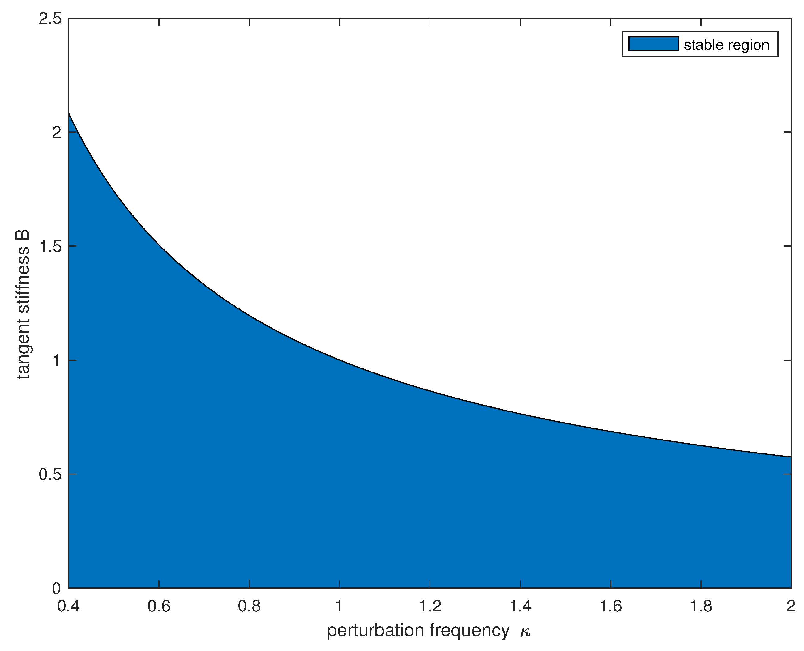
Figure 3.
Stability chart for .

© 2020 by the author. Licensee MDPI, Basel, Switzerland. This article is an open access article distributed under the terms and conditions of the Creative Commons Attribution (CC BY) license (http://creativecommons.org/licenses/by/4.0/).
Share and Cite
MDPI and ACS Style
Béda, P.B. Fractional Derivatives and Dynamical Systems in Material Instability. Fractal Fract. 2020, 4, 14. https://doi.org/10.3390/fractalfract4020014
AMA Style
Béda PB. Fractional Derivatives and Dynamical Systems in Material Instability. Fractal and Fractional. 2020; 4(2):14. https://doi.org/10.3390/fractalfract4020014
Chicago/Turabian StyleBéda, Peter B. 2020. "Fractional Derivatives and Dynamical Systems in Material Instability" Fractal and Fractional 4, no. 2: 14. https://doi.org/10.3390/fractalfract4020014