Article

A Novel Method for Solutions of Fourth-Order Fractional Boundary Value Problems

1
Department of Mathematics, Art and Science Faculty, Siirt University, 56100 Siirt, Turkey
2
Department of Mathematics, Faculty of Education, Siirt University, 56100 Siirt, Turkey
*
Author to whom correspondence should be addressed.
Fractal Fract. 2019, 3(2), 33; https://doi.org/10.3390/fractalfract3020033
Submission received: 24 May 2019 / Revised: 16 June 2019 / Accepted: 17 June 2019 / Published: 18 June 2019

Abstract

:
In this paper, we find the solutions of fourth order fractional boundary value problems by using the reproducing kernel Hilbert space method. Firstly, the reproducing kernel Hilbert space method is introduced and then the method is applied to this kind problems. The experiments are discussed and the approximate solutions are obtained to be more correct compared to the other obtained results in the literature.

1. Introduction

Boundary value problems come into view in many areas of science and engineering [1]. Many numerical methods have been presented for solving boundary value problems recently [2]. Wazwaz [3] has presented a modified decomposition method for investigating a special class of fourth order boundary value problems. The series solution of fourth order boundary value problems has been investigated by Adomian decomposition method in [4]. The differential transform method was implemented in [5] for series solution of fourth order boundary value problems. The approximate solution of two-point fourth order boundary value problems utilizing non-polynomial quintic spline functions have been given in [6,7]. Lodhi and Mishra [8] have enhanced a numerical method for solving fourth order boundary value problems utilizing quintic B-spline functions. A numerical technique depending on non-polynomial spline functions has been applied in [9] for the numerical solution of self-adjoint singularly perturbed fourth order boundary value problems. Akram and Amin [10] have applied quintic spline collocation method for approximate solution of singularly perturbed fourth order boundary value problems.
Fractional order boundary value problems have taken much interest by many investigators due to their implementations in many areas of science and engineering. Recently, much attentions have been given to investigate fractional order differential equations [11].
We take into consideration the following fourth order fractional boundary value problems arising in plate deflection theory by the reproducing kernel Hilbert space method.
u ( 4 ) ( z ) + D γ p ( z ) u ( z ) = g ( z ) , z [ a , b ] ,
subject to the end conditions
u ( a ) a 1 = u ( b ) a 2 = u ( a ) b 1 = u ( b ) b 2 = 0 .
where a i s , b i s , ( i = 1 , 2 ) are real constants and 0 γ 1 . p ( z ) and g ( z ) are continuous on the [ a , b ] .
Let H be a Hilbert space of functions on some set X, which every point consideration at points in X are continuous in the norm of H. Such space H, can be given by a positive definite kernel. This fact is first presented by Aronszajn [12]. These Hilbert spaces are called the reproducing kernel Hilbert spaces [13].
Arqub [14] has found the approximate solutions of DASs with nonclassical boundary conditions using a novel reproducing kernel algorithm. Arqub [15] has investigated the reproducing kernel algorithm for handling differential algebraic systems of ordinary differential equations. Arqub [16] has applied a fitted reproducing kernel Hilbert space method for the solutions of some certain classes of time-fractional partial differential equations subject to initial and Neumann boundary conditions. Azarnavid et al. [17] have investigated the Picard-reproducing kernel Hilbert space method for solving generalized singular nonlinear Lane–Emden type equations. Azarnavid et al. [18] have found multiplicity results by shooting reproducing kernel Hilbert space method for the catalytic reaction in a flat particle. Azarnavid et al. [19] have used an iterative kernel based method for fourth order nonlinear equation with nonlinear boundary condition.
We arrange the paper as: The main notions of fractional calculus are given in Section 2. The reproducing kernel Hilbert space method for fourth-order fractional order differential equations is presented in Section 3. The numerical results and discussions are presented in Section 4. The conclusion is presented in the last section.

2. Preliminaries and Notations

We give some definitions of fractional calculus in this section. There are many definitions of fractional derivatives. The definitions of Riemann–Liouville fractional integral and Caputo’s fractional derivative are presented as [17]:
Definition 1.
The Riemann–Liouville left and right fractional integral of order γ > 0 is given as [11]:
I a + γ u ( z ) = 1 Γ ( γ ) a z ( z τ ) γ 1 u ( τ ) d τ , m 1 < γ m , m N ,
and
I b γ u ( z ) = 1 Γ ( γ ) b z ( z τ ) γ 1 u ( τ ) d τ , m 1 < γ m , m N .
where Γ defines the Gamma function.
Definition 2.
The Riemann–Liouville fractional derivative of order γ > 0 is presented as [11]:
D a γ u ( z ) = 1 Γ ( m γ ) d m d z m a z ( z τ ) m γ 1 u ( τ ) d τ , m 1 < γ m , m N .
Definition 3.
The Caputo’s fractional derivative of order γ > 0 is presented as [11]:
D a γ u ( z ) = 1 Γ ( m γ ) a z ( z τ ) m α 1 d m u ( τ ) d τ m d τ , m 1 < α m , m N .
Lemma 1.
Assume that f and g are analytic functions on ( a h , a + h ) and let 0 < γ 1 . Then we have [11]:
D a γ [ f ( z ) g ( z ) ] = ( z a ) γ Γ ( 1 γ ) g ( a ) ( f ( z ) f ( a ) ) + ( D a α g ( z ) ) f ( z ) + l = 1 α l ( I a 1 α g ( z ) ) D a l f ( z ) .

3. Reproducing Kernel Hilbert Space Method

We will construct reproducing kernel Hilbert spaces to solve the problem.
Definition 4.
V 2 1 [ 0 , 1 ] is the first reproducing kernel Hilbert space that we need.
V 2 1 [ 0 , 1 ] = { r A C [ 0 , 1 ] : r L 2 [ 0 , 1 ] } .
The inner product and norm for this reproducing kernel Hilbert space are defined by:
r , q V 2 1 = r ( 0 ) q ( 0 ) + 0 1 r ( z ) q ( z ) d z , r , q V 2 1 [ 0 , 1 ]
and
r V 2 1 = r , r V 2 1 , r V 2 1 [ 0 , 1 ] .
Lemma 2.
The reproducing kernel function U z of V 2 1 [ 0 , 1 ] is obtained as:
U t ( z ) = 1 + z , z t , 1 + t , z > t .
Definition 5.
We construct the reproducing kernel Hilbert space V 2 5 [ 0 , 1 ] as:
V 2 5 [ 0 , 1 ] = { r A C [ 0 , 1 ] : r , r , r , r ( 4 ) A C [ 0 , 1 ] , r ( 5 ) L 2 [ 0 , 1 ] , r ( 0 ) = r ( 1 ) = r ( 0 ) = r ( 1 ) = 0 } .
The inner product and the norm for this special Hilbert space is defined as:
r , q V 2 5 = i = 0 4 r ( i ) ( 0 ) q ( i ) ( 0 ) + 0 1 r ( 5 ) ( z ) q ( 5 ) ( z ) d z , r , q V 2 5 [ 0 , 1 ]
and
r V 2 5 = r , r V 2 5 , r V 2 5 [ 0 , 1 ] .
Theorem 1.
We obtain the reproducing kernel function for the reproducing kernel Hilbert space V 2 5 [ 0 , 1 ] by:
A y ( x ) = a y ( x ) , x y , b y ( x ) , x > y .
where,
a y ( x ) = x 9 362880 + 635131 x 6 y 4 28582381440 + 11 x 6 y 9 142911907200 11 x 6 y 8 15879100800 + x 7 y 2 10080 + 231 x 6 y 8270365 105619 x 7 y 7 3001150051200 + 91723 x 7 y 6 428735721600 + 23 x 5 y 9 31758201600 88249 x 7 y 5 1442911907200 88249 x 7 y 4 28582381440 91723 x 7 y 3 3572797680 193 x 7 y 9 1000383350400 + 193 x 7 y 8 111153705600 579 x 7 y 8270365 2969 x 8 y 66692223360 + 13 x 8 y 9 190549209600 13 x 8 y 8 21172134400 + 193 x 8 y 7 111153705600 11 x 8 y 6 15879100800 69 x 8 y 5 10586067200 69 x 8 y 4 2117213440 + 11 x 8 y 3 132325840 13 x 9 y 9 1714942886400 + 13 x 9 y 8 190549209600 193 x 9 y 7 1000383350400 + 11 x 9 y 6 142911907200 + 23 x 9 y 5 31758201600 635131 x 3 y 4 238186512 + 23 x 9 y 4 6351640320 11 x 9 y 3 1190932560 91 x 9 y 33081460 + 2969 x y 1654073 127013 x 6 y 3 2381865120 91 x y 9 33081460 + 819 x y 8 33081460 579 x y 7 8270365 + 231 x y 6 8270365 + 635131 x 6 y 5 142911907200 + 4347 x y 5 16540730 + 4347 x y 4 3308146 5544 x y 3 1654073 + 127013 x 3 y 3 19848876 636517 x 6 y 6 428735721600 91723 x 3 y 7 3572797680 + 636517 x 3 y 6 3572797680 635131 x 3 y 5 1190932560 635131 x 5 y 3 1190932560 11 x 3 y 9 1190932560 + 11 x 3 y 8 132325840 5544 x 3 y 1654073 222389 x 4 y 4 158791008 + 91723 x 6 y 7 428735721600 88249 x 4 y 7 28582381440 + 635131 x 4 y 6 28582381440 319739 x 4 y 5 4763730240 635131 x 4 y 3 238186512 + 23 x 4 y 9 6351640320 69 x 4 y 8 2117213440 + 4347 x 4 y 3308146 + 222389 x 5 y 4 793955040 + 4347 x 5 y 16540730 88249 x 5 y 7 142911907200 + 635131 x 5 y 6 142911907200 319739 x 5 y 5 23818651200 69 x 5 y 8 10586067200 .
The reproducing kernel function A y ( x ) is symmetric. Therefore, when exchange x and y in a y ( x ) , we will obtain b y ( x ) .
Proof. 
We have
r , A y V 2 5 = i = 0 4 A y ( i ) ( 0 ) r ( i ) ( 0 ) + 0 1 A y ( 5 ) ( z ) r ( 5 ) ( z ) d z ,
by Definition 5. We obtain
r , A y V 2 5 = A y ( 0 ) r ( 0 ) + A y ( 0 ) r ( 0 ) + A y ( 0 ) r ( 0 ) + A y ( 3 ) ( 0 ) r ( 0 ) + A y ( 4 ) ( 0 ) r ( 4 ) ( 0 ) + A y ( 5 ) ( 1 ) r ( 4 ) ( 1 ) A y ( 5 ) ( 0 ) r ( 4 ) ( 0 ) A y ( 6 ) ( 1 ) r ( 3 ) ( 1 ) + A y ( 6 ) ( 0 ) r ( 3 ) ( 0 ) + A y ( 7 ) ( 1 ) r ( 1 ) A y ( 7 ) ( 0 ) r ( 0 ) A y ( 8 ) ( 1 ) r ( 1 ) + A y ( 8 ) ( 0 ) r ( 0 ) + 0 1 A y ( 9 ) ( z ) r ( z ) d z ,
by integration by parts. Since r ( 0 ) = r ( 1 ) = r ( 0 ) = r ( 1 ) = 0 , we get
r , A y V 2 5 = A y ( 0 ) r ( 0 ) + A y ( 3 ) ( 0 ) r ( 3 ) ( 0 ) + A y ( 4 ) ( 0 ) r ( 4 ) ( 0 ) + A y ( 5 ) ( 1 ) r ( 4 ) ( 1 ) A y ( 5 ) ( 0 ) r ( 4 ) ( 0 ) A y ( 6 ) ( 1 ) r ( 3 ) ( 1 ) + A y ( 6 ) ( 0 ) r ( 3 ) ( 0 ) A y ( 8 ) ( 1 ) r ( 1 ) + A y ( 8 ) ( 0 ) r ( 0 ) + 0 1 A y ( 9 ) ( z ) r ( z ) d z .
Since
A y ( 5 ) ( 1 ) = A y ( 6 ) ( 1 ) = A y ( 8 ) ( 1 ) = 0 ,
we get
r , A y V 2 5 = A y ( 0 ) r ( 0 ) + A y ( 3 ) ( 0 ) r ( 3 ) ( 0 ) + A y ( 4 ) ( 0 ) r ( 4 ) ( 0 ) A y ( 5 ) ( 0 ) r ( 4 ) ( 0 ) + A y ( 6 ) ( 0 ) r ( 3 ) ( 0 ) + A y ( 8 ) ( 0 ) r ( 0 ) + 0 1 A y ( 9 ) ( z ) r ( z ) d z .
We have
A y ( 0 ) = 2969 y 1654073 + 4347 y 4 3308146 91 y 9 33081460 + 819 y 8 33081460 + 4347 y 5 16540730 5544 y 3 1654073 579 y 7 8270365 + 231 y 6 8270365 ,
A y ( 3 ) ( 0 ) = 33264 y 1654073 635131 y 4 39697752 11 y 9 198488760 + 33 y 8 66162920 635131 y 5 198488760 + 127013 y 3 3308146 91723 y 7 595466280 + 636517 y 6 595466280 ,
A y ( 4 ) ( 0 ) = 52164 y 1654073 + 222389 y 4 6616292 + 23 y 9 264651680 207 y 8 264651680 319739 y 5 198488760 635131 y 3 9924438 88249 y 7 1190932560 + 635131 y 6 1190932560 ,
A y ( 5 ) ( 0 ) = 52164 y 1654073 + 222389 y 4 6616292 + 23 y 9 264651680 207 y 8 264651680 319739 y 5 198488760 635131 y 3 9924438 88249 y 7 1190932560 + 635131 y 6 1190932560 ,
A y ( 6 ) ( 0 ) = 33264 y 1654073 + 635131 y 4 39697752 + 11 y 9 198488760 33 y 8 66162920 + 635131 y 5 198488760 127013 y 3 3308146 + 91723 y 7 595466280 636517 y 6 595466280 ,
A y ( 8 ) ( 0 ) = 2969 y 1654073 4347 y 4 3308146 + 91 y 9 33081460 819 y 8 33081460 4347 y 5 16540730 + 5544 y 3 1654073 + 579 y 7 8270365 231 y 6 8270365 .
Therefore, we reach
r , A y V 2 5 = 0 y A y ( 9 ) ( z ) r ( z ) d z + y 1 A y ( 9 ) ( z ) r ( z ) d z .
We have
A y ( 9 ) ( z ) = 1 + k ( y ) , z < y , k ( y ) , z > y .
where
k ( y ) = 819 y 8 33081460 1651104 y 1654073 + 4347 y 5 165540730 + 4347 y 4 3308146 91 y 9 33081460 5544 y 3 1654073 579 y 7 8270365 + 231 y 6 8270365 .
Therefore, we find
r , A y V 2 5 = 0 y ( 1 + k ( y ) ) r ( z ) d z + y 1 ( k ( y ) ) r ( z ) d z ,
r , A y V 2 5 = ( 1 + k ( y ) ) ( r ( y ) r ( 0 ) ) + k ( y ) ( r ( 1 ) r ( y ) ) ,
r , A y V 2 5 = r ( y ) .
Thus, the proof is completed. □
We investigate the solutions of the problem (1) and (2) in the reproducing kernel Hilbert space V 2 5 [ 0 , 1 ] . We need to homogenize the conditions to apply the reproducing kernel Hilbert space method. We use the following transformation to homogenize these conditions.
v ( z ) = u ( z ) f ( z )
where
f ( z ) = a 2 b b 1 + 2 a 2 b b 2 a 2 z b 1 2 a 2 z b 2 2 a b 2 b 1 6 ( a b ) a b 2 b 2 + 2 a b z b 1 2 a z b 2 + 3 a z 2 b 2 + 2 b 2 z b 1 6 ( a b ) + z b 2 b 2 3 b z 2 b 1 + z 3 b 1 z 3 b 2 + 6 a a 2 6 ( a b ) 6 b a 1 + 6 z a 1 6 z a 2 6 ( a b ) .
After using the above transformation we obtain the following problem:
H v = v ( 4 ) ( z ) + D γ p ( z ) v ( z ) = M ( z ) , z [ a , b ] ,
subject to the end conditions
v ( a ) = v ( b ) = v ( a ) = v ( b ) = 0
where
M ( z ) = g ( z ) D γ p ( z ) f ( z ) .
Lemma 3.
H is a bounded linear operator.
Proof. 
We will show
H v V 2 1 [ 0 , 1 ] 2 P v V 2 5 [ 0 , 1 ] 2 ,
where P is a positive constant. We know
H v V 2 1 [ 0 , 1 ] 2 = H v , H v V 2 1 [ 0 , 1 ] = H v ( 0 ) 2 + 0 1 H v ( z ) 2 d z .
We obtain
v ( y ) = v ( · ) , A y ( · ) V 2 5 [ 0 , 1 ]
and
H v ( y ) = v ( · ) , H A y ( · ) V 2 5 [ 0 , 1 ] .
Therefore, we reach
H v v V 2 5 [ 0 , 1 ] H A y V 2 5 [ 0 , 1 ] = P 1 v V 2 5 [ 0 , 1 ] .
Thus, we acquire
H v ( 0 ) 2 P 1 2 v V 2 5 [ 0 , 1 ] 2 .
Since
( H v ) ( z ) = v ( · ) , ( H A y ) ( · ) V 2 5 [ 0 , 1 ] ,
we obtain
( H v ) v E 2 5 [ 0 , 1 ] ( H A y ) E 2 5 [ 0 , 1 ] = P 2 v V 2 5 [ 0 , 1 ] .
Then, we find
H v 2 P 2 2 v V 2 5 [ 0 , 1 ] 2 .
At last we obtain
H v V 2 1 [ 0 , 1 ] 2 = H v ( 0 ) 2 + 0 1 ( H v ) ( z ) 2 d z ( P 1 2 + P 2 2 ) v V 2 5 [ 0 , 1 ] 2 ,
where P = P 1 2 + P 2 2 is a positive constant. This completes the proof. □
We construct a i ( z ) = U z i ( z ) and ψ i ( z ) = H * a i ( z ) , where H * is conjugate operator of H. The orthonormal system ψ ^ i ( z ) i = 1 of E 2 5 [ 0 , 1 ] can be obtained by Gram–Schmidt orthogonalization operation of { ψ i ( z ) } i = 1 ,
ψ ^ i ( z ) = k = 1 i β i k ψ k ( z ) , ( β i i > 0 , i = 1 , 2 , ) .
Theorem 2.
If v ( z ) is the exact solution of (8) and (9), then we obtain
v ( z ) = i = 1 k = 1 i β i k M ( z k ) ψ ^ i ( z ) .
where { z i } i = 1 is dense in [ 0 , 1 ] .
Proof. 
We prove this theorem by using the reproducing property, the features of adjoint operator and the complete system as:
v ( z ) = i = 1 v ( z ) , ψ ^ i ( z ) V 2 5 [ 0 , 1 ] ψ ^ i ( z ) = i = 1 k = 1 i β i k v ( z ) , ψ k ( z ) V 2 5 [ 0 , 1 ] ψ ^ i ( z ) = i = 1 k = 1 i β i k v ( z ) , H * a k ( z ) V 2 5 [ 0 , 1 ] ψ ^ i ( z ) = i = 1 k = 1 i β i k H v ( z ) , a k ( z ) V 2 1 [ 0 , 1 ] ψ ^ i ( z ) = i = 1 k = 1 i β i k M ( z ) , U z k V 2 1 [ 0 , 1 ] ψ ^ i ( z ) = i = 1 k = 1 i β i k U ( z k ) ψ ^ i ( z ) .
This completes the proof. □
The approximate solution v n ( z ) can be obtained as:
v n ( z ) = i = 1 n k = 1 i β i k M ( z k ) ψ ^ i ( z ) .

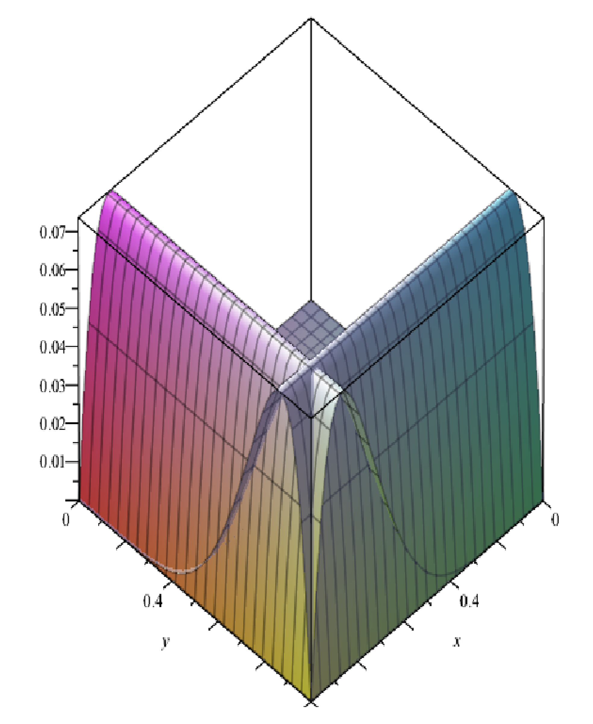
4. Numerical Experiments

Two test examples have been taken into consideration to demonstrate the accuracy of the reproducing kernel Hilbert space method in this section. The numerical simulation has been executed in MAPLE 18.
Example 1.
We consider the fourth order fractional boundary value problem as [17]:
u ( 4 ) ( z ) + 0.05 D γ u ( z ) = g ( z ) , z [ 0 , 1 ] ,
with the boundary conditions
u ( 0 ) = 0 , u ( 1 ) = 0 , u ( 0 ) = 0 , u ( 1 ) = 8 .
We have the exact solution of the problem as z 4 ( z 1 ) .
The absolute errors for different values of γ applying the reproducing kernel Hilbert space method are given in the Table 1. Figure 1, Figure 2 and Figure 3 demonstrate the approximate and exact solution for γ = 1.0 and γ = 0.99 .
Example 2.
We take into consideration the following fourth order fractional boundary value problem [17]:
u ( 4 ) ( z ) + D γ z u ( z ) = g ( z ) , z [ 0 , 1 ] ,
with the boundary conditions
u ( 0 ) = 0 , u ( 1 ) = 0 , u ( 0 ) = 0 , u ( 1 ) = 26 ( γ 1 ) .
We have the exact solution of the problem as z 6 ( z γ z 2 γ ) . The absolute errors applying the reproducing kernel Hilbert space method are presented in the Table 2. Figure 4 and Figure 5 show numerical solutions for γ = 0.3 .

5. Conclusions

We studied the approximate solution of the fourth order fractional boundary value problems in this paper. We applied the reproducing kernel Hilbert space method to our problem. We demonstrated our results by tables and figures. We proved the accuracy of the reproducing kernel Hilbert space method for solutions of fourth order fractional differential equations.

Author Contributions

A.A. and E.K.A. conceived and designed the experiments; A.A. performed the experiments; A.A. and E.K.A. analyzed the data; E.K.A. contributed reagents/materials/analysis tools; A.A. wrote the paper.

Acknowledgments

This work was supported by project 2018-SİUEĞT- 044 .

Conflicts of Interest

The authors declare no conflict of interest.

References

  1. Hajji, M.A.; Al-Khaled, K. Numerical methods for nonlinear fourth-order boundary value problems with applications. Int. J. Comput. Math. 2008, 85, 83–104. [Google Scholar] [CrossRef]
  2. Dehghan, M.; Lakestani, M. Numerical solution of nonlinear system of second-order boundary value problems using cubic B-spline scaling functions. Int. J. Comput. Math. 2008, 85, 1455–1461. [Google Scholar] [CrossRef]
  3. Wazwaz, A.M. The numerical solution of special fourth-order boundary value problems by the modified decomposition method. Int. J. Comput. Math. 2002, 79, 345–356. [Google Scholar] [CrossRef]
  4. Momani, S.; Moadi, K. A reliable algorithm for solving fourth-order boundary value problems. J. Appl. Math. Comput. 2006, 22, 185–197. [Google Scholar] [CrossRef]
  5. Ertürk, V.S.; Momani, S. Comparing numerical methods for solving fourth-order boundary value problems. Appl. Math. Comput. 2007, 188, 1963–1968. [Google Scholar] [CrossRef]
  6. Ramadan, M.; Lashien, I.; Zahra, W. Quintic nonpolynomial spline solutions for fourth order two-point boundary value problem. Commun. Nonlinear Sci. Numer. Simul. 2009, 14, 1105–1114. [Google Scholar] [CrossRef]
  7. Srivastava, P.K.; Kumar, M.; Mohapatra, R. Solution of fourth order boundary value problems by numerical algorithms based on nonpolynomial quintic splines. J. Numer. Math. Stoch. 2012, 4, 13–25. [Google Scholar]
  8. Lodhi, R.K.; Mishra, H.K. Solution of a class of fourth order singular singularly perturbed boundary value problems by quintic b-spline method. J. Niger. Math. Soc. 2016, 35, 257–265. [Google Scholar] [CrossRef]
  9. Lodhi, R.K.; Mishra, H.K. Computational approach for fourth-order self-adjoint singularly perturbed boundary value problems via non-polynomial quintic spline. Iran. J. Sci. Technol. Trans. A Sci. 2016, 42, 1–8. [Google Scholar] [CrossRef]
  10. Akram, G.; Amin, N. Solution of a fourth order singularly perturbed boundary value problem using quintic spline. Proc. Int. Math. Forum 2012, 7, 2179–2190. [Google Scholar]
  11. Khalid, N.; Abbas, M.; Iqbal, M.K. Non-polynomial quintic spline for solving fourth-order fractional boundary value problems involving product terms. Appl. Math. Comput. 2019, 349, 393–407. [Google Scholar] [CrossRef]
  12. Aronszajn, N. Theory of reproducing kernels. Trans. Am. Math. Soc. 1950, 68, 337–404. [Google Scholar] [CrossRef]
  13. Sababe, S.H.; Ebadian, A. Some Properties of Reproducing Kernel Banach and Hilbert Spaces. SCMA 2018, 12, 167–177. [Google Scholar]
  14. Arqub, O.A. Approximate solutions of DASs with nonclassical boundary conditions using novel reproducing kernel algorithm. Fundamenta Informaticae 2016, 146, 231–254. [Google Scholar] [CrossRef]
  15. Arqub, O.A. The reproducing kernel algorithm for handling differential algebraic systems of ordinary differential equations. Math. Methods Appl. Sci. 2016, 39, 4549–4562. [Google Scholar] [CrossRef]
  16. Arqub, O.A. Fitted reproducing kernel Hilbert space method for the solutions of some certain classes of time-fractional partial differential equations subject to initial and Neumann boundary conditions. Comput. Math. Appl. 2017, 73, 1243–1261. [Google Scholar] [CrossRef]
  17. Azarnavid, B.; Parvaneh, F.; Abbasbandy, S. Picard-reproducing Kernel Hilbert space method for solving generalized singular nonlinear Lane–Emden type equations. Math. Model. Anal. 2015, 20, 754–767. [Google Scholar] [CrossRef]
  18. Azarnavid, B.; Shivanian, E.; Parand, K.; Soudabeh, N. Multiplicity results by shooting reproducing kernel Hilbert space method for the catalytic reaction in a flat particle. J. Theor. Comput. Chem. 2018, 17, 1850020. [Google Scholar] [CrossRef]
  19. Azarnavid, B.; Parand, K.; Abbasbandy, S. An iterative kernel based method for fourth order nonlinear equation with nonlinear boundary condition. Commun. Nonlinear Sci. Numer. Simul. 2018, 59, 544–552. [Google Scholar] [CrossRef]
Figure 1. Exact Solutions and Approximate Solutions of Example 1 for γ = 1 .
Fractalfract 03 00033 g001
Figure 2. Exact Solutions and Approximate Solutions of Example 1 for γ = 0.99 .
Fractalfract 03 00033 g002
Figure 3. Exact Solutions and Approximate Solutions of Example 1 for γ = 0.99 .
Fractalfract 03 00033 g003
Figure 4. Exact Solutions and Approximate Solutions of Example 2 for α = 0.3 .
Fractalfract 03 00033 g004
Figure 5. Exact Solutions and Approximate Solutions of Example 2 for γ = 0.3 .
Fractalfract 03 00033 g005
Table 1. Absolute errors for Example 1.
x γ = 0.99 γ = 1.0
0.0 0.000000000000000 0.000000000000000
0.1 1.172251330 × 10 4 1.079370100 × 10 4
0.2 2.050389600 × 10 4 1.892279000 × 10 4
0.3 2.501585000 × 10 4 2.301822740 × 10 4
0.4 2.502148300 × 10 4 2.286283000 × 10 4
0.5 2.134363900 × 10 4 1.922819800 × 10 4
0.6 1.537822000 × 10 4 1.353536000 × 10 4
0.7 8.948229000 × 10 5 7.512914000 × 10 5
0.8 3.720321000 × 10 5 2.799920000 × 10 5
0.9 7.854290000 × 10 6 3.736680000 × 10 6
1.0 1.591755364 × 10 8 4.209367700 × 10 7
Table 2. Absolute errors for Example 2.
x γ = 0.3
0.0 1.542329002 × 10 11
0.1 1.509810086 × 10 4
0.2 2.928833663 × 10 4
0.3 4.165814337 × 10 4
0.4 5.106740380 × 10 4
0.5 5.655431300 × 10 4
0.6 5.714676400 × 10 4
0.7 5.202103100 × 10 4
0.8 4.058811200 × 10 4
0.9 2.300090700 × 10 4
1.0 2.085180231 × 10 7

