Integral Representations and Algebraic Decompositions of the Fox-Wright Type of Special Functions

Abstract

The manuscript surveys the special functions of the Fox-Wright type. These functions are generalizations of the hypergeometric functions. Notable representatives of the type are the Mittag-Leffler functions and the Wright function. The integral representations of such functions are given and the conditions under which these function can be represented by simpler functions are demonstrated. The connection with generalized Erdélyi-Kober fractional differential and integral operators is demonstrated and discussed.

1. Introduction

This paper is concerned with integral representations of the Fox-Wright functions and their relationship to fractional calculus. The first characteristic exemplar of this function family has been introduced by E. M. Wright, who generalized the concept in a series of papers in 1930s. The Fox-Wright special functions are very general mathematical objects, which have broad applications in mathematical physics, notably in descriptions of wave phenomena, heat and mass transfer. They encompass the generalized hypergeometric functions ${}_p{F}_q$ and are related to the family of the Bessel functions.

The conditions for existence of the generalized Wright function together with its representation in terms of the Mellin-Barnes integral and of the H-function can be found in [1]. Fox-Wright functions encompass other important families of functions, such as the the Mittag-Leffler functions (surveys in [2,3]). The Mittag-Leffler function in turn expresses the solution of fractional order integral or fractional order differential equations. It has applications in the theory of random walks, Levy flights, superdiffusive transport, among others. Another important example is the M-Wright function, which expresses the fundamental solution of the time-fractional diffusion-wave equation [4]. A recent survey about the properties of the function can be found in [5].

The objective of the present paper is to give a self-contained treatment of the generalized fractional calculus Erdélyi-Kober operators, which appear as re-parametrizations of the Euler integrals. The actions of the Erdélyi-Kober operators are thus expressed in a natural way as adding or removing parameters of multi-parameter Fox-Wright functions.

Many authors introduce the Fox-Wright functions from their representation as H-functions, which are in turn defined as Mellin transforms pairs. Such presentation tends to obfuscate the utility of Fox-Wright functions. In this paper, the Fox-Wright functions are represented as generalized hypergeoemtric series (GHG) and related to the theory of the Euler Gamma and Beta functions. This provides some advantages, as for example Theorem 3, which to the present author’s knowledge has not been stated in such form before.

2. Preliminaries and Notation

The generalized hypergeometric functions are defined by the infinite hypergeometric (HG) series

$${}_p{F}_q(a_1,\dots ,a_p;b_1,\dots ,b_q,x):=\sum _{m=0}^{\infty }\frac{x^m}{\Gamma (m+1)}\prod _{k=1}^p\frac{\Gamma (a_k+m)}{\Gamma \left(a_k\right)}\prod _{k=1}^q\frac{\Gamma \left(b_k\right)}{\Gamma (b_k+m)}$$

The defining property fo HG series is that the coefficients are rational functions of the index variable (i.e., k).

In the following sections, we will use the parametric notation similar to the one adopted by Oldham and Spanier [6].

$${}_p{F}_q(a_1,\dots ,a_p;b_1,\dots ,b_q,x)\equiv \left[\begin{array}{cc}\begin{array}{c}{a}_1,\dots ,a_p\\ b_1,\dots ,b_q\end{array}& \begin{array}{c}z\\ \end{array}\end{array}\right]$$

The classical hypergeometric series ${}_p{F}_q$ obey the differential identities

$$\left(z\frac{d}{dz}+a_p\right)\left[\begin{array}{cc}\begin{array}{c}{a}_1,\dots ,a_p\\ b_1,\dots ,b_q\end{array}& \begin{array}{c}z\\ \end{array}\end{array}\right]=a_p\left[\begin{array}{cc}\begin{array}{c}{a}_1,\dots ,a_p+1\\ b_1,\dots ,b_q\end{array}& \begin{array}{c}z\\ \end{array}\end{array}\right]$$

$$\left(z\frac{d}{dz}+b_q-1\right)\left[\begin{array}{cc}\begin{array}{c}{a}_1,\dots ,a_p\\ b_1,\dots ,b_q\end{array}& \begin{array}{c}z\\ \end{array}\end{array}\right]=\left(b_q-1\right)\left[\begin{array}{cc}\begin{array}{c}{a}_1,\dots ,a_p\\ b_1,\dots ,b_q-1\end{array}& \begin{array}{c}z\\ \end{array}\end{array}\right]$$

and

$$\frac{d}{dz}\left[\begin{array}{cc}\begin{array}{c}{a}_1,\dots ,a_p\\ b_1,\dots ,b_q\end{array}& \begin{array}{c}z\\ \end{array}\end{array}\right]=q\left[\begin{array}{cc}\begin{array}{c}{a}_1+1,\dots ,a_p+1\\ b_1+1,\dots ,b_q+1\end{array}& \begin{array}{c}z\\ \end{array}\end{array}\right],q=\frac{{\prod }_{i=1}^p{a}_i}{{\prod }_{i=1}^q{b}_i}$$

which entails the differential equation

$$z\prod _{k=1}^p\left(z\frac{d}{dz}+a_k\right){}_p{F}_q=z\frac{d}{dz}\prod _{k=1}^q\left(z\frac{d}{dz}+b_k-1\right){}_p{F}_q$$

These relationships can be suitably generalized for fractional operators.

The Fox-Wright functions are further generalizations of the hypergeometric (HG) functions of the form

$${}_p{\overline{\Psi }}_q\left(z\right)\equiv \overline{\Psi }\left[\begin{array}{cc}\begin{array}{c}(A_1,a_1)\dots ,(A_p,a_p)\\ (B_1,b_1)\dots ,(B_q,b_q)\end{array}& \begin{array}{c}z\\ \end{array}\end{array}\right]:=\sum _{m=0}^{\infty }\frac{x^m}{\Gamma (m+1)}\prod _{k=1}^p\frac{\Gamma (a_{k}m+A_k)}{\Gamma \left(A_k\right)}\prod _{k=1}^q\frac{\Gamma \left(B_k\right)}{\Gamma (b_{k}m+B_k)}$$

For this generalization, one can not expect that in general the coefficients are rational functions of the index variable.

For convergence of the series the condition

$$\sum _{k=1}^q{b}_k-\sum _{k=1}^p{a}_k>-1$$

will be assumed everywhere [7,8]. At this point we introduce some extended notation under the convention

$${}_{p+1}{\overline{\Psi }}_q\left(z\right)=\left[\begin{array}{ccc}\begin{array}{c}{a}_1,\dots ,a_p\\ b_1,\dots ,b_q\end{array}& \begin{array}{c}(A,a)\\ -\end{array}& \begin{array}{c}z\\ \end{array}\end{array}\right],{}_{p+1}{\overline{\Psi }}_q\left(0\right)=1,$$

In this notation, the hypergeometric indices of the function are written first while the non-simplified indices are left second. The non-simplified indices result in factors of the form

$$\frac{\Gamma (ka+A)}{\Gamma \left(A\right)}$$

or their reciprocals, respectively, and follow the usual convention established in literature. The order in the parametric convention for the arguments of the Gamma function follows the usual convention, used for example in [9,10]. This is unfortunately converse to the order of the more conventional Wright function and Mittag-Leffler type of functions.

The following simplifying convention will be used further:

$$\left[\begin{array}{ccc}\begin{array}{c}{a}_1,\dots \\ b_1,\dots \end{array}& \begin{array}{c}-\\ -\end{array}& \begin{array}{c}z\\ \end{array}\end{array}\right]\equiv \left[\begin{array}{cc}\begin{array}{c}{a}_1,\dots \\ b_1,\dots \end{array}& \begin{array}{c}z\\ \end{array}\end{array}\right]$$

(1)

and

$$\left[\begin{array}{ccc}\begin{array}{c}{a}_1,\dots ,a_p\\ b_1,\dots ,b_q\end{array}& \begin{array}{c}(A,1)\\ -\end{array}& \begin{array}{c}z\\ \end{array}\end{array}\right]\equiv \left[\begin{array}{cc}\begin{array}{c}{a}_1,\dots ,a_p,A\\ b_1,\dots ,b_q\end{array}& \begin{array}{c}z\\ \end{array}\end{array}\right]$$

(2)

This example shows different ways to write a hypergeometric function.

3. Algebraic Decomposition

The coefficients of the GHG series can be identified by means of the following Lemma:

Lemma 1

(HG Recurrence). Suppose that

$$S={}_1{\overline{\Psi }}_0\left(z\right)=\sum _{k=0}^{\infty }\frac{c_k{z}^k}{\Gamma (k+1)},c_k=\Gamma \left(q_k\right)$$

where $q_k$ is a linear expression in the index k or

$$S={}_0{\overline{\Psi }}_1\left(z\right),c_k=\frac{1}{\Gamma \left(q_k\right)}$$

under the same convention. Then

$$S=c_0\left[\begin{array}{ccc}\begin{array}{c}-\\ -\end{array}& \begin{array}{c}(A,a)\\ -\end{array}& \begin{array}{c}z\\ \end{array}\end{array}\right]$$

or

$$S=c_0\left[\begin{array}{ccc}\begin{array}{c}-\\ -\end{array}& \begin{array}{c}-\\ (A,a)\end{array}& \begin{array}{c}z\\ \end{array}\end{array}\right]$$

respectively, where

$$a=q_{k+1}\mathrm{mod}{q}_k$$

and

$$A=q_k\mathrm{mod}k$$

Proof. 

We prove the first case only since the second one follows identical reasoning. By hypothesis $c_k=\Gamma (A+ka)$ for some unknown A and a. Let’s form the ratio

$$Q_k=\frac{\Gamma (A+a+ka)}{\Gamma (A+ka)}$$

Then $\left(A+a+ka\right)\mathrm{mod}\left(A+ka\right)=a$ and $A+ka\mathrm{mod}k=A$.  □

The generalized hypergeometric series can be decomposed in symmetric (even) and anti-symmetric (odd) series as follows:

Theorem 1

(GH Series Parity Decomposition). Suppose that the generalized hypergeometric series $S=S_e+S_o$ is absolutely convergent at z. Denote $S_e$ as the even part while $S_o$ as the odd part.

If S is of the form

$$S=\left[\begin{array}{ccc}\begin{array}{c}-\\ -\end{array}& \begin{array}{c}(A,a)\\ \dots \end{array}& \begin{array}{c}z\\ \end{array}\end{array}\right]$$

then

$$S_e=\left[\begin{array}{ccc}\begin{array}{c}-\\ \frac{1}{2}\end{array}& \begin{array}{c}(A,2a)\\ \dots \end{array}& \begin{array}{c}\frac{z^2}{4}\\ \end{array}\end{array}\right],S_o=z\frac{\Gamma (a+A)}{\Gamma \left(A\right)}\left[\begin{array}{ccc}\begin{array}{c}-\\ \frac{3}{2}\end{array}& \begin{array}{c}(a+A,2a)\\ \dots \end{array}& \begin{array}{c}\frac{z^2}{4}\\ \end{array}\end{array}\right]$$

If S is of the form

$$S=\left[\begin{array}{ccc}\begin{array}{c}-\\ -\end{array}& \begin{array}{c}\dots \\ (A,a)\end{array}& \begin{array}{c}z\\ \end{array}\end{array}\right]$$

then

$$S_e=\left[\begin{array}{ccc}\begin{array}{c}-\\ \frac{1}{2}\end{array}& \begin{array}{c}\dots \\ (A,2a)\end{array}& \begin{array}{c}\frac{z^2}{4}\\ \end{array}\end{array}\right],S_o=z\frac{\Gamma \left(A\right)}{\Gamma (a+A)}\left[\begin{array}{ccc}\begin{array}{c}-\\ \frac{3}{2}\end{array}& \begin{array}{c}\dots \\ (a+A,2a)\end{array}& \begin{array}{c}\frac{z^2}{4}\\ \end{array}\end{array}\right]$$

Proof. 

Let the even part and odd series be $S_e$ and $S_o$, respectively. We prove only the first statement because the second one can be proved in an identical way. For simplicity of calculations suppose that S is of the form

$$\left[\begin{array}{ccc}\begin{array}{c}-\\ -\end{array}& \begin{array}{c}(A,a)\\ -\end{array}& \begin{array}{c}z\\ \end{array}\end{array}\right]$$

For the even part:

$$k=2m+2:\frac{\Gamma (ak+A)}{\Gamma (k+1)}{z}^k\mapsto \frac{\Gamma (2am+2a+A)}{\Gamma (2m+3)}{z}^{2m+2}$$

$$k=2m:\frac{\Gamma (ak+A)}{\Gamma (k+1)}{z}^k\mapsto \frac{\Gamma (2am+A)}{\Gamma (2m+1)}{z}^{2m}$$

so that the ratio of the coefficients is

$$\frac{\Gamma (2m+1)}{\Gamma (2m+3)}\frac{\Gamma (2am+2a+A)}{\Gamma (2am+A)}{z}^2=\frac{z^2}{4\left(m+1\right)\left(m+\frac{1}{2}\right)}\frac{\Gamma (2am+2a+A)}{\Gamma (2am+A)}$$

Therefore,

$$S_e=\left[\begin{array}{ccc}\begin{array}{c}-\\ \frac{1}{2}\end{array}& \begin{array}{c}(A,2a)\\ -\end{array}& \begin{array}{c}\frac{z^2}{4}\\ \end{array}\end{array}\right]$$

For the odd part starting from $k=1$

$$k=2m+1:\frac{\Gamma (ak+A)}{\Gamma (k+1)}{z}^k\mapsto \frac{\Gamma (2am+a+A)}{\Gamma (2m+2)}{z}^{2m+2}$$

$$k=2m-1:\frac{\Gamma (ak+A)}{\Gamma (k+1)}{z}^k\mapsto \frac{\Gamma (2am-a+A)}{\Gamma \left(2m\right)}{z}^{2m}$$

so the the ratio of the coefficients is

$$\frac{\Gamma \left(2m\right)}{\Gamma (2m+2)}\frac{\Gamma (2am+a+A)}{\Gamma (2am-a+A)}{z}^2=\frac{z^2}{4m\left(m+\frac{1}{2}\right)}\frac{\Gamma (2am+a+A)}{\Gamma (2am-a+A)}$$

Therefore, after an index shift $m\mapsto m+1$

$$S_o=z\frac{\Gamma (a+A)}{\Gamma \left(A\right)}\left[\begin{array}{ccc}\begin{array}{c}-\\ \frac{3}{2}\end{array}& \begin{array}{c}(a+A,2a)\\ -\end{array}& \begin{array}{c}\frac{z^2}{4}\\ \end{array}\end{array}\right]$$

 □

Remark 1.

From this result, it can be seen that the hypergeometric (HG) series are not closed with regard to the parity decomposition. In contrast, the GHG series of the Wright type are closed with regard to this decomposition.

The simplest example illustrating the Theorem is given by the exponential series.

Example 1

(The Exponential Function Decomposition).

$$e^z=\left[\begin{array}{cc}\begin{array}{c}-\\ -\end{array}& \begin{array}{c}z\\ \end{array}\end{array}\right]=\left[\begin{array}{cc}\begin{array}{c}-\\ \frac{1}{2}\end{array}& \begin{array}{c}\frac{z^2}{4}\\ \end{array}\end{array}\right]+z\left[\begin{array}{cc}\begin{array}{c}-\\ \frac{3}{2}\end{array}& \begin{array}{c}\frac{z^2}{4}\\ \end{array}\end{array}\right]=coshz+sinhz$$

and

$$e^{iz}=\left[\begin{array}{cc}\begin{array}{c}-\\ -\end{array}& \begin{array}{c}iz\\ \end{array}\end{array}\right]=\left[\begin{array}{cc}\begin{array}{c}-\\ \frac{1}{2}\end{array}& \begin{array}{c}-\frac{z^2}{4}\\ \end{array}\end{array}\right]+iz\left[\begin{array}{cc}\begin{array}{c}-\\ \frac{3}{2}\end{array}& \begin{array}{c}-\frac{z^2}{4}\\ \end{array}\end{array}\right]=cosz+isinz$$

as expected.

A non-trivial example of the present Theorem is the following

Example 2

(The Mittag-Leffler Function Decomposition).

$$E_{a,b}\left(z\right):=\sum _{k=0}^{\infty }\frac{z^k}{\Gamma (ak+b)}=\frac{1}{\Gamma \left(b\right)}\left[\begin{array}{ccc}\begin{array}{c}1\\ -\end{array}& \begin{array}{c}-\\ (b,a)\end{array}& \begin{array}{c}z\\ \end{array}\end{array}\right]$$

Then

$$E_{a,b}\left(z\right)=\frac{1}{\Gamma \left(b\right)}\left[\begin{array}{ccc}\begin{array}{c}-\\ \frac{1}{2}\end{array}& \begin{array}{c}(1,2)\\ (b,2a)\end{array}& \begin{array}{c}\frac{z^2}{4}\\ \end{array}\end{array}\right]+\frac{z}{\Gamma (a+b)}\left[\begin{array}{ccc}\begin{array}{c}-\\ \frac{3}{2}\end{array}& \begin{array}{c}(2,2)\\ (b+a,2a)\end{array}& \begin{array}{c}\frac{z^2}{4}\\ \end{array}\end{array}\right]$$

For the first part by the Gamma duplication formula for the argument $k+1/2$:

$$\left[\begin{array}{ccc}\begin{array}{c}-\\ \frac{1}{2}\end{array}& \begin{array}{c}(1,2)\\ (b,2a)\end{array}& \begin{array}{c}\frac{z^2}{4}\\ \end{array}\end{array}\right]=\sqrt{\pi }\Gamma \left(b\right)\sum _{k=0}^{\infty }\frac{2^{2k}\Gamma (k+1)}{\sqrt{\pi }\Gamma (k+1)\Gamma (b+2ak)}{\left(\frac{z^2}{4}\right)}^k=\Gamma \left(b\right)E_{2a,b}\left(z^2\right)$$

For the second part by the Gamma duplication formula for the argument $2(k+1)$:

$$\left[\begin{array}{ccc}\begin{array}{c}-\\ \frac{3}{2}\end{array}& \begin{array}{c}(2,2)\\ (b+a,2a)\end{array}& \begin{array}{c}\frac{z^2}{4}\\ \end{array}\end{array}\right]=\Gamma (b+a)\Gamma \left(\frac{3}{2}\right)\sum _{k=0}^{\infty }\frac{\Gamma \left(2\right(k+1\left)\right)}{\Gamma (k+1)\Gamma (k+\frac{3}{2})\Gamma (b+a+2ak)}{\left(\frac{z^2}{4}\right)}^k=$$

$$\Gamma (b+a)\frac{\sqrt{\pi }}{2}\sum _{k=0}^{\infty }\frac{\Gamma (k+1)\Gamma (k+\frac{3}{2})2^{2k+1}}{\sqrt{\pi }\Gamma (k+1)\Gamma (k+\frac{3}{2})\Gamma (b+a+2ak)}{\left(\frac{z^2}{4}\right)}^k=\Gamma (b+a)E_{2a,2a+b}\left(z^2\right)$$

so that finally

$$E_{a,b}\left(z\right)=E_{2a,b}\left(z^2\right)+z{E}_{2a,a+b}\left(z^2\right)$$

The negative multiplicative parameters can be raised to the numerator by the application of the following Theorem:

Theorem 2.

Suppose that z $\in \mathcal{R}$, $A>0$ and $-1<a<0$. Then

$$\left[\begin{array}{ccc}\begin{array}{c}\dots \\ \dots \end{array}& \begin{array}{c}-\\ (A,-a)\end{array}& \begin{array}{c}z\\ \end{array}\end{array}\right]=Im\frac{q_A}{\pi }\left[\begin{array}{ccc}\begin{array}{c}\dots \\ \dots \end{array}& \begin{array}{c}(1-A,a)\\ -\end{array}& \begin{array}{c}{q}_{a}z\\ \end{array}\end{array}\right]$$

where $q_a=e^{-i\pi a}$, $q_A=e^{i\pi A}$.

Proof. 

Consider the monomial

$$B_k=\frac{z^k}{\Gamma (k+1)\Gamma (-ka+A)}$$

By the reflection formula

$$B_k=\frac{z^k}{\Gamma (k+1)\Gamma (-ka+A)}\frac{\Gamma (1+ka-A)}{\Gamma (1+ka-A)}=\frac{z^{k}sin\left(-\pi ka+\pi A\right)\Gamma (1+ka-A)}{\Gamma (k+1)\pi }$$

This can be embedded in the complex monomial expression

$$C_k=\frac{e^{i\pi A}}{\pi }\frac{\Gamma (1+ka-A)}{\Gamma (k+1)}{z}^k{e}^{-i\pi ka}$$

Assuming that z is real, the original expression $B_k$ is the imaginary part of $C_k$. Further, $C_k$ has modulus

$$|C_k|=\frac{1}{\pi }\frac{\Gamma (1+ka-A)}{\Gamma (k+1)}{\left|z\right|}^k$$

so that the infinite series for $C_k$ converges and so does its imaginary part. Finally the GHG parameters can be read off from the arguments of the Gamma functions.  □

Corollary 1.

Under the same hypothesis

$$\left[\begin{array}{ccc}\begin{array}{c}\dots \\ \dots \end{array}& \begin{array}{c}-\\ (1-A,-a)\end{array}& \begin{array}{c}z\\ \end{array}\end{array}\right]=-Im\frac{q_A}{\pi }\left[\begin{array}{ccc}\begin{array}{c}\dots \\ \dots \end{array}& \begin{array}{c}(A,a)\\ -\end{array}& \begin{array}{c}{q}_{a}z\\ \end{array}\end{array}\right],q_a=e^{-i\pi a},q_A=e^{-i\pi A}$$

4. Integral Representations

4.1. Integral Representations by Beta Integrals

The main result of this section is given by the theorem below. The result allows for the representation of a GHG function of order $(p+1,q+1)$ in terms of an integral of a GHG function of order $(p,q+1)$ or in special cases $(p,q)$. In this section everywhere the argument of a GHG function will be considered real-valued.

Theorem 3

(Beta integral representation). For $B>A>0$ and $b\ge a$ the following representation holds

$$\begin{array}{c}\left[\begin{array}{ccc}\begin{array}{c}{a}_1,\dots ,a_p\\ b_1,\dots ,b_q\end{array}& \begin{array}{c}(A,a)\\ (B,b)\end{array}& \begin{array}{c}z\\ \end{array}\end{array}\right]=\\ \hfill \frac{1}{\mathcal{B}(A,B-A)}{\int }_0^1{\tau }^{A-1}{(1-\tau )}^{B-A-1}\left[\begin{array}{ccc}\begin{array}{c}{a}_1,\dots ,a_p\\ b_1,\dots ,b_q\end{array}& \begin{array}{c}-\\ (B-A,b-a)\end{array}& \begin{array}{c}z{\tau }^a{(1-\tau )}^{(b-a)}\\ \end{array}\end{array}\right]d\tau \end{array}$$

By change of variables $t=1/(1+u)$

$$\left[\begin{array}{ccc}\begin{array}{c}{a}_1,\dots ,a_p\\ b_1,\dots ,b_q\end{array}& \begin{array}{c}(A,a)\\ (B,b)\end{array}& \begin{array}{c}z\\ \end{array}\end{array}\right]=\frac{1}{\mathcal{B}(A,B-A)}{\int }_0^{\infty }\frac{u^{B-A-1}}{{\left(u+1\right)}^B}\left[\begin{array}{ccc}\begin{array}{c}{a}_1,\dots ,a_p\\ b_1,\dots ,b_q\end{array}& \begin{array}{c}-\\ (B-A,b-a)\end{array}& \begin{array}{c}\frac{z{u}^{b-a}}{{\left(u+1\right)}^a}\\ \end{array}\end{array}\right]du$$

Proof. 

The proof follows from the hypothesis of absolute convergence of the series. Therefore, the order of integration and summation can be switched.

Let $w=\Gamma \left(B\right)/\Gamma \left(A\right)$ and suppose that $a\ne b$. Observe that by Equation (A3)

$$\frac{\mathcal{B}(A,B-A)}{\Gamma (B-A)}=\frac{\Gamma \left(A\right)}{\Gamma \left(B\right)},B>A>0$$

Therefore,

$$\frac{\Gamma (ak+A)}{\Gamma (bk+B)}=\frac{\mathcal{B}(ka+A,k(b-a)+B-A)}{\Gamma \left(k\right(b-a)+B-A)}$$

Therefore, by absolute convergence of the series

$$w\sum _{k=0}^{\infty }\frac{\Gamma (ak+A)}{\Gamma (bk+B)}\frac{z^k{c}_k}{\Gamma (k+1)}=w{\int }_0^1\sum _{k=0}^{\infty }{\tau }^{ka+A-1}{(1-\tau )}^{k(b-a)+B-A-1}\frac{z^k{c}_k}{\Gamma (k+1)}d\tau$$

Therefore,

$$\begin{array}{c}w{\int }_0^1{\tau }^{A-1}{(1-\tau )}^{B-A-1}\sum _{k=0}^{\infty }{\tau }^{ka}{(1-\tau )}^{k(b-a)}\frac{z^k{c}_k}{\Gamma (k+1)}d\tau =\\ \hfill \frac{1}{\mathcal{B}(A,B-A)}{\int }_0^1{\tau }^{A-1}{(1-\tau )}^{B-A-1}\left[\begin{array}{ccc}\begin{array}{c}\dots \\ \dots \end{array}& \begin{array}{c}-\\ (B-A,b-a)\end{array}& \begin{array}{c}z{\tau }^a{(1-\tau )}^{(b-a)}\\ \end{array}\end{array}\right]d\tau \end{array}$$

Furthermore, let now $a=b=1$. It can be further observed that for the monomial term

$$\begin{array}{c}\frac{1}{\mathcal{B}(A,B-A)}{\int }_0^1{\tau }^{A-1}{(1-\tau )}^{B-A-1}\frac{c_k{\tau }^k}{\Gamma \left(k+1\right)}d\tau =\\ \frac{\mathcal{B}\left(k+A,B-A\right)\Gamma \left(B\right)}{\Gamma \left(A\right)\Gamma \left(B-A\right)}\frac{c_k}{\Gamma \left(k+1\right)}=\frac{c_k}{\Gamma \left(k+1\right)}\frac{\Gamma \left(k+A\right)}{\Gamma \left(A\right)}\frac{\Gamma \left(B\right)}{\Gamma \left(k+B\right)}\end{array}$$

Therefore,

$$\frac{1}{\mathcal{B}(A,B-A)}{\int }_0^1{\tau }^{A-1}{(1-\tau )}^{B-a-1}\left[\begin{array}{ccc}\begin{array}{c}\dots \\ \dots \end{array}& \begin{array}{c}\dots \\ \dots \end{array}& \begin{array}{c}z\tau \\ \end{array}\end{array}\right]d\tau =\left[\begin{array}{ccc}\begin{array}{c}\dots ,A\\ \dots ,B\end{array}& \begin{array}{c}\dots \\ \dots \end{array}& \begin{array}{c}z\\ \end{array}\end{array}\right]$$

 □

This representation step reduces a $(p+1,q+1)$ GHG series into a $(p,q+1)$ GHG series. It can be seen that the reduction via Beta integral is not complete except if $a=b$. Therefore, it can be instructive to distinguish homogeneous GHG series with indices $a_i=b_i$ and different multiplicies. This is the subject of the following results:

Corollary 2

(Homogeneous Euler Reduction). For $B>A$ and $a>0$

$$\left[\begin{array}{ccc}\begin{array}{c}{a}_1,\dots ,a_p\\ b_1,\dots ,b_q\end{array}& \begin{array}{c}(A,a)\\ (B,a)\end{array}& \begin{array}{c}z\\ \end{array}\end{array}\right]=\frac{1}{\mathcal{B}(A,B-A)}{\int }_0^1{\tau }^{A-1}{(1-\tau )}^{B-A-1}\left[\begin{array}{cc}\begin{array}{c}{a}_1,\dots ,a_p\\ b_1,\dots ,b_q\end{array}& \begin{array}{c}z{\tau }^a\\ \end{array}\end{array}\right]d\tau$$

Furthermore, for $a=1$ the usual Euler reduction for hypergeometric functions holds

$$\begin{array}{c}\left[\begin{array}{ccc}\begin{array}{c}{a}_1,\dots ,a_p\\ b_1,\dots ,b_q\end{array}& \begin{array}{c}(A,1)\\ (B,1)\end{array}& \begin{array}{c}z\\ \end{array}\end{array}\right]=\left[\begin{array}{cc}\begin{array}{c}{a}_1,\dots ,a_p,A\\ b_1,\dots ,b_q,B\end{array}& \begin{array}{c}z\\ \end{array}\end{array}\right]=\\ \hfill \frac{1}{\mathcal{B}(A,B-A)}{\int }_0^1{\tau }^{A-1}{(1-\tau )}^{B-A-1}\left[\begin{array}{cc}\begin{array}{c}{a}_1,\dots ,a_p\\ b_1,\dots ,b_q\end{array}& \begin{array}{c}z\tau \\ \end{array}\end{array}\right]d\tau \end{array}$$

By change of variables the reduced representation can be expressed as an improper integral:

Corollary 3.

By change of variables $t=1/(1+u)$ for $a>0$

$$\left[\begin{array}{ccc}\begin{array}{c}{a}_1,\dots ,a_p\\ b_1,\dots ,b_q\end{array}& \begin{array}{c}(A,a)\\ (B,a)\end{array}& \begin{array}{c}z\\ \end{array}\end{array}\right]=\frac{1}{\mathcal{B}(A,B-A)}{\int }_0^{\infty }\frac{u^{B-A-1}}{{\left(u+1\right)}^B}\left[\begin{array}{cc}\begin{array}{c}{a}_1,\dots ,a_p\\ b_1,\dots ,b_q\end{array}& \begin{array}{c}\frac{z}{{\left(u+1\right)}^a}\\ \end{array}\end{array}\right]du$$

and for $a=b=1$

$$\begin{array}{c}\left[\begin{array}{ccc}\begin{array}{c}{a}_1,\dots ,a_p\\ b_1,\dots ,b_q\end{array}& \begin{array}{c}(A,1)\\ (B,1)\end{array}& \begin{array}{c}z\\ \end{array}\end{array}\right]=\left[\begin{array}{cc}\begin{array}{c}{a}_1,\dots ,a_p,A\\ b_1,\dots ,b_q,B\end{array}& \begin{array}{c}z\\ \end{array}\end{array}\right]=\\ \hfill \frac{1}{\mathcal{B}(A,B-A)}{\int }_0^{\infty }\frac{u^{B-A-1}}{{\left(u+1\right)}^B}\left[\begin{array}{cc}\begin{array}{c}{a}_1,\dots ,a_p\\ b_1,\dots ,b_q\end{array}& \begin{array}{c}\frac{z}{\left(u+1\right)}\\ \end{array}\end{array}\right]du\end{array}$$

4.2. Integral Representations by Gamma Integrals

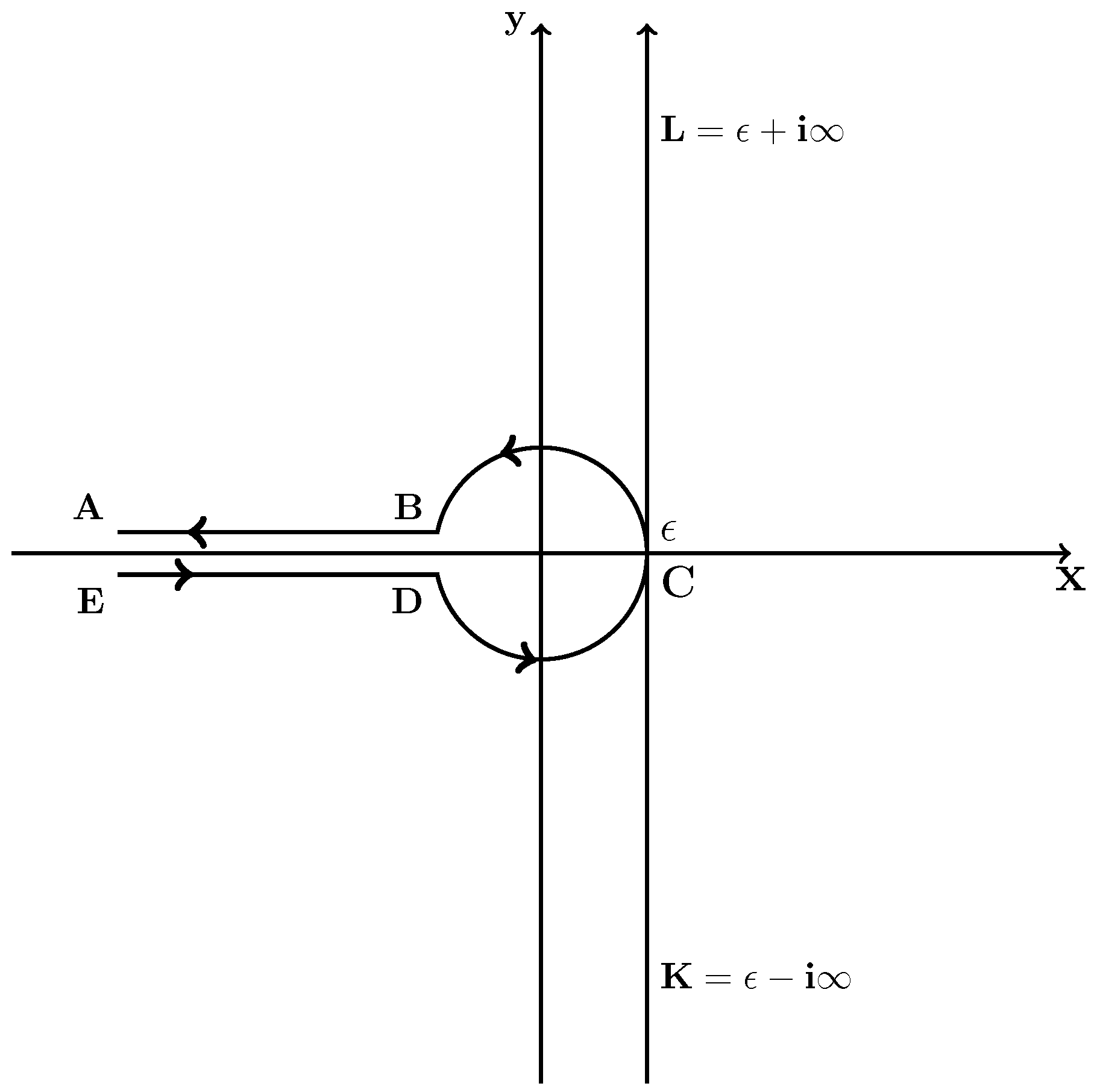
Theorem 4

(Complex GH Series Representation). Suppose that all indices $a_i$ and $b_i$ are real. Then for real z and $B>-1$

$$\begin{array}{c}\left[\begin{array}{ccc}\begin{array}{c}{a}_1,\dots ,a_p\\ B,b_1,\dots ,b_q\end{array}& \begin{array}{c}\dots \\ \dots \end{array}& \begin{array}{c}z\\ \end{array}\end{array}\right]=\frac{{(-1)}^{-B}\Gamma \left(B\right)}{2\pi i}{\int }_{H{a}^{+}}\frac{e^{-\tau }}{{\tau }^B}\left[\begin{array}{ccc}\begin{array}{c}{a}_1,\dots ,a_p\\ b_1,\dots ,b_q\end{array}& \begin{array}{c}\dots \\ \dots \end{array}& \begin{array}{c}-\frac{z}{\tau }\\ \end{array}\end{array}\right]d\tau =\\ \hfill \frac{\Gamma \left(B\right)}{2\pi i}{\int }_{H{a}^{-}}\frac{e^{\tau }}{{\tau }^B}\left[\begin{array}{ccc}\begin{array}{c}{a}_1,\dots ,a_p\\ b_1,\dots ,b_q\end{array}& \begin{array}{c}\dots \\ \dots \end{array}& \begin{array}{c}\frac{z}{\tau }\\ \end{array}\end{array}\right]d\tau \end{array}$$

where Hankel path $H{a}^{+}$ starts at infinity on the real axis, encircling 0 in a positive sense, and returns to infinity along the real axis, respecting the cut along the positive real axis, while $H{a}^{-}$ is its reflection.

Proof. 

From the Heine’s formula for the reciprocal Gamma function representation

$$\frac{1}{\Gamma \left(z\right)}=\frac{{(-1)}^{-z}}{2\pi i}{\int }_{H{a}^{+}}\frac{e^{-\tau }}{{\tau }^z}d\tau =\frac{1}{2\pi i}{\int }_{H{a}^{-}}\frac{e^{\tau }}{{\tau }^z}d\tau$$

It follows that

$$\sum _{k=0}^{\infty }\frac{1}{\Gamma (k+b)}{c}_k{(-z)}^k=\frac{{(-1)}^{-b}}{2\pi i}\sum _{k=0}^{\infty }{\int }_{H{a}^{+}}\frac{e^{-\tau }}{{\tau }^{k+b}}{c}_k{z}^{k}d\tau =\frac{{(-1)}^{-b}}{2\pi i}{\int }_{H{a}^{+}}\frac{e^{-\tau }}{{\tau }^b}\sum _{k=0}^{\infty }{c}_k{\left(\frac{z}{\tau }\right)}^k$$

Therefore,

$$\left[\begin{array}{cc}\begin{array}{c}{a}_1,\dots ,a_p\\ b,b_1,\dots ,b_q\end{array}& \begin{array}{c}z\\ \end{array}\end{array}\right]=\frac{{(-1)}^{-b}\Gamma \left(b\right)}{2\pi i}{\int }_{H{a}^{+}}\frac{e^{-\tau }}{{\tau }^b}\left[\begin{array}{cc}\begin{array}{c}{a}_1,\dots ,a_p\\ b_1,\dots ,b_q\end{array}& \begin{array}{c}\frac{z}{\tau }\\ \end{array}\end{array}\right]d\tau$$

and

$$\left[\begin{array}{ccc}\begin{array}{c}{a}_1,\dots ,a_p\\ b,b_1,\dots ,b_q\end{array}& \begin{array}{c}\dots \\ \dots \end{array}& \begin{array}{c}z\\ \end{array}\end{array}\right]=\frac{{(-1)}^{-b}\Gamma \left(b\right)}{2\pi i}{\int }_{H{a}^{+}}\frac{e^{-\tau }}{{\tau }^b}\left[\begin{array}{ccc}\begin{array}{c}{a}_1,\dots ,a_p\\ b_1,\dots ,b_q\end{array}& \begin{array}{c}\dots \\ \dots \end{array}& \begin{array}{c}-\frac{z}{\tau }\\ \end{array}\end{array}\right]d\tau$$

by extension.  □

Corollary 4.

For $B>-1$ the following representation holds

$$\begin{array}{c}\left[\begin{array}{ccc}\begin{array}{c}{a}_1,\dots ,a_p\\ b_1,\dots ,b_q\end{array}& \begin{array}{c}\dots \\ (B,b)\end{array}& \begin{array}{c}z\\ \end{array}\end{array}\right]=\frac{{(-1)}^{-B}\Gamma \left(B\right)}{2\pi i}{\int }_{H{a}^{+}}\frac{e^{-\tau }}{{\tau }^B}\left[\begin{array}{ccc}\begin{array}{c}{a}_1,\dots ,a_p\\ b_1,\dots ,b_q\end{array}& \begin{array}{c}\dots \\ \dots \end{array}& \begin{array}{c}\frac{z}{{(-\tau )}^b}\\ \end{array}\end{array}\right]d\tau =\\ \hfill \frac{\Gamma \left(B\right)}{2\pi i}{\int }_{H{a}^{-}}\frac{e^{\tau }}{{\tau }^B}\left[\begin{array}{ccc}\begin{array}{c}{a}_1,\dots ,a_p\\ b_1,\dots ,b_q\end{array}& \begin{array}{c}\dots \\ \dots \end{array}& \begin{array}{c}\frac{z}{{\tau }^b}\\ \end{array}\end{array}\right]d\tau \end{array}$$

Remark 2.

This theorem can be interpreted as the inverse Laplace transform of a simpler Fox-Wright function. Moreover, the complex integral can be converted to a real integral for suitable functions [11].

Theorem 5

(Real GH Series Representation). Suppose that all indices $a_i$ and $b_i$ are real. Then for some real $A>0$ and $a>0$ and $z<1$

$$\left[\begin{array}{ccc}\begin{array}{c}{a}_1,\dots ,a_p\\ b_1,\dots ,b_q\end{array}& \begin{array}{c}(A,a)\\ \dots \end{array}& \begin{array}{c}z\\ \end{array}\end{array}\right]=\frac{1}{\Gamma \left(A\right)}{\int }_0^{\infty }{e}^{-\tau }{\tau }^{A-1}\left[\begin{array}{ccc}\begin{array}{c}{a}_1,\dots ,a_p\\ b_1,\dots ,b_q\end{array}& \begin{array}{c}\dots \\ \dots \end{array}& \begin{array}{c}z{\tau }^a\\ \end{array}\end{array}\right]d\tau$$

Proof. 

From the Gamma function representation

$$\Gamma \left(z\right)={\int }_0^{\infty }{e}^{-\tau }{\tau }^{z-1}d\tau ,z>0$$

it follows that

$$\sum _{k=0}^{\infty }\Gamma (ak+A)c_k{z}^k=\sum _{k=0}^{\infty }{\int }_0^{\infty }{e}^{-\tau }{\tau }^{ak+A-1}{c}_k{z}^{k}d\tau ={\int }_0^{\infty }{e}^{-\tau }{\tau }^{A-1}\sum _{k=0}^{\infty }{c}_k{\left(z{\tau }^a\right)}^k$$

Therefore,

$$\left[\begin{array}{ccc}\begin{array}{c}{a}_1,\dots ,a_p\\ b_1,\dots ,b_q\end{array}& \begin{array}{c}(A,a)\\ \dots \end{array}& \begin{array}{c}z\\ \end{array}\end{array}\right]=\frac{1}{\Gamma \left(A\right)}{\int }_0^{\infty }{e}^{-\tau }{\tau }^{A-1}\left[\begin{array}{ccc}\begin{array}{c}{a}_1,\dots ,a_p\\ b_1,\dots ,b_q\end{array}& \begin{array}{c}\dots \\ \dots \end{array}& \begin{array}{c}z{\tau }^a\\ \end{array}\end{array}\right]d\tau$$

provided that all parameters are real.

Corollary 5.

$$\left[\begin{array}{ccc}\begin{array}{c}A,a_1,\dots ,a_p\\ b_1,\dots ,b_q\end{array}& \begin{array}{c}\dots \\ \dots \end{array}& \begin{array}{c}z\\ \end{array}\end{array}\right]=\frac{1}{\Gamma \left(A\right)}{\int }_0^{\infty }{e}^{-\tau }{\tau }^{A-1}\left[\begin{array}{ccc}\begin{array}{c}{a}_1,\dots ,a_p\\ b_1,\dots ,b_q\end{array}& \begin{array}{c}\dots \\ \dots \end{array}& \begin{array}{c}z\tau \\ \end{array}\end{array}\right]d\tau$$

Remark 3.

The last Theorem can be interpreted as the Laplace transform of a simpler Fox-Wright function. Pogany et al. give essentially the same result as Corrollary 5 as Equation (7) in page 128 [12].

In summary, the section shows that a $(p,q)$ GHG series can be reduced to a $p+q$ multiple integrals of the Euler type.

5. Applications

5.1. Mittag-Leffler Functions

The 2 parameter Mittag-Leffler function [13,14] under the present convention will be denoted as

$$E_{a,b}\left(z\right):=\sum _{k=0}^{\infty }\frac{z^k}{\Gamma (ak+b)}=\frac{1}{\Gamma \left(b\right)}\left[\begin{array}{ccc}\begin{array}{c}1\\ -\end{array}& \begin{array}{c}-\\ (b,a)\end{array}& \begin{array}{c}z\\ \end{array}\end{array}\right]$$

This immediately gives the complex integral representation according to Corollary 4

$$E_{a,b}\left(z\right)=\frac{1}{2\pi i}{\int }_{H{a}^{-}}\frac{e^{\tau }}{{\tau }^b}\left[\begin{array}{cc}\begin{array}{c}1\\ -\end{array}& \begin{array}{c}\frac{z}{{\tau }^a}\\ \end{array}\end{array}\right]d\tau =\frac{1}{2\pi i}{\int }_{H{a}^{-}}\frac{e^{\tau }}{{\tau }^b}\frac{d\tau }{1-\frac{z}{{\tau }^a}}=\frac{1}{2\pi i}{\int }_{H{a}^{-}}\frac{{\tau }^{a-b}{e}^{\tau }}{{\tau }^a-z}d\tau$$

However, in this case the contour encloses the curve $|1-z/{\tau }^a|=1$.

Another example is the 3-parameter Mittag-Leffler function generalization, that is the Prabhakar function [15] defined as

$$E_{a,b}^{\gamma }\left(z\right):=\sum _{k=0}^{\infty }\frac{\Gamma (k+\gamma )z^k}{\Gamma \left(\gamma \right)\Gamma (ak+b)k!}=\frac{1}{\Gamma \left(b\right)}\left[\begin{array}{ccc}\begin{array}{c}\gamma \\ -\end{array}& \begin{array}{c}-\\ (b,a)\end{array}& \begin{array}{c}z\\ \end{array}\end{array}\right]$$

In this case

$$E_{a,b}^{\gamma }\left(z\right)=\frac{1}{\Gamma \left(\gamma \right)}{\int }_0^{\infty }{e}^{-\tau }{\tau }^{\gamma -1}W\left(\left.a,b\right|z\tau \right)d\tau$$

which leads to an integral involving the Wright function.

An interesting special case is the function $E_{a,1}^{\gamma }\left(z\right)$ which is a confluent Kummer (${}_1{F}_1$) hypergeometric function. In this case for $a>\gamma$

$$E_{a,1}^{\gamma }\left(z\right)=\left[\begin{array}{cc}\begin{array}{c}\gamma \\ a\end{array}& \begin{array}{c}z\\ \end{array}\end{array}\right]=\frac{1}{\mathcal{B}(a,a-\gamma )}{\int }_0^1{\tau }^{\gamma -1}{(1-\tau )}^{a-\gamma -1}{e}^{z\tau }d\tau$$

as expected.

5.2. The Kummer-Wright Function

In particular, the following representation can be stated for the basic GH function (the Kummer-Wright function)

$$\begin{array}{c}\left[\begin{array}{ccc}\begin{array}{c}-\\ -\end{array}& \begin{array}{c}(A,a)\\ (B,b)\end{array}& \begin{array}{c}z\\ \end{array}\end{array}\right]=\\ \frac{1}{\mathcal{B}(A,B-A)}{\int }_0^1{\tau }^{A-1}{(1-\tau )}^{B-A-1}\left[\begin{array}{ccc}\begin{array}{c}-\\ -\end{array}& \begin{array}{c}-\\ (B-A,b-a)\end{array}& \begin{array}{c}z{\tau }^a{(1-\tau )}^{(b-a)}\\ \end{array}\end{array}\right]d\tau =\\ \hfill \frac{\Gamma \left(A\right)}{\Gamma \left(B\right)}{\int }_0^1{\tau }^{A-1}{(1-\tau )}^{B-A-1}W\left(\left.b-a,B-A\right|z{\tau }^a{(1-\tau )}^{(b-a)}\right)d\tau \end{array}$$

And also

$$\begin{array}{c}\left[\begin{array}{ccc}\begin{array}{c}-\\ -\end{array}& \begin{array}{c}(A,a)\\ (B,b)\end{array}& \begin{array}{c}z\\ \end{array}\end{array}\right]=\\ \frac{1}{\mathcal{B}(A,B-A)}{\int }_0^{\infty }\frac{u^{B-A-1}}{{\left(u+1\right)}^B}\left[\begin{array}{ccc}\begin{array}{c}-\\ -\end{array}& \begin{array}{c}-\\ (B-A,b-a)\end{array}& \begin{array}{c}\frac{z{u}^{b-a}}{{\left(u+1\right)}^a}\\ \end{array}\end{array}\right]du=\\ \hfill \frac{\Gamma \left(A\right)}{\Gamma \left(B\right)}{\int }_0^{\infty }\frac{u^{B-A-1}}{{\left(u+1\right)}^B}W\left(\left.b-a,B-A\right|\frac{z{u}^{b-a}}{{\left(u+1\right)}^a}\right)du\end{array}$$

This Wright function in turn can be represented as (see Equation (A4)):

$$W\left(\left.b-a,B-A\right|z\right)=\frac{1}{2\pi i}{\int }_{H{a}^{-}}{e}^{\tau }\frac{e^{z/{\tau }^{b-a}}}{{\tau }^{B-A}}d\tau$$

For the homogeneous case then

$$W\left(\left.0,B-A\right|z\right)=\frac{e^z}{\Gamma (B-A)}$$

according to the representation of the reciprocal Gamma function. Therefore, according to the Homogeneous Reduction Corollary:

$$\left[\begin{array}{ccc}\begin{array}{c}-\\ -\end{array}& \begin{array}{c}(A,a)\\ (B,a)\end{array}& \begin{array}{c}z\\ \end{array}\end{array}\right]=\frac{1}{\mathcal{B}(A,B-A)}{\int }_0^1{\tau }^{A-1}{(1-\tau )}^{B-A-1}{e}^{z{\tau }^a}d\tau$$

which is a generalization of the Kummer function.

5.3. Generalized Fractional Erdélyi-Kober Operations

The theory of GHG series has an interesting relationship with the generalized fractional calculus. The right Erdélyi-Kober (E-K) fractional integrals are defined as [10]:

$$I_{\beta }^{\gamma ,\delta }f\left(z\right):=\frac{1}{\Gamma \left(\delta \right)}{\int }_0^1{\tau }^{\gamma }{(1-\tau )}^{\delta -1}f\left({\tau }^{1/\beta }z\right)d\tau$$

while another equivalent form is [16] [Ch. 18]:

$$I_{\beta }^{\gamma ,\delta }f\left(z\right)=\frac{\beta z^{-\beta (\gamma +\delta )}}{\Gamma \left(\delta \right)}{\int }_0^z{(z^{\beta }-u^{\beta })}^{\delta -1}{u}^{\beta (\gamma +1)-1}f\left(u\right)du$$

The two forms are related by the change of variables $u=z{\tau }^{1/\beta }$. Therefore, from the preceding presentation it follows that

$$I_{1/\beta }^{\gamma ,\delta }\left[\begin{array}{ccc}\begin{array}{c}\dots \\ \dots \end{array}& \begin{array}{c}\dots \\ \dots \end{array}& \begin{array}{c}z\\ \end{array}\end{array}\right]=\frac{\Gamma (\gamma +1)}{\Gamma (\gamma +\delta +1)}\left[\begin{array}{ccc}\begin{array}{c}\dots \\ \dots \end{array}& \begin{array}{c}\dots ,(\gamma +1,\beta )\\ \dots ,(\gamma +\delta +1,\beta )\end{array}& \begin{array}{c}z\\ \end{array}\end{array}\right]$$

(3)

This corresponds to the findings of Kiryakova [17].

The E-K operator reduces to the Riemann-Liouville fractional integral for $\beta =1$ and $\gamma =0$ as

$$I_{R-L}^{\delta }f\left(z\right)=z^{\delta }{I}_1^{0,\delta }f\left(z\right)=\frac{z^{\delta }}{\Gamma \left(\delta \right)}{\int }_0^1{(1-\tau )}^{\delta -1}f\left(\tau z\right)d\tau$$

Conversely,

$$I_{R-L}^{\delta }{z}^{\gamma }f\left(z\right)=z^{\gamma +\delta }{I}_1^{\gamma ,\delta }f\left(z\right)$$

It is interesting to note further that the EK operators map the functions of the Dimovski space $D_{\alpha }$ into one another [18]:

$$I_{\beta }^{\gamma ,\delta }:{\mathbb{D}}^{\alpha }\mapsto {\mathbb{D}}^{\alpha },\alpha >-\beta (\gamma +1)$$

where the function space is given by the following:

Definition 1

(Dimovski Space [19]). The space of functions ${\mathbb{D}}^{\alpha }$ consists of all functions $f\left(x\right),x>0$, that can be represented in the form $f\left(x\right)=x^p{f}_1\left(x\right)$ with $p>\alpha$ and $f_1\in \mathbb{C}\left([0,\infty )\right)$.

The corresponding generalized Erdélyi-Kober fractional derivative is defined by a composition product as

$$D_{\beta }^{\gamma ,\delta }f\left(z\right)=\prod _{j=1}^{[\delta ]+1}\circ \left(\frac{z}{\beta }{\partial }_z+\gamma +j\right)I_{\beta }^{\gamma +\delta ,1-<\delta >}f\left(z\right)$$

where $<\delta >$ is the fractional part and $[\delta ]$ is the integral part of the number.

For $\beta =1$ the E-K fractional derivative operator reduces to the Riemann-Liouville fractional derivative of order $\delta$ as

$$D_{R-L}^{\delta }f\left(z\right)=D_1^{0,\delta }{z}^{-\delta }f\left(z\right)$$

The E-K fractional derivative operator is the left-inverse of E-K integral for suitable functions from ${\mathbb{D}}^{\alpha }$:

$$D_{\beta }^{\gamma ,\delta }{I}_{\beta }^{\gamma ,\delta }f\left(z\right)=f\left(z\right)$$

Therefore,

$$\left[\begin{array}{ccc}\begin{array}{c}\dots \\ \dots \end{array}& \begin{array}{c}\dots \\ \dots \end{array}& \begin{array}{c}z\\ \end{array}\end{array}\right]=\frac{\Gamma (\gamma +1)}{\Gamma (\gamma +\delta +1)}{D}_{1/\beta }^{\gamma ,\delta }\left[\begin{array}{ccc}\begin{array}{c}\dots \\ \dots \end{array}& \begin{array}{c}\dots ,(\gamma +1,\beta )\\ \dots ,(\gamma +\delta +1,\beta )\end{array}& \begin{array}{c}z\\ \end{array}\end{array}\right]$$

and

$$\left[\begin{array}{ccc}\begin{array}{c}\dots \\ \dots \end{array}& \begin{array}{c}\dots \\ \dots \end{array}& \begin{array}{c}z\\ \end{array}\end{array}\right]=\frac{\Gamma \left(\gamma \right)}{\Gamma \left(\delta \right)}{D}_{1/\beta }^{\gamma -1,\delta -\gamma }\left[\begin{array}{ccc}\begin{array}{c}\dots \\ \dots \end{array}& \begin{array}{c}\dots ,(\gamma ,\beta )\\ \dots ,(\delta ,\beta )\end{array}& \begin{array}{c}z\\ \end{array}\end{array}\right]$$

(4)

The last equation can be used for index reduction.

6. Discussion

These results demonstrate that the homogeneous class of GHG series are closed with respect to the (generalized) fractional calculus operations. One can, therefore, expect that the solutions of fractional differential equations could be expressed in terms of Fox-Wright functions. Therefore, the Fox-Wright functions are the most general functions of the mathematical physics.

Furthermore, the results demonstrate a strong link between the special function theory and the theory of the Euler Beta and Gamma functions. It appears that the E-K operators can be thought of Euler’s Beta integrals in disguise. Moreover, the Gamma integral representations can be interpreted as Laplace or Inverse Laplace transforms.

Finally, the main consequence of so-presented results is that all GHG functions of the Fox-Wright type can be represented as multiple (complex) integrals of three primitive special functions of orders $(1,0)$, $(0,1)$ and $(1,1)$ respectively. This corroborates the findings of Kiryakova [9,10,17]. These multiple integrals can be denoted as generalized fractional differ-integrals; however, this line of representation is superfluous to the necessities of the numerical and physical modeling.

References

1. Kilbas, A.; Saigo, M.; Truijllo, J.J. On the generalized wright function. Fract. Calc. Appl. Anal. 2002, 5, 437–460. [Google Scholar]
2. Haubold, H.J.; Mathai, A.M.; Saxena, R.K. Mittag-Leffler functions and their applications. J. Appl. Math. 2011, 2011, 298628. [Google Scholar] [CrossRef]
3. Rogosin, S. The Role of the Mittag-Leffler Function in Fractional Modeling. Mathematics 2015, 3, 368–381. [Google Scholar] [CrossRef]
4. Gorenflo, R.; Luchko, Y.; Mainardi, F. Wright functions as scale-invariant solutions of the diffusion-wave equation. J. Comput. Appl. Math. 2000, 118, 175–191. [Google Scholar] [CrossRef]
5. Mainardi, F.; Mura, A.; Pagnini, G. The M-Wright function in time-fractional diffusion processes: A tutorial survey. Int. J. Differ. Equ. 2010, 2010, 1–29. [Google Scholar] [CrossRef]
6. Oldham, K.; Spanier, J. The Fractional Calculus: Theory and Applications of Differentiation and Integration to Arbitrary Order; Academic Press: New York, NY, USA, 1974. [Google Scholar]
7. Wright, E.M. The asymptotic expansion of the generalized hypergeometric function. J. Lond. Math. Soc. 1935, 1, 286–293. [Google Scholar] [CrossRef]
8. Wright, E.M. The asymptotic expansion of integral functions defined by Taylor series. Philos. Trans. R. Soc. A Math. Phys. Eng. Sci. 1940, 238, 423–451. [Google Scholar] [CrossRef]
9. Kiryakova, V. All the special functions are fractional differintegrals of elementary functions. J. Phys. A Math. Gen. 1997, 30, 5085–5103. [Google Scholar] [CrossRef]
10. Kiryakova, V. The special functions of fractional calculus as generalized fractional calculus operators of some basic functions. Comput. Math. Appl. 2010, 59, 1128–1141. [Google Scholar] [CrossRef]
11. Prodanov, D. Regularized Integral Representations of the Reciprocal Gamma Function. Fractal Fract. 2019, 3, 1. [Google Scholar] [CrossRef]
12. Pogány, T.K.; Srivastava, H.M. Some Mathieu-type Series Associated with the Fox-Wright Function. Comput. Math. Appl. 2009, 57, 127–140. [Google Scholar] [CrossRef]
13. Mittag-Leffler, G.M. Sur la nouvelle fonction Ea(x). C. R. Acad. Sci. Paris 1903, 137, 554–558. [Google Scholar]
14. Wiman, A. Über den Fundamentalsatz in der Teorie der Funktionen Ea(x). Acta Math. 1905, 29, 191–201. [Google Scholar] [CrossRef]
15. Prabhakar, T.R. A singular equation with a generalized Mittag-Leffler function in the kernel. Yokohama Math. J. 1971, 19, 7–15. [Google Scholar]
16. Samko, S.; Kilbas, A.; Marichev, O. Fractional Integrals and Derivatives: Theory and Applications; Gordon and Breach: Yverdon, Switzerland, 1993. [Google Scholar]
17. Kiryakova, V. Fractional calculus operators of special functions? The result is well predictable! Chaos Solitons Fractals 2017, 102, 2–15. [Google Scholar] [CrossRef]
18. Luchko, Y. Algorithms for evaluation of the Wright function for the real arguments’ values. Fract. Calc. Appl. Anal. 2008, 11, 57–75. [Google Scholar]
19. Dimovski, I. Operational calculus for a class of differential operators. C. R. Acad. Bulg. Sci. 1966, 19, 1111–1114. [Google Scholar]
20. Mainardi, F.; Luchko, Y.; Pagnini, G. The fundamental solution of the space-time fractional diffusion equation. Fract. Calc. Appl. Anal. 2001, 4, 153–192. [Google Scholar]