Predicting Cell Cleavage Timings from Time-Lapse Videos of Human Embryos

Abstract

Assisted reproductive technology is used for treating infertility, and its success relies on the quality and viability of embryos chosen for uterine transfer. Currently, embryologists manually assess embryo development, including the time duration between the cell cleavages. This paper introduces a machine learning methodology for automating the computations for the start of cell cleavage stages, in hours post insemination, in time-lapse videos. The methodology detects embryo cells in video frames and predicts the frame with the onset of the cell cleavage stage. Next, the methodology reads hours post insemination from the frame using optical character recognition. Unlike traditional embryo cell detection techniques, our suggested approach eliminates the need for extra image processing tasks such as locating embryos or removing extracellular material (fragmentation). The methodology accurately predicts cell cleavage stages up to five cells. The methodology was also able to detect the morphological structures of later cell cleavage stages, such as morula and blastocyst. It takes about one minute for the methodology to annotate the times of all the cell cleavages in a time-lapse video.

1. Introduction

Assisted reproductive technology (ART) is a treatment for individuals or couples, who are unable to conceive a child. ART techniques such as in vitro fertilization (IVF) or intracytoplasmic sperm injection (ICSI) involve fertilization of the egg outside the female body. Several oocytes (unfertilized eggs) are surgically removed from the ovary of the woman and fertilized with sperm in a laboratory, resulting in embryos. The embryos are cultured in an incubator with optimal conditions for a maximum of five days. The cultured embryos can be transferred into the uterus, cryopreserved for subsequent transfers, or discarded. Typically, the embryo with the highest quality is transferred back to the woman’s uterus. The process of estimating the quality of each embryo and ranking the available embryos within a cohort is called embryo evaluation [1,2]. The embryo evaluation is carried out manually by embryologists. 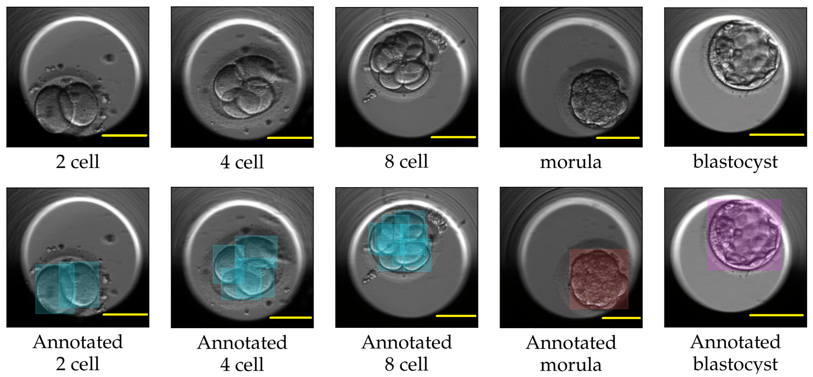The embryologists rank each embryo based on various criteria proven to be correlated with successful implantation or childbirth [3,4]. One such criterion involves analyzing the dynamics of the cell cleavage stages, also referred to as the morphokinetic parameters related to embryo development. A cell cleavage stage is characterized by the number of embryonic cells and their subsequent cell division. An example of a human embryo monitored for development from the two-cell stage, three-cell stage, and four-cell stage to later stages such as the morula and blastocyst stage are shown in Figure 1. The morula and blastocyst stages have a distinct morphology as compared to the early cell cleavage stages of embryo development. The morula stage is a compacted structure made of small-sized cells followed by a blastocyst, which is composed of hundreds of cells characterized into distinct features.

Evaluating the morphological development of cell cleavages is a relevant step in selecting embryos with high quality and viability [5,6]. The embryologists assess morphokinetic parameters such as changes in the cell morphology and the transitions during cell division to identify embryos with a higher potential to implant [7,8]. The information on cell cleavage duration is important for embryo evaluation [9]. The time between subsequent embryo cell divisions, including both absolute and relative timings is relevant [10]. Research has shown that in the embryos with a higher potential to implant, the cleavage from two cells to eight cells occurred comparatively earlier [11] than in embryos that were unable to implant. A study concluded that evaluating the exact timing of embryo division in the early cleavage stages has a high potential to predict embryo quality [12]. Another study revealed that the time taken to divide to five cells and the time between the division from three cells to four cells can effectively determine the embryo quality [13]. Indeed, the evaluation of the exact timing of early events in embryo development is a promising tool for predicting embryo quality [12], and progression from one cleavage to the next cleavage represents a noninvasive marker of embryo development potential [14,15]. Therefore, detecting the cell cleavage stages and the timings of successive cleavage during the preimplantation phase can provide valuable insights into embryo viability.

Usually, embryologists manually examine the cell cleavage stages and the length of the cleavage cycles [16], and it should take less than 2 min to annotate a single embryo, but often a single patient has multiple embryos (5–10 embryos), so it can take up to 20 min [17]. However, this task can be tedious and prone to subjectivity. The process can be automated using artificial intelligence (AI) or, specifically, object detection algorithms and optical character recognition (OCR). In fact, in recent times, several AI algorithms have been applied to automate embryo evaluation [2,18,19,20]. The application of object detection algorithms for medical image processing is common [21]. The medical domain images usually have the object of interest as a small surface area and blurred boundary [22]. 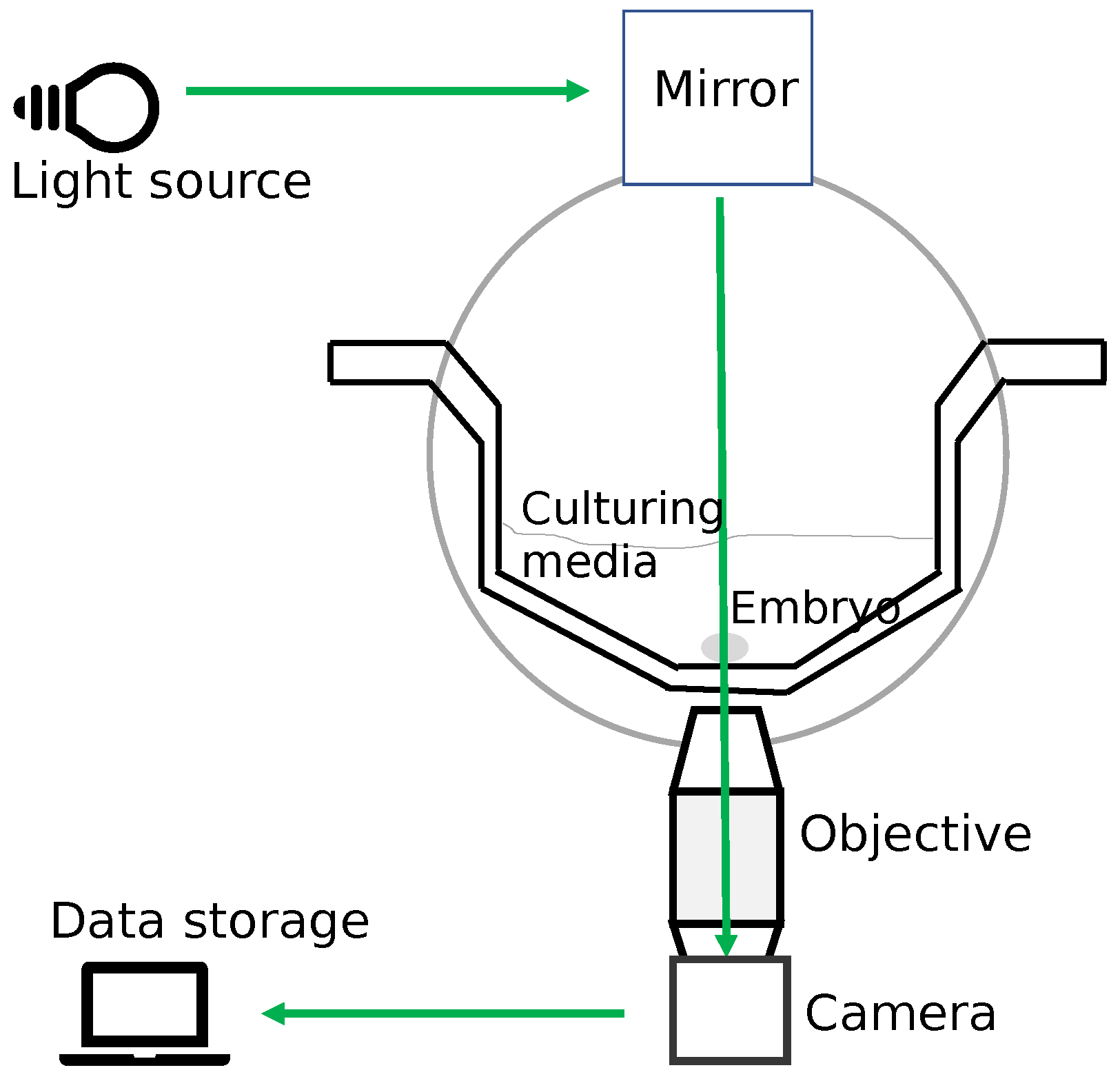However, the algorithms effectively detect the object in both images [23] and video stream [24]. A similar characteristic was observed for embryo cells with the application of time-lapse imaging. The time-lapse technology (TLT) enables the continuous monitoring of embryo development [25,26] and provides comprehensive information regarding the morphokinetics of embryo development including observations for events such as cell division or the transition between different cell cleavage stages [27]. With the application of an object detection algorithm, we can detect cells inside an embryo and determine the associated cell cleavage stage. The time-lapse imaging also captures the elapsed time since the start of fertilization. Depending upon the time-lapse system software, usually, the hours post insemination (hpi) is appended to each frame of video and can be read by the application of optical character recognition (OCR). Thus, using object detection and OCR we can automate the process of finding the start of an observed cell cleavage stage and recognizing the associated time in hpi (absolute or relative) for the stage. The automation will benefit embryologists in their daily tasks and can be used as a decision support system.

The software iDAScore from Vitrolife automatically estimates cell division events in time lapse. The feature is referred to as Guided Annotation [28]. The software requires a license and also the presence of Vitrolife EmbryoScope, EmbryoViewer software, which makes it cost intensive. Moreover, the quality of the TLT video is important for Guided Annotation’s efficient performance. For example, during the entire period, the embryo should be centered and in focus with entire embryo region being visible. There are alternative noninvasive approaches to count the number of cells and their location in time-lapse images of embryo development [29,30,31]. Their algorithms are based on computer vision and machine learning and predict only the cell count but no time annotations for the cell cleavage stages. Moreover, the algorithms require additional preprocessing steps such as image processing, detecting the embryo location, or extra filters to grasp the morphology progression along the temporal domain. This makes the approaches resource-demanding. Furthermore, the approaches only detect the early stages of embryo development and do not apply to later stages such as morula and blastocyst.

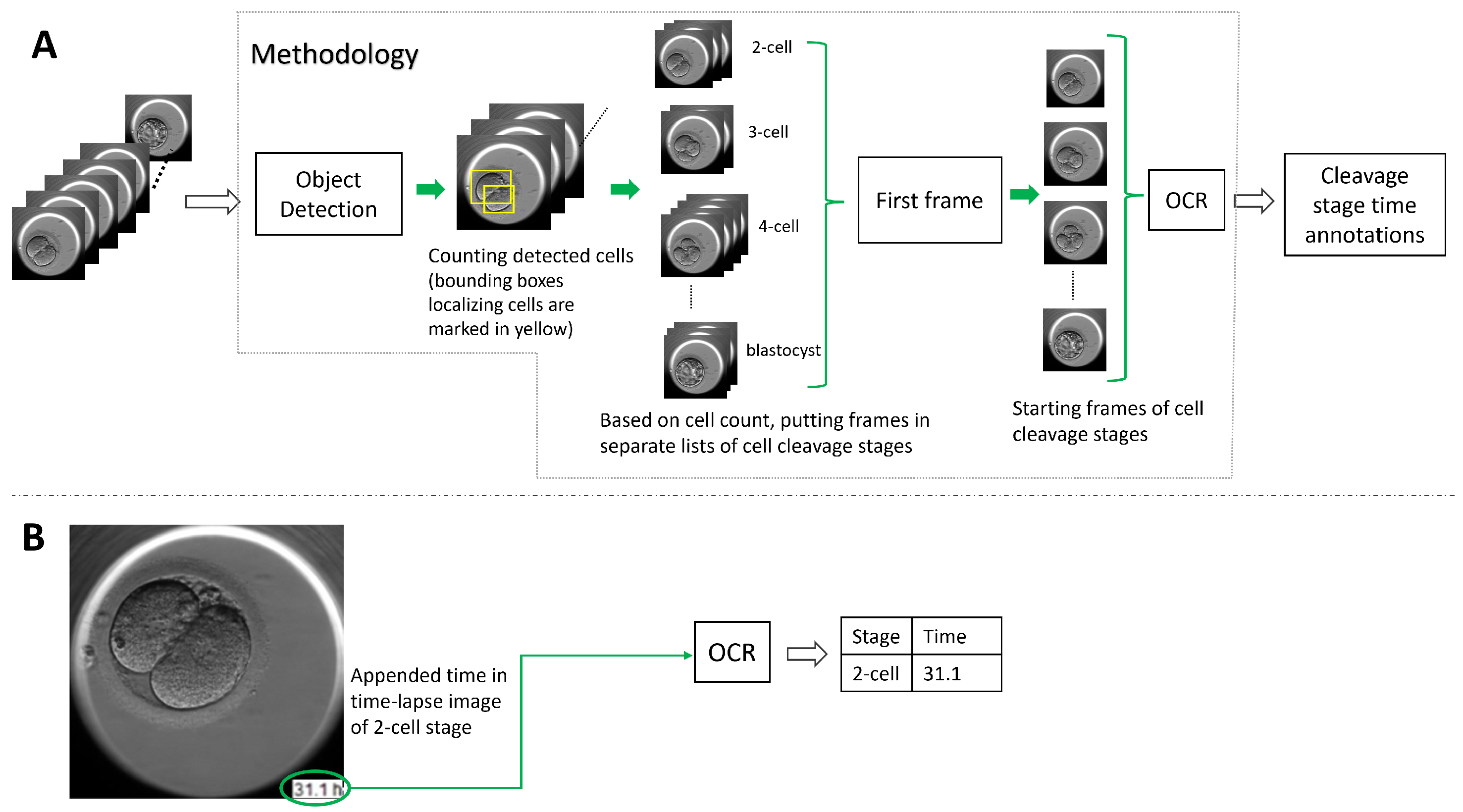
To address the lack of time annotation in previous research, in this article, we suggest a novel methodology for identifying the start and duration of cell cleavage stages in TLT videos. The methodology uses object detection algorithms to analyze each frame in the video and identify instances of cells, as well as the presence of the morula and blastocyst stages. The frames that belong to a cell cleavage stage are grouped together based on the number of cells or the presence of the morula and blastocyst. The first frame in each group is annotated as the start of the cleavage stage, and the hpi present on that frame is read using OCR. If the hpi value is missing, the methodology derives it using the video frame rate and time-lapse system configuration. We evaluated two object detection algorithms (YOLO v5 and DETR, explained in Section 3.1) and three OCR techniques (pytesseract, EasyOCR, and Keras-OCR, explained in Section 3.2) with our methodology. In Figure 2, we outline the methodology’s workflow.

The suggested methodology is capable of not only locating the cells but also predicting the start of all cell cleavage stages observed in a TLT video. Furthermore, we found that the presence of artifacts or fragmentation in the datasets did not affect the performance, since our methodology was able to differentiate them from the cells. The methodology operates directly on TLT video frames without any additional preprocessing steps or software license installation, making it both cost- and time-effective. For patients with the number of embryos in the range of 5–10, the methodology used, on average, around 3 min to compute the annotations of all the TLT videos. To best of our knowledge, besides iDAScore, there exists no other software tool that computes automated cell cleavage annotations. Thus, the combination of object detection with OCR in the field of ART and for the automated annotating of morphokinetics parameters is novel.

The main contributions in the article are as follows:

• We have developed a fully automated framework for tracking cell divisions and counting cells in embryos.
• Our methodology predicts and annotates the start time of cell cleavages without the need for any manual intervention by embryologists.
• Our methodology effectively detects the starting frame of cell cleavage stages from one cell to five cells, and achieved an F1-score of 0.63 and an accuracy of 0.69. For detecting the starting frames for stages with cell counts greater than five, our methodology was delayed by 30–32 frames on average, considering videos with a frame rate of eight frames per hour. The time annotations for the two-cell to five-cell stages were delayed by 2–3 hpi on average.
• Our methodology’s versatility allows it to accurately detect not only the number of cells in an embryo but also the distinct morphological structures of later cell cleavage stages, such as the morula and blastocyst.
• We examined the relation between the level of fragmentation within an embryo and the performance of our proposed methodology. Embryologists’ validation confirmed that our approach did not confuse cells with small-sized fragments.
• Our methodology computes start-time annotations (in hpi) for videos in real time, making it suitable for clinical applications. The shortest video was annotated in 26 s, while the longest video took approximately one minute.

The rest of the paper is organized as follows: Section 2 provides an overview of the existing methodologies automating the detection of the cell cleavage stages, and Section 3 provides an overview of the state-of-the-art object detection algorithms and OCR libraries. Section 3 also describes the principle theory behind time-lapse systems. Section 4 describes the data used for training and evaluation of the methodology, and Section 5 provides an overview and discusses various components of the methodology. Section 6 and Section 7 discuss the results and their limitations along with suggestions for future research. Finally, Section 8 concludes the paper and highlights the main findings.

2. Related Work

In this section, we review previous research work for detecting cell cleavage stages in TLT videos of human embryo development. In Section 2.1 we present some research studies employing different techniques to predict cell count and eventually the associated cell cleavage stage.

2.1. Predicting Cell Cleavage Stages

Various research studies have explored detecting embryo cells and predicting cell cleavage stages of human embryos in time-lapse images. A few methods have used a particle filter for tracking cell divisions [9] or developed conditional random field (CRF) framework for counting cells and predicting cell division [30,32]. Another approach used the Markov chain model to infer the most likely number and location of cells in a human embryo [33]. However, the application of these approaches is challenged by the exponentially growing search space. The search space is constituted with tracking multiple cell divisions. Thus, the approaches are limited to only detecting the early cell cleavage stages of embryo development. Moreover, these approaches relied on handcrafted feature sets and detailed annotations. Detailed annotations were also a prerequisite for an approach to detecting cells by predicting the density of cells instead of their precise location [34]. Since the annotations estimated the cells’ local density, the task of generating annotations alone was time-consuming and challenging. Deep-learning-based approaches have also been applied for detecting human embryo cell cleavage stages. In another study, AlexNet and VGG16 were used to classify the embryo cell cleavage stages after determining the rough location of the embryo using a Haar feature-based cascade classifier and marking the embryo boundary using the gradient vector for image pixels [17]. Another approach employed a convolutional neural network (CNN) to count cells and used CRF to include temporal information when predicting the cell cleavage stage [31]. The framework required preprocessing of the input images such as removing the petri dish, cropping the embryo, putting the cells into focus, and filtering to remove fragmentation.

However, these approaches are limited to detecting only early cell cleavage stages and often require preprocessing of images or detailed annotations. In contrast, our methodology directly uses state-of-the-art object detection algorithms to detect the cells, morula, and blastocyst stages in raw TLT video frames without any preprocessing requirements. This makes it suitable for real-time processing in clinical settings, and unlike proprietary software such as iDAScore, our methodology was developed using open-source libraries and is not dependent on any specific time-lapse system.

3. Background Theory

This section explain the concepts such as the state-of-the-art AI techniques and TLT. Section 3.1 focuses on the object detection algorithms used in our methodology for identifying cells, morula, and blastocyst in TLT videos. Section 3.2 discusses the optical character recognition (OCR) libraries used for computing time annotations in hpi, while Section 3.3 provides a brief overview of the TLT used for monitoring embryo development.

3.1. Object Detection Algorithms

Object detection in an image or a video is defined as proposing the region of interest to find what the region represents (classification) and where it is located (localization) and then creating bounding boxes for the detected objects [35,36]. These objects are instances of predefined classes. The knowledge about the location of an object will help in object tracking and gathering information about the object’s speed and evolution in shape, position, and structure. The rapid progress in deep learning has provided great momentum to object detection technology, and currently there exist several object detection algorithms such as YOLO (You Only Look Once), SSD (Single Shot Multibox detector), region proposals (R-CNN, Fast-RCNN, Faster RCNN, Cascade R-CNN), RetinaNet, and DEtection TRansformer (DETR) to name a few.

In ART, the embryo morphology is analyzed in real time; hence, a fast object detection technology is required. YOLO [37] is a much faster algorithm than its counterparts such as Region proposals [36]. The object detection algorithms such as YOLO, Mask R-CNN, Faster R-CNN, etc., perform auxiliary tasks such as non-maximum suppression (NMS) when detecting objects. DETR is different because it does not conduct auxiliary tasks and uses a set-based global loss for uniquely predicting object locations [38]. Thus, our methodology evaluated two object detection algorithms: YOLO and DETR to detect instances of cell, morula, and blastocyst.

YOLO v5 is a single-shot detector that processes the entire image at once, performing both detection and classification simultaneously. The image is divided into N grids of equal size, and for each grid, the algorithm predicts the probability of an object being present within the grid. These grids’ regions, called anchor boxes, are tunable parameters. During training, the anchor boxes inform the algorithm about the image regions it should process regularly for successful detection and classification in a single forward pass. YOLO v5 draws bounding boxes around objects, weighs them with an expected probability of locating the object against its class label, and uses the mean average precision (mAP) metric to quantify performance while predicting bounding boxes for different object classes. The mAP is the mean of the average precision (AP) for all the object classes and AP summarizes the precision-sensitivity curve for YOLO v5 when predicting the bounding box per object class into a single value. The single value provides an average of all the precision values. The algorithm can identify several bounding boxes for a single object. However, to choose the best box and remove the others, the non-maximum suppression (NMS) technique is applied. NMS starts by selecting the box (BC) with the highest confidence level and then calculates the intersection between the BC and the other candidate boxes. Next, the intersection is divided by the union between the BC and the other boxes to obtain the Intersection over Union (IoU) value, see Figure 3. If the IoU value exceeds a predetermined threshold, the other box is filtered out. The selection of the best bounding box and the filtering of other box candidates is shown in Figure 4.

DETR is a new approach to object detection that eliminates auxiliary heuristics such as NMS and trains end-to-end for object detection. It works by using a CNN to extract features from an image and a transformer to detect objects related to those features using the loss function called bipartite matching. The bipartite matching loss is shown in Figure 5.

The architecture of the DETR is divided into blocks: backbone, encoder, decoder, and prediction heads. The schematic diagram explaining the DETR architecture and the workflow of image processing is shown in Figure 6. An image is passed through the CNN to downscale the spatial extent and obtain feature maps. The flattened feature maps are passed as a token across the transformer consisting of the both encoder and decoder. Along with the feature maps, an additional element called positional encoding is also passed to the transformer. The positional encoding indicates to the transformer which position in the original image the elements in the feature maps correspond to, and this information is added to each layer of the transformer. The transformer has an attention mechanism and processes these tokens. In the encoder part, every token is mapped to a query, key, and value. The value vectors are summed, resulting in every token attending to other tokens and giving global attention. The value vectors are propagated through encoder layers and the generated representations to the decoder. The decoder also receives fixed N sized object queries. The N is fixed to 100 in the DETR architecture.

The queries initially start as random vectors and are responsible for locating objects within an image. The queries are trained to detect objects in a specific location in or part of an image. These queries act as positional encoding for the decoders, and the N output is passed on to a feed forward network (FFN) in parallel. The FFN then outputs a combination of bounding boxes and classes for each of the N detected objects. This output is placed in a set called the predicted set. The length of the predicted set is 100 and differs from that of the ground truth set. To account for this, the ground truth set is padded with ‘no object class’ and ‘empty bounding box coordinates’. Moreover, the predicted set may have several entries with ‘no object class’ and ‘empty bounding box coordinates’. The DETR uses bipartite matching loss to match entries in the predicted set to those in the ground truth set with the goal of finding the permutation of the predicted set closest to the ground truth set. The bipartite matching results in minimum loss, which is calculated using the IoU loss and the L1 loss (when bounding box coordinates are at an offset from their corresponding entry in the ground truth) combined with cross entropy loss (when a wrong class label is predicted). To perform an effective bipartite matching, the DETR uses the Hungarian optimization algorithm. According to the illustrated figure, the best permutation of the predicted set (in terms of color) incurring minimum loss will be pink to be on top, followed by yellow and then the ‘no object class’.

3.2. Optical Character Recognition Libraries

The output of the suggested methodology after processing a TLT video is the computation of time annotations in hpi for the start of the cell cleavage stages present in the video. One of the mechanisms used by the methodology to detect the hpi is the application of OCR to read out the appended hours on video frames (for reference, see Figure 2). OCR is the process of detecting text in an image and then converting the content into a machine-readable text format for analysis. We evaluated three open-source OCR libraries Python-tesseract (pytesseract) [40], EasyOCR [41], and Keras-OCR [42]. Pytesseract is a python wrapper for Google’s Tesseract-OCR engine. Tesseract is available under the Apache 2.0 license as an open-source engine. It can be used directly or with an API. To recognize a single character, the engine uses CNN, and for processing the sequence of characters, long short-term memory (LSTM) is employed. Pytesserect can read all types of images including jpeg, png, and gif to extract text from the images. To use pytesseract for OCR, our suggested methodology had to preprocess each frame. The frame was grayed out for regions other than the region containing the text. The library Keras-OCR is a packacked version of the Keras Convolutional Recurrent Neural Network (CRNN) [43] and the Character-Region Awareness For Text detection (CRAFT) [44] model and provides API for training text detection and OCR. Keras’s implementation of CRNN for text recognition utilizes the implementation of two models. The first one is based on the original CRNN model, and the second one includes a spatial transformer network layer to rectify the text [43]. The CRAFT text detector detects the text area by exploring each character region and affinity between the characters. The bounding box on the text is obtained by finding the minimum bounding rectangles after thresholding character regions with affinity scores [44].

3.3. Time-Lapse Technology

Embryo development is a dynamic event observed in both spatial and temporal domains. For culturing embryos outside the body, an optimal incubation environment in terms of temperature, pH, and oxygen levels is a basic requirement [45]. The TLT offers a stable optimal incubation environment for culturing embryos without removing them from the incubator. TLT also provides for the continuous monitoring of the dynamics of cell divisions for the embryo through multiple image acquisitions at frequent intervals [25]. The embryos are kept inside the TLT system culture media in a specially designed culturing dish. A TLT system has a standalone incubator primarily containing three components: (1) a light source to illuminate an embryo, (2) a digital inverted microscope to magnify the cells inside the embryo while the images are being captured, and (3) a digital camera to capture the images of an embryo (with the use of software, a TLT video can be made from the images depicting embryo development). Hence, TLT monitoring allows for the collection of a lot of information on the timings of the cell cleavages and other morphological changes [46]. Figure 7 shows a schematic design of a time-lapse incubator system.

In this study, we used a TLT system called Embryoscope^TM (Vitrolife). Embryoscope^TM is an incubator with an integrated time-lapse system, where the embryos are cultured individually in microwells and are moved one by one into the field of view of the inbuilt microscope at each instance of the image acquisitions captured by the inbuilt camera. In the Embryoscope^TM system, embryos are cultured in culture dishes called Embryoslides [46]. The specification of the system comes with a camera under a 635 nm LED light source passing through Hoffman’s contrast modulation optics. For each embryo placed inside the incubator, the system takes 8-bit images with a resolution of 500 × 500 pixels at several focal planes (number varying between 3 and 5) every 15 min. The images are processed to be displayed on a computer screen. Whenever the TLT system captures an image, it has the provision to encode the time (in hours) on the bottom right corner of the image. The time is calculated from the starting time of insemination for each oocyte individually. The captured images can then be connected to form a video that can rewind and fast forward for detailed analyses by embryologists. To analyze the progression of the embryo over time, the embryologist, for instance, can go through the video and identify the start of each observed cell cleavage stage. However, the annotating process requires manual intervention by the embryologists.

4. Data

The dataset consisted of TLT videos collected retrospectively by embryologists working at the Fertilitetssenteret. The Fertilitetssenteret is a fertility clinic in Oslo, Norway. The embryos were cultured inside an EmbryoscopeTM with similar time-lapse imaging specifications as described in Section 3.3. The dataset contained two types of videos: embryos that had been transferred to females and embryos that had been frozen or cryopreserved for later use. We used two separate categories to potentially improve the generalizability of the suggested methodology. For example, the frozen videos had a higher rate of fragmentation compared to the transferred videos. We used the transferred videos to train and validate the object detection algorithms, which we explain in Section 5.1. The dataset consisted of 250 videos and is referred to as the ‘TransferV’ dataset in the rest of the paper. Furthermore, the TransferV was further divided into a training set and an evaluation set consisting of 200 and 50 videos, respectively. The training set was used for training the object detection algorithms to locate instances of cells, morula, or blastocyst, while the evaluation set was used for evaluating the object detection algorithms and tuning the hyperparameters for efficient detection of the cell cleavage stages.

While TransferV was used to train and evaluate the object detection algorithms, the frozen embryo videos were used to evaluate the performance of our methodology to predict the start of the cell cleavage stages. The dataset consisted of 29 videos and is referred to as ‘FrozenV’ in the rest of the paper.

Table 1. Summary of the datasets used in this study. Each row provides the name of the dataset, the number and type of videos, whether the dataset was divided into subgroups, and a description of how the datasets were used.

Dataset Name	Videos	Type of TLT Videos	Use	Sub-Division
TransferV	250	Uterine Transfer	1. Train and evaluate object detection algorithms 2. Tune hyperparameters of the methodology	Training set Evaluation set
Training set	200	Uterine transfer	Train object detection algorithms to detect cells, morula, and blastocysts in TLT frames
Evaluation set	50	Uterine transfer	1. Evaluate trained object detection algorithms 2. Tune hyperparameters of the methodology
FrozenV	29	Cryopreserved	Evaluate the performance in predicting the start of cell cleavage stages

summarizes the different datasets that were used in this study.

For each video in the TransferV dataset, the embryologists at the Fertilitetssenteret reviewed all the video frames and manually annotated the start (hpi and frame number) of the observed cell cleavage stage. We used the annotations to extract the representative frame by marking the start of the cell cleavage stages in the videos. The training set consisted of frames only belonging to the two-cell, four-cell, five-cell, eight-cell, nine+-cell, morula, and blastocyst cleavage stages, while the evaluation set consisted of representative frames for all the cell cleavage stages from the one-cell to the blastocyst stage. The frames in training set were annotated with class labels as cells, morula, or blastocyst using the applications Labelbox [47] and Roboflow [48]. Figure 8 shows some labels created with LabelBox. We further applied augmentation techniques, such as horizontal and vertical flip and rotation between −30° amd 30°, to increase the number of class labels. In total, we created 3868 class labels, 3490 for cells, 188 for morula, and 190 for blastocysts. The accurateness of the created class labels using LabelBox and Roboflow were approved by the embryologists.

Three embryologists independently reviewed the FrozenV dataset videos frame by frame and annotated the start of the cell cleavage stages (time and frame number). These embryologists are referred to as E1, E2, and E3 in the rest of the paper. The annotations from all three embryologists were used to evaluate the methodology’s performance in predicting the start of cell cleavage stages. However, 0.5 percent of the manual annotations were incorrect. To rectify this, we replaced the incorrect annotations with the average value calculated from the annotations of the two other embryologists.

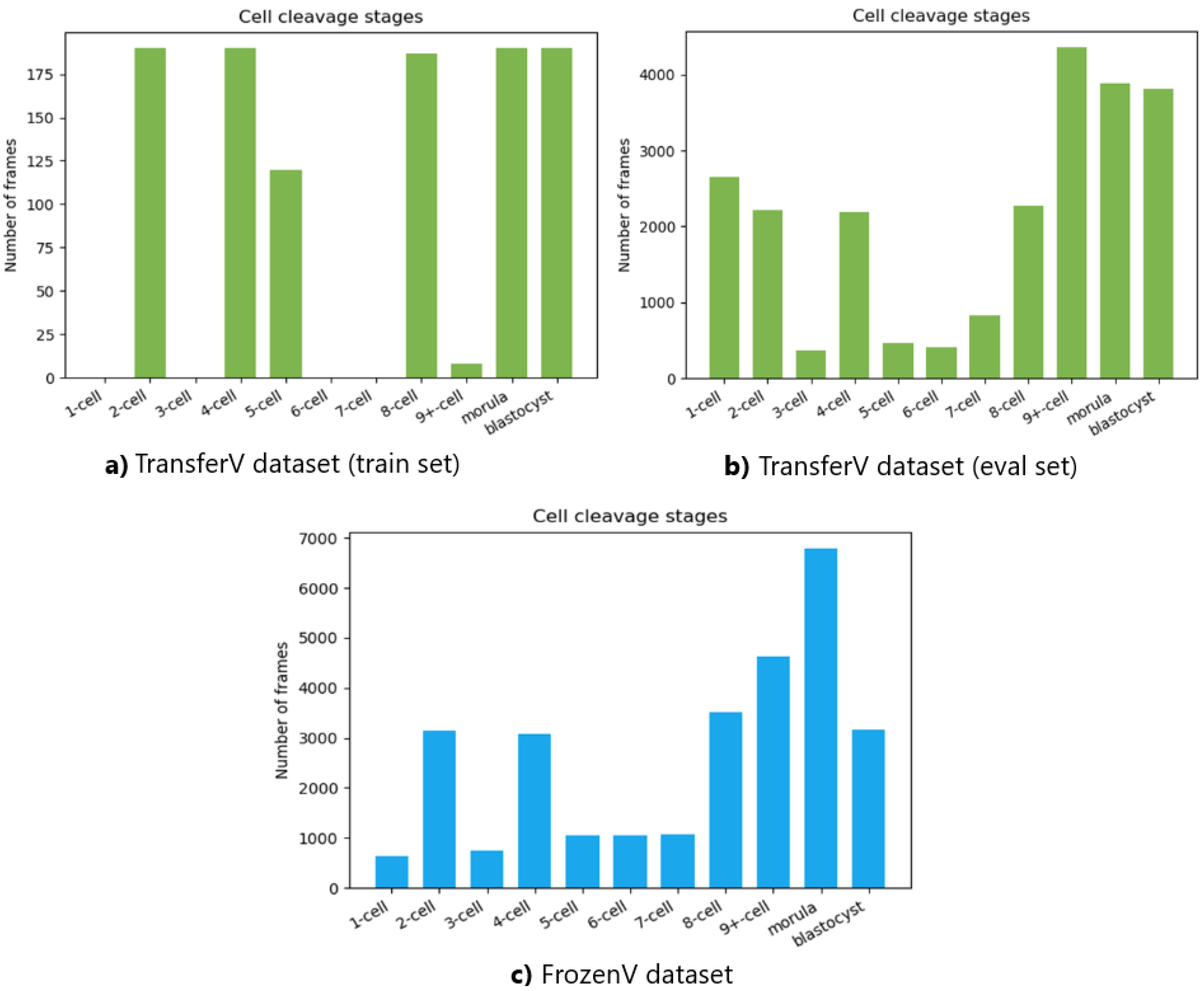
The number of frames in the videos for each cell cleavage stage in the TransferV and FrozenV datasets is shown in Figure 9. The cell cleavage stages are characterized by the presence of a specific number of cells, morula, or blastocyst. Thus, we also present the distribution of instances for cells, morula, and blastocysts for both datasets in

Table 2. The class objects (cells, morula, and blastocyst) count in datasets. The datasets are used in the training and evaluation of the methodology.

Dataset	Cell	Morula	Blastocyst
TransferV dataset	111,954	6975	3357
FrozenV dataset	87,073	3928	4064

.

As mentioned before, E1, E2, and E3 independently annotated the FrozenV dataset. Thus, we combined the three independent set of annotations using majority vote and represented our best estimate for the ground truth.

Table 3. Portion of agreement (reported in percentage) between embryologists and the majority vote for different cell cleavage stages.

Cleavage Stage	E1	E2	E3
2-cell	0.995	0.983	0.997
3-cell	0.969	0.884	0.972
4-cell	0.994	0.945	0.998
5-cell	0.857	0.904	0.994
6-cell	0.803	0.624	0.872
7-cell	0.867	0.500	0.466
8-cell	0.867	0.848	0.919

shows the portion of frames where the different embryologists agreed with the majority vote, for the different cleavage stages. We see that for the two-cell to four-cell stages, the agreement was quite high, but from the five-cell stage the level of disagreement increased.

5. Cell Cleavage Detection

In this section, we describe the suggested methodology to effectively detect the start of the cell cleavage stages. The methodology involved identifying objects such as cells, morula, and blastocysts in a frame and counting the number of detected objects. The object detection was further used to assign each frame to the corresponding cell cleavage stage and annotate the time in hpi for the start of these cleavage stages. In Section 5.1, the training of the object detection algorithms locating cells, morula, and blastocyst in embryo images is explained. In Section 5.2, the methodology to detect the cell cleavage stages based on the output from the trained object detection algorithms is explained. Finally, in Section 5.3, the methodology to annotate the start time of the cleavage stages in the hpi is explained. In Section 5.2, we explain the tuning of the methodology’s hyperparameters, the central part of the suggested approach in predicting the start of the cell cleavage stages. Both Section 5.1 and Section 5.3 build on Section 5.2, which represents the main idea of the methodology.

5.1. Object Detection

The methodology uses object detection algorithms to detect and segment instances of objects: cells, morula, and blastocysts. Thus, in this Section we describe the training of YOLO v5 and DETR to detect the objects. Both the object detection algorithms were trained on the class labels created from the training set of the TransferV dataset (explained in Section 5.1) The training set was divided into a 4:1 ratio for training and validation.

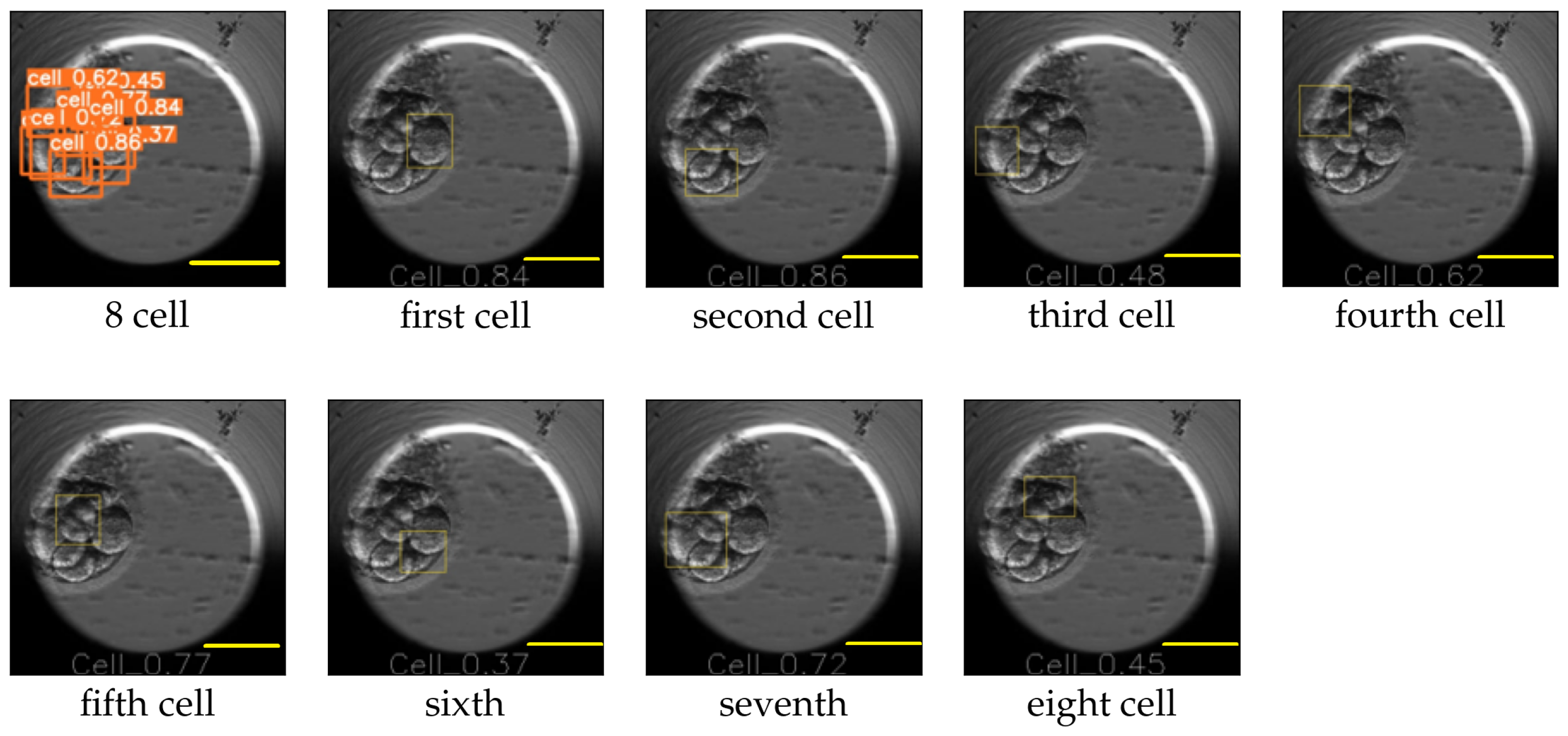
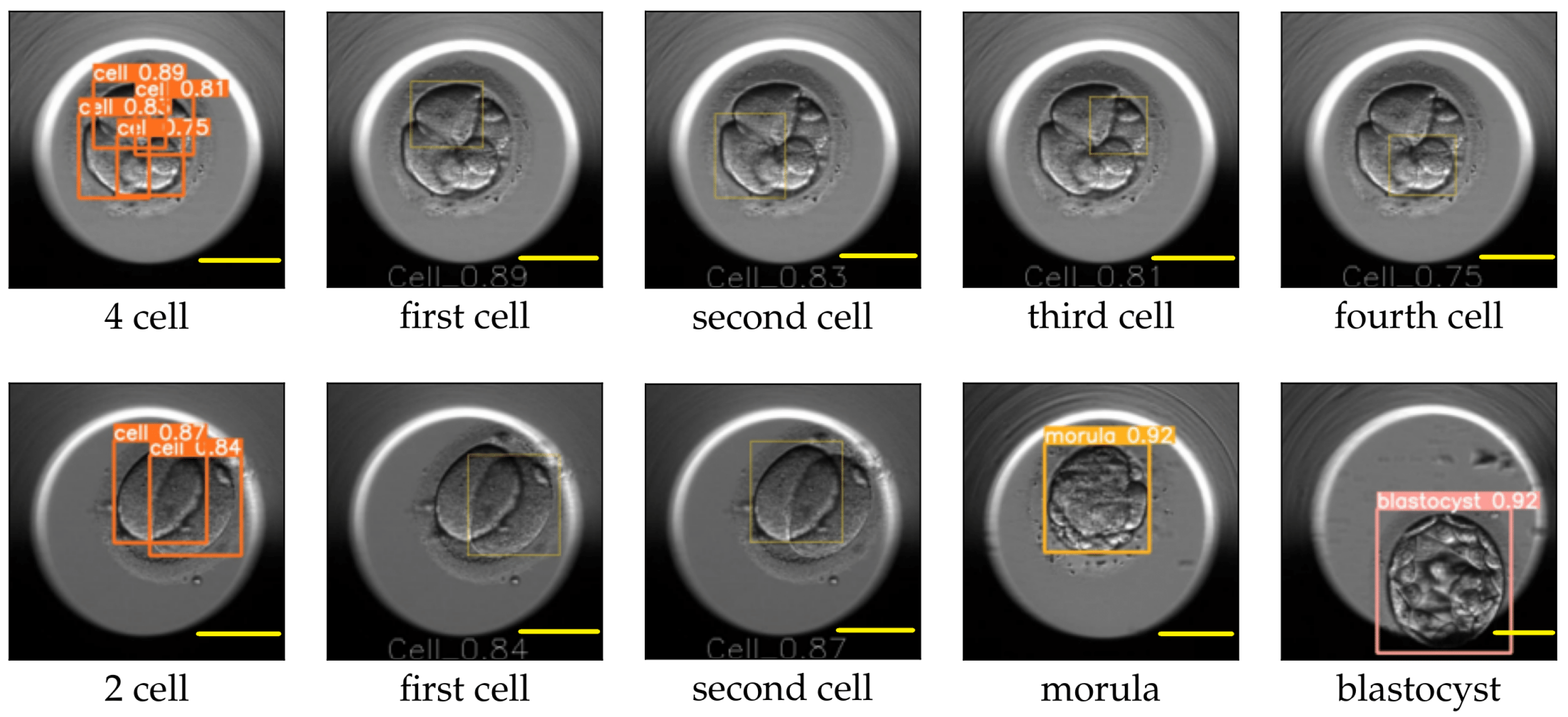
The image size used for training YOLO v5 was 416 × 416, and the value for the hyperparameter determining the minimum bounding box confidence score was 0.30. YOLO v5 reported the mAP for the cell, morula, and blastocyst equal to 0.65, 0.78, and 0.80, respectively. An example of the YOLO predictions for the eight-cell, four-cell, two-cell, morula, and blastocyst stages is explained in Figure 10 and Figure 11. The figures replicate the input image and draw each bounding box separately along with the class probability of the detection.

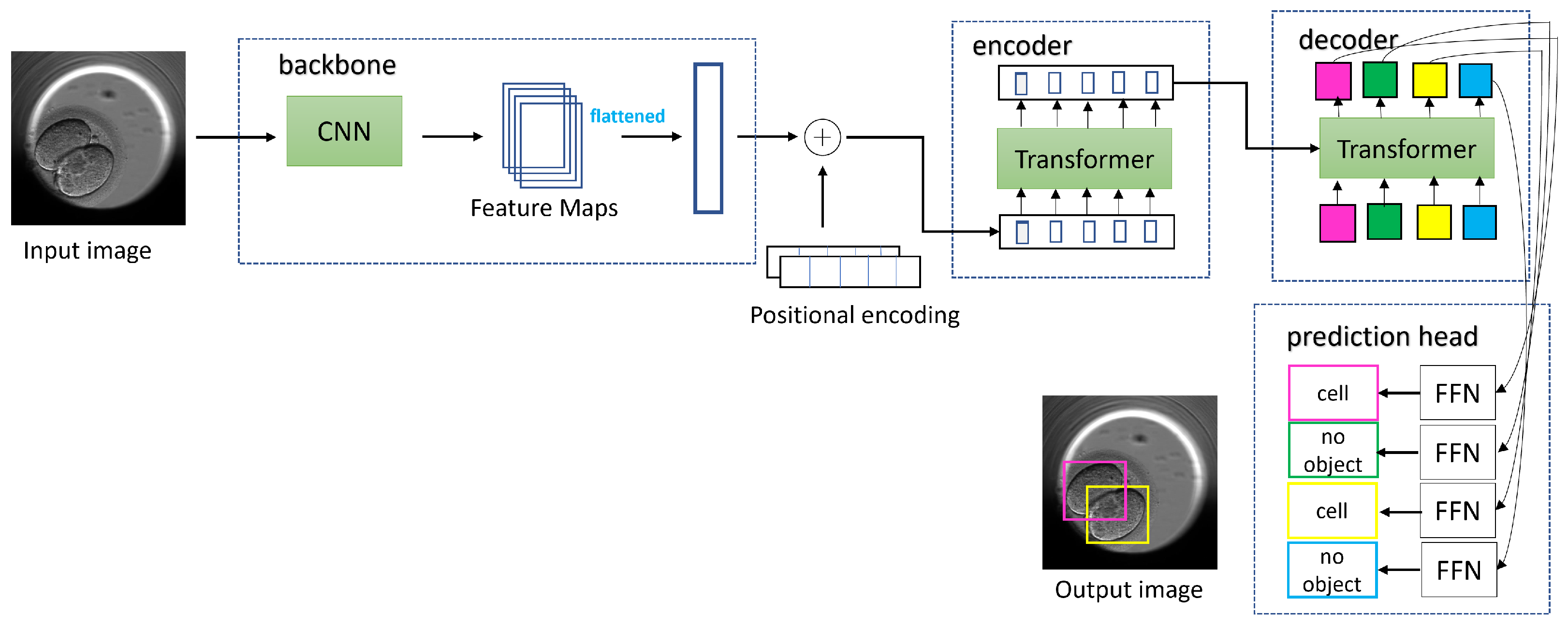
To train the DETR model, we followed a multistep process. Initially, we set the image size to 416 × 416 and the batch size to eight. During training, we updated the gradients after every four batches, which was equivalent to 32 images. We replaced the last layer of the model (FFN) with a custom layer that predicted the bounding boxes and class labels for the cells, morula, and blastocysts. In the first ten epochs of training, we froze the backbone (ResNet-50) and the transformer (encoder, decoder) while only training the last layer with a learning rate of 1 × 10⁻³.In the subsequent 50 epochs, we unfroze the transformer and the last layer and only froze the backbone. We continued to train the last layer with the transformer, with learning rates of 1 × 10⁻³ and 1 × 10⁻⁴, respectively. After 60 epochs of training, we achieved an IoU validation loss equal to 0.22, an L1 loss equal to 0.05, and a cross-entropy loss equal to 0.16. For the next 170 epochs, we unfroze all the blocks, including the backbone, transformer, and last layer. We trained the model with learning rates of 1 × 10⁻⁵, 1 × 10⁻⁴, and 1 × 10⁻³ for the backbone, transformer, and last layer, respectively. Finally, after the full training process, we achieved a final IoU validation loss equal to 0.16, an L1 loss equal to 0.04, and a cross-entropy loss equal to 0.14. 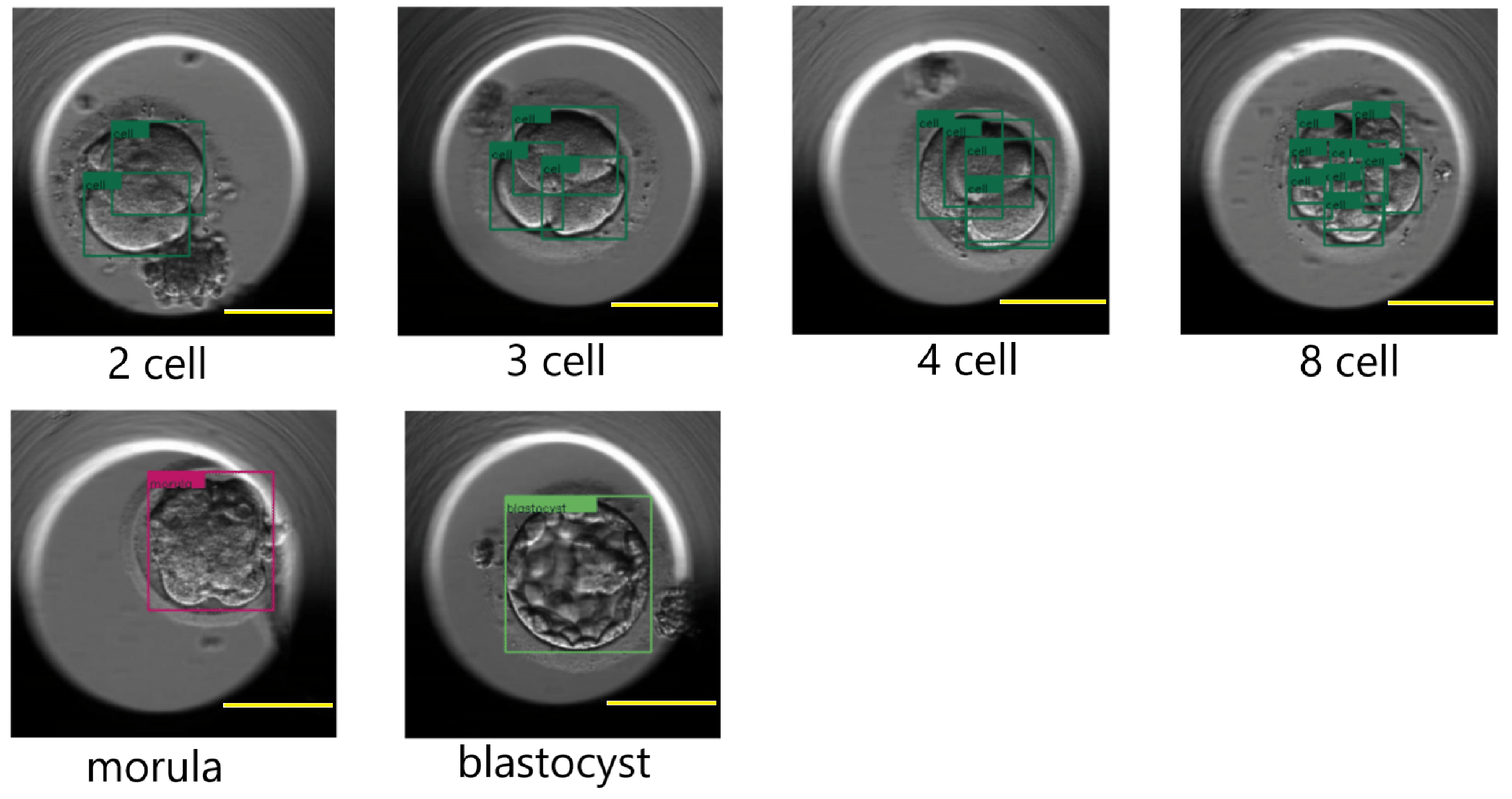Figure 12 shows a few results of the DETR detecting cells, morula, and blastocysts.

5.2. Detecting the Start of Cleavage Stages

In this section, we focus on identifying the cell cleavage stages associated with the objects detected (cells, morula, or blastocyst) in the previous section. The trained object detection algorithms localize the objects in a frame and provide class probabilities for each detected object. The suggested methodology counts the number of detected objects in a frame and maps the frame to the corresponding cell cleavage stage if the class probability of each detected object is above a specified threshold value. The cell count and threshold values are parameters used for predicting the start of the cell cleavage stage. For example, if two cells were detected with each cell class probability above the specified threshold for the two-cell stage, the frame was classified as a two-cell stage.

The threshold values were determined empirically by evaluating the object detection algorithm on the evaluation set of the TransferV dataset. For each frame in the evaluation set, the embryologists evaluated the methodology’s performance and set the threshold values for each cell cleavage stage based on their analysis. The threshold values for the cell cleavage stages were: 0.80 for the two-cell, 0.70 for the three-cell, 0.65 for the four-cell, 0.60 for the five-cell, and 0.50 for the six-cell up to 9+-cell. The threshold value for the morula and blastocyst stages was set to 0.90.

In a video, there can be several frames associated with a cell cleavage stage. Therefore, the methodology organized the frames for each cell cleavage stage, and the first frame from the series was annotated as the start of the cell cleavage stage. The frames put in a series should have matching values for the parameters cell count and threshold. Whether the methodology used YOLO v5 or DETR for the object detection, the same annotation scheme was used. To potentially reduce the noise in the computed probabilities, we also explored using the moving average of the probabilities for three and five subsequent frames, and compared these with the threshold value. However, using the probabilities without averaging turned out to perform better.

5.3. Computing Annotations for the Cleavage Stages Starting Time in hpi

In the previous section, we explained how to find the frame associated with the start of a cleavage stage. In this section, we explain how to find the corresponding time in the hpi. The time corresponds to the occurrence of the captured embryo development in the video recorded in hours (post insemination) by the TLT system. There were two categories of TLT videos: the first one, where the hours were appended to the video frame (as shown in Figure 2) and the second one, where the time entry was missing from the frames. The suggested methodology used the OCR libraries to detect the encoded time when the hpi value was present in the video frames. We evaluated the OCR libraries: Pytesseract, EasyOCR, and Keras-OCR. Recall the introduction to the libraries in Section 3.2. However, for the TLT videos where the frames were not annotated with hpi, the methodology calculated the hours using the duration of the video, the start time of fertilization, the number of frames, and the frame rate of the TLT system.

6. Results

In this Section, we evaluate the performance of the suggested methodology for annotating the start of the cell cleavage stages, both in terms of the frame number and hours. We summarize the performance of the methodology in predicting the start of the cell cleavage stage in Section 6.1 and evaluate the performance in annotating the start time measured in hpi for the observed cell cleavage stages in Section 6.2.

The cell cleavage stages of the morula and blastocyst have unique substages in terms of morphology. As the object detection component of our method was only trained to detect the first substage, we did not evaluate the morula and blastocyst with the other cell cleavage stages. Nevertheless, our method effectively detected the first substages of the morula and blastocyst, and this was independently verified by three embryologists. In the rest of the paper, $Detec{t}_Y$ and $Detec{t}_D$ refer to the suggested methodology to detect the start of a cleavage stage, when YOLO v5 and DETR were used for the object detection, respectively.

6.1. Detecting Cell Cleavage Stages

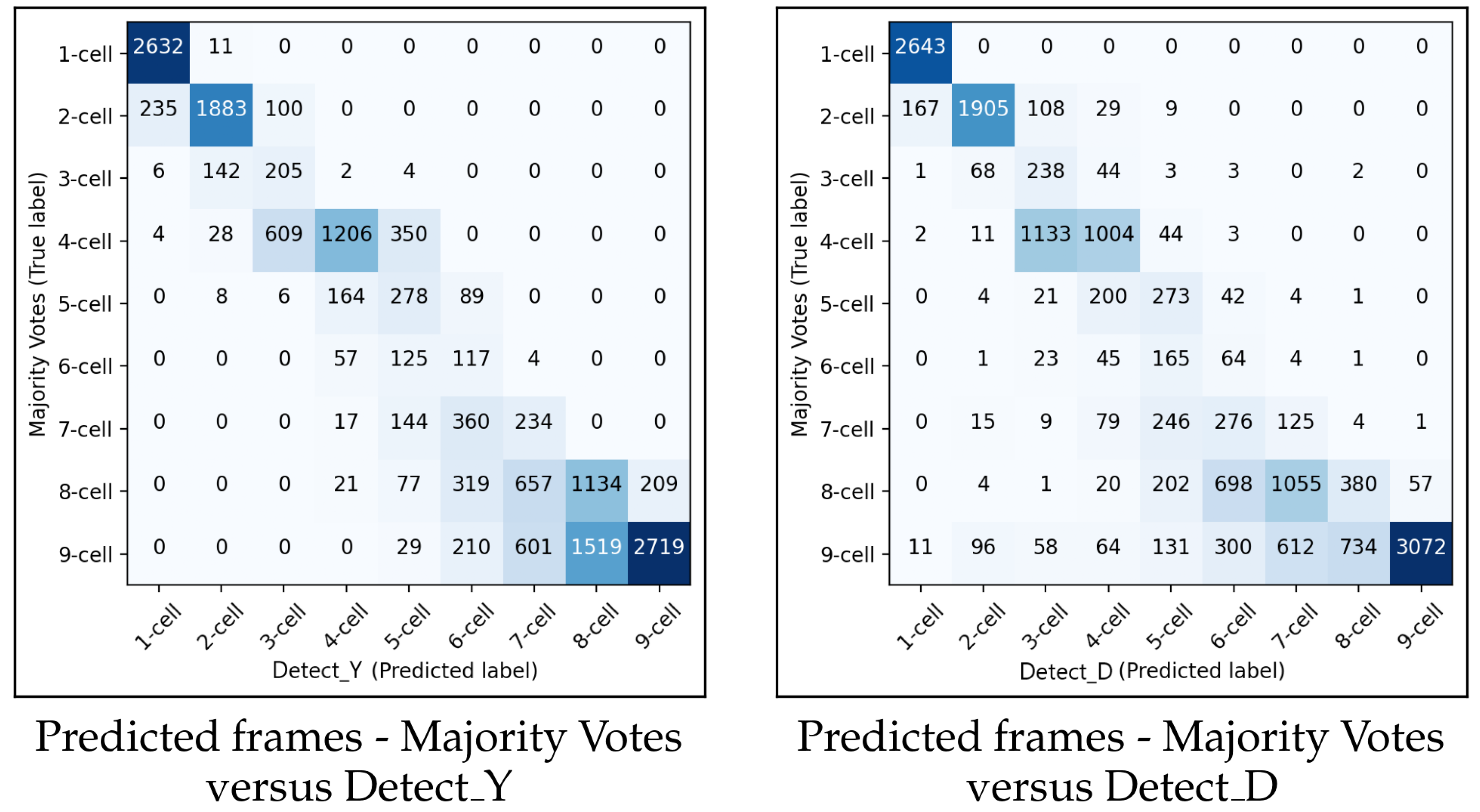
In this Section, we present the evaluation results for the methodology in predicting the starting frame of the cell cleavage stages. The predictions were evaluated on the FrozenV dataset. The performance of the suggested method was compared with the majority vote of the three embryologists, described in Section 4. Figure 13 shows the confusion matrices for $Detec{t}_Y$ and $Detec{t}_D$ for predicting the starting frame of a cleavage stage.

In general, the performances of $Detec{t}_Y$ and $Detec{t}_D$ were similar. When the methodology made a wrong prediction, it was mainly with the adjacent cell cleavage stage. Additionally, in most cases when the methodology predicted incorrectly, it predicted too few cells. In the confusion matrix for $Detec{t}_Y$, there were more misclassifications between the eight-cell stage and the adjacent stages of seven cells and nine+ cells compared to the previous cleavage stages. A similar pattern of misclassification was also observed in $Detec{t}_D$.

The methodology was further evaluated using the six performance metrics of precision, recall, specificity, accuracy, F1-score, and the Matthews correlation coefficient (MCC). Each metric evaluates the methodology’s performance on different parameters, providing a reliable and thorough analysis of its predictive capability [49]. Precision quantifies the proportion of the correctly identified starts of the cleavage stages out of all the predicted starts of cleavage stages. Recall computes the ratio of the correctly predicted starts of a cleavage stage to all the predicted start frames indicated by the methodology. The F1-score is the weighted average of the precision and recall. For a cell cleavage stage, the specificity measures the proportion of predictions that were not mislabeled by the methodology as the start of another cell cleavage stage. The MCC metric provides an overall evaluation of the methodology’s accuracy in predicting the start of the cell cleavage stages and avoiding misclassifications with the start of the other cell cleavage stages. The MCC value ranges from −1 to 1, where a negative value indicates disagreement, a positive value indicates agreement, and a zero value indicates no agreement.

Table 4. Performance in predicting the cell cleavage stage on the FrozenV dataset for $Detec{t}_Y$ (upper table) and $Detec{t}_D$ (lower table).

Cell Cleavage Stage	${\mathit{Detect}}_{\mathit{Y}}$
	Precision	Recall	Specificity	Accuracy	F1-Score	MCC
1-cell	0.91	1.00	0.98	0.99	0.95	0.58
2-cell	0.91	0.85	0.99	0.85	0.88
3-cell	0.22	0.57	0.96	0.57	0.32
4-cell	0.82	0.55	0.98	0.55	0.66
5-cell	0.28	0.51	0.95	0.51	0.36
6-cell	0.11	0.39	0.94	0.39	0.17
7-cell	0.16	0.31	0.92	0.31	0.21
8-cell	0.43	0.47	0.89	0.47	0.45
9+-cell	0.93	0.54	0.98	0.54	0.68
Cell Cleavage Stage	${\mathit{Detect}}_{\mathit{D}}$
	Precision	Recall	Specificity	Accuracy	F1-Score	MCC
1-cell	0.94	1.00	0.99	1.00	0.97	0.53
2-cell	0.91	0.86	0.99	0.86	0.88
3-cell	0.15	0.66	0.92	0.66	0.24
4-cell	0.68	0.46	0.97	0.46	0.55
5-cell	0.25	0.50	0.95	0.50	0.34
6-cell	0.05	0.21	0.92	0.21	0.08
7-cell	0.07	0.17	0.89	0.17	0.10
8-cell	0.34	0.16	0.95	0.16	0.21
9+-cell	0.98	0.60	0.99	0.60	0.75

shows the prediction performance of $Detec{t}_Y$ v5 and $Detec{t}_D$ evaluated per cleavage stage.

The methodology performed the best for the one-cell and two-cell stages with consistent and high prediction rates. Specifically, the F1-score for the methodology using $Detec{t}_Y$ was 0.95 and using $Detec{t}_D$ was 0.97 for the one-cell stage, and the F1-score value was 0.88 for the methodology using both $Detec{t}_Y$ and $Detec{t}_D$ for the two-cell stage. Further, both the recall and precision values were high. The methodology demonstrated good prediction performance for the four-cell stage, with an F1-score of 0.66 using $Detec{t}_Y$ and 0.55 using $Detec{t}_D$. However, for the three-cell and five-cell stages, the methodology had lower discriminative ability and reported average recall and low precision values. These stages were also underrepresented compared to the other stages (FrozenV dataset in Figure 9), which might have affected the performance. The methodology’s prediction performance dropped considerably for the six-cell stage and onward, with both recall and precision values decreasing. However, the methodology had high specificity values for all cell stages, indicating lower misclassification rates between different cell cleavage stages.

We conducted a performance analysis comparing the two object detection algorithms used in the methodology. $Detec{t}_Y$ had a higher MCC value of 0.58 compared to 0.53 for $Detec{t}_D$. Additionally, the accuracy rate was lower for $Detec{t}_D$ compared to $Detec{t}_Y$ from the one-cell stages to the eight-cell stages. Thus, the methodology performed better using $Detec{t}_Y$ than using $Detec{t}_D$. Additionally, we evaluated the methodology using two other versions of YOLO: YOLO v5 with soft NMS and YOLO v7. However, these tests did not result in any improvement. In fact, the performance metrics reported by the methodology were lower than those obtained using $Detec{t}_Y$ from the five-cell stage onward.

Recall that Table 3 shows the agreement rate between E1, E2, and E3 on the starting frame for cell cleavage stages. The overall agreement rate was much higher in comparison to the suggested methodology for predicting the starting frame. The average value for E1 was 0.90, E2 was 0.81, and E3 was 0.88. In comparison, the average accuracy rate for $Detec{t}_Y$ was 0.57, and for $Detec{t}_D$, it was 0.51. As mentioned in Section 4, the observed fragmentation in the FrozenV dataset was higher than that of the TransferV dataset, but the change in the fragmentation rate had no consequence on the performance of $Detec{t}_Y$ and $Detec{t}_D$. The embryologists validated that the methodology did not mistakenly identify small-sized fragments as cells, even wjen the fragments had overlapping boundaries with the cells.

6.2. Annotating Hours Post Insemination for the Cell Cleavage Stages

In this section, we address the problem of predicting the time in hpi for the start of a cell cleavage stage. We used OCR to extract the timing information available in the video frames. In the previous section, we observed that $Detec{t}_Y$ performed better than $Detec{t}_D$ and that $Detec{t}_Y$ could efficiently detect the frame marking the start of the cell cleavage stages up to five cells. Therefore, we evaluated the performance of $Detec{t}_Y$ in predicting the time in hpi up to five cells. We evaluated the OCR libraries pytesseract, EasyOCR, and Keras-OCR. We tested the OCR libraries such as pytesseract, EasyOCR, and Keras-OCR for digit recognition (time encoded in frames) and compared their performance against the time annotations obtained through majority voting. In recognizing the time digits present in the frames, pytesseract performed the best. The pytesseract library only confused the digits ‘4’ and ‘1’ in 0.2% of the tests. Both EasyOCR and Keras-OCR wrongly recognized digits as alphabets and with much higher percentages (EasyOCR: 4.8%, Keras-OCR: 3.6%). We also computed the time needed by the different OCR libraries as part of $Detec{t}_Y$ to annotate the whole FrozenV dataset. The annotation task was finished in 8.21 min with pytesseract, 9.09 min with EasyOCR, and 9.22 min with Keras-OCR.

Using $Detec{t}_Y$ with pytesseract, a time delay was observed in predicting the start of the cell cleavage stages compared to the embryologists’ majority votes. The average time delay for the one-cell stage was minimal, 1.24 hpi for the two-cell stage, 0.63 hpi for the three-cell stage, 2.93 hpi for the four-cell stage, and 3.04 hpi for the five-cell stage, showing an increasing trend in the time delay with an increasing number of cells. However, the methodology also detected the starting time in hpi before the embryologists for a few instances of the cell cleavage stages. The embryologists (E1, E2, and E3) manually inspected these cases and found that the most of these instances were in the transition phase or capturing active cell division. The embryologists concluded that the methodology’s prediction was correct around the transition phase, which is also subjective and challenging to annotate. The embryologists further pointed out that the primary reason that the methodology reported time delays was the presence of excessive overlapping between cell membranes in the video. Naturally, the overlapping becomes increasingly challenging with the increasing number of cells in the embryo.

7. Discussion

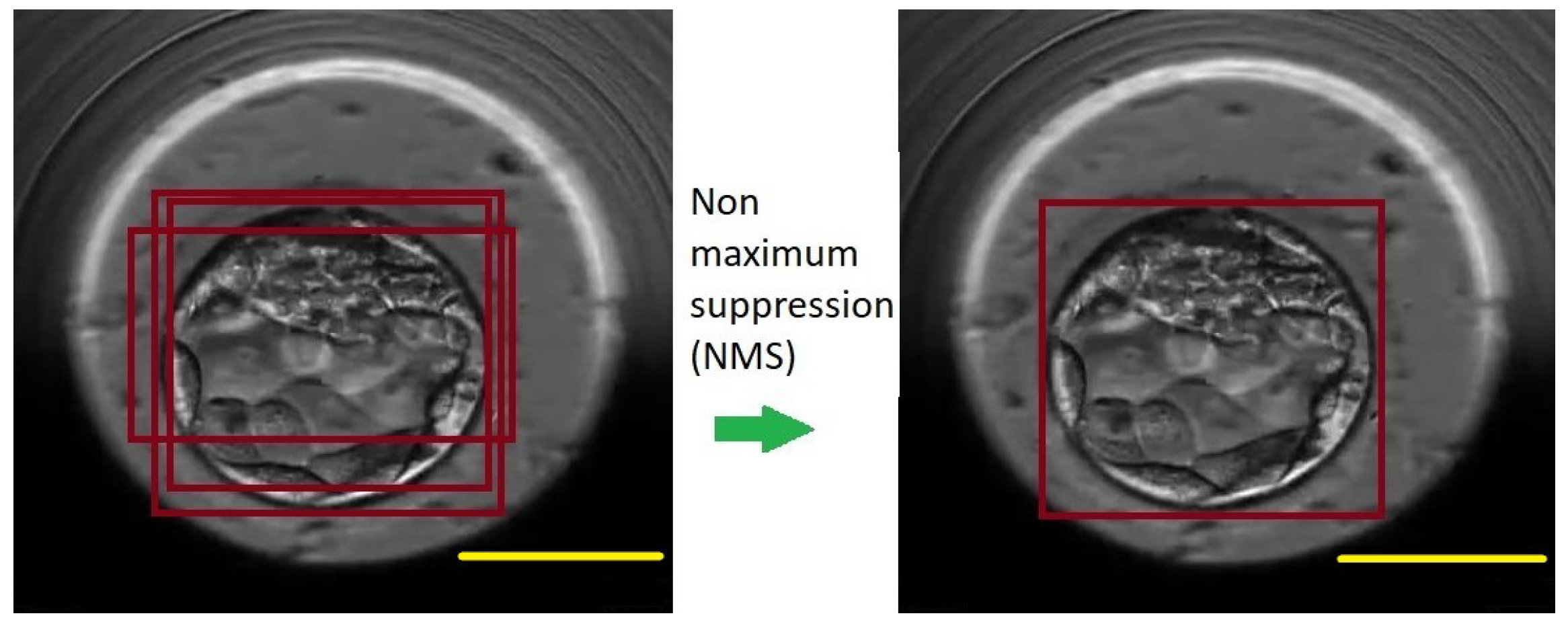
This study aimed to propose a methodology that could help embryologists in clinical settings to annotate the start time of human embryo cell cleavage stages post insemination. Evaluating the quality of embryos involves analyzing the time duration of different cleavage stages, and automating the process of time computation would be useful. Our presented methodology can detect the starting time for cell cleavage stages up to five cells with a delay of 2–3 h post insemination (hpi). When the cell count during cleavage stages was higher than five, the methodology experienced a significant time delay compared to the majority of votes from embryologists. This was because there was excessive overlapping between cell boundaries, which became more noticeable as the number of cells increased. This overlapping led to a lower performance of the methodology, and the embryologists confirmed that cell counting becomes difficult when there is excessive overlapping, resulting in higher disagreement amongst themselves. To address the cell counting issue amidst overlapping, a direction for future work is to train the object detection algorithms specifically on frames of cleavage stages with high overlapping between cells. Among the object detection algorithms tested, YOLO v5 outperformed DETR. YOLO employs non-maximum suppression (NMS) to suppress the bounding boxes with high overlapping areas, which could potentially explain its difficulty in detecting distinct cells with overlapping boundaries. The strategy to redesign NMS with soft-NMS also proved to be ineffective. In future studies, we plan to investigate the methodology using YOLO v5 with adaptive NMS or using Confluence [50] as an alternative to NMS to detect the start of the cell cleavage stages with cell counts greater than five.

The methodology using DETR performed the best when each of the DETR’s architectural blocks were separately finetuned during training. When it comes to detecting cells, the performance of the DETR was only slightly less accurate than that of the YOLO. However, the results might improve further if we trained on more data. Additionally, our methodology used a parameter called “threshold” in predicting the start of a cell cleavage stage and its value was determined empirically after evaluating a small dataset. Therefore, having access to more data could help in providing a more accurate estimate of the true value of this parameter. During the division of an embryo cell, some of the cell’s cytoplasm content is not captured by the daughter cells and instead becomes extracellular material or fragments. The rate of fragmentation can affect the performance of our methodology because these fragments can be mistaken for cells. Our suggested methodology analyzed raw TLT video frames without any image processing to remove fragments, so we evaluated its performance against the fragmentation present in the datasets. This evaluation is relevant for clinical settings as well. We found that the methodology correctly identified cells and did not confuse them with fragments, despite the fact that both datasets (TransferV and FrozenV) contained TLT videos with a range of low to high fragmentation rates. However, the sizes of the fragments in these datasets was small to medium. To fully validate the methodology for clinical use, there is a need to evaluate the methodology’s performance also for larger-sized fragments. The methodology accurately detected the structure of the morula and blastocyst cell cleavage states. This is also relevant for clinical use. As a future research direction, we recommend to train the methodology to detect the start of substages for morula (start of compaction) and blastocyst (start, full blastocyst, expansion, and hatching).

The TLT video frames capturing the embryo development only provide two-dimensional images. This imaging limitation results in a loss of depth information regarding the three-dimensional embryo cell structure, making it difficult to identify overlapping cells. To overcome this challenge, we suggest exploring other imaging modalities instead of using time-lapse systems. Currently, the methodology can only predict the start time (in hours post insemination (hpi)) of cell cleavage stages and only for TLT videos. Whether the methodology calculates the hpi or reads it from the video frames, the computation of time is dependent on the time-lapse system. Therefore, switching to a different imaging modality would require updating the methodology to ensure that the time computation for hpi remains accurate.

8. Conclusions

The timing between successive cell cleavages serves as a reliable and noninvasive marker for predicting human embryo viability. Automating the tracking of cell divisions can provide embryologists with valuable insights into embryo development and implantation potential. Our proposed methodology efficiently detected the start of consecutive cell cleavage stages in TLT videos up to the five-cell stage, with an average time delay of 2–3 hpi. Excessive overlapping of cell boundaries led to delays and decreased the performance in detecting the start of later cell cleavage stages (cell count greater than five). However, our methodology accurately detected the distinct structures of cell cleavage stages, such as the morula and blastocyst.

Our approach successfully distinguished between cells and small-sized fragments with overlapping boundaries, preventing the misclassification of fragments as cells. The methodology’s pipeline performed best when YOLO v5 was used for detecting cells, morula, and blastocysts in the TLT video frames and with Pytesseract as the OCR library for reading out time digits. The methodology computed annotations for TLT videos in real time, with the overall computation time for annotating a video being approximately one minute.

For future work, we suggest investigating the latest developments in deep-neural-network-based image analysis to improve the cell detection in overlapping regions. This could involve training object detection algorithms on frames with a high degree of cell overlap, exploring alternative imaging modalities for capturing three-dimensional embryo cell structures, and employing advanced deep learning techniques, such as transformers and capsule networks, to enhance the performance of our methodology in detecting the start of cell cleavage stages with cell counts greater than five.

References

1. Kan-Tor, Y.; Zabari, N.; Erlich, I.; Szeskin, A.; Amitai, T.; Richter, D.; Or, Y.; Shoham, Z.; Hurwitz, A.; Har-Vardi, I.; et al. Automated Evaluation of Human Embryo Blastulation and Implantation Potential using Deep-Learning. Adv. Intell. Syst. 2020, 2, 2000080. [Google Scholar] [CrossRef]
2. Kragh, M.F.; Rimestad, J.; Lassen, J.T.; Berntsen, J.; Karstoft, H. Predicting Embryo Viability Based on Self-Supervised Alignment of Time-Lapse Videos. IEEE Trans. Med. Imaging 2022, 41, 465–475. [Google Scholar] [CrossRef] [PubMed]
3. Gardner, D.; Schoolcraft, W. In vitro culture of human blastocysts. In Towards Reproductive Certainty: Infertility and Genetics Beyond; Parthenon Press: Carnforth, UK, 1999; pp. 378–388. [Google Scholar]
4. Meseguer, M.; Herrero, J.; Tejera, A.; Hilligsøe, K.M.; Ramsing, N.B.; Remohí, J. The use of morphokinetics as a predictor of embryo implantation†. Hum. Reprod. 2011, 26, 2658–2671. [Google Scholar] [CrossRef] [PubMed]
5. Alpha Scientists in Reproductive Medicine; ESHRE Special Interest Group of Embryology. The Istanbul consensus workshop on embryo assessment: Proceedings of an expert meeting †. Hum. Reprod. 2011, 26, 1270–1283. [Google Scholar] [CrossRef] [PubMed]
6. Baczkowski, T.; Kurzawa, R.; Głabowski, W. Methods of scoring in in vitro fertilization. Reprod. Biol. 2004, 4, 5–22. [Google Scholar]
7. Van Royen, E.; Mangelschots, K.; De Neubourg, D.; Valkenburg, M.; Van de Meerssche, M.; Ryckaert, G.; Eestermans, W.; Gerris, J. Characterization of a top quality embryo, a step towards single-embryo transfer. Hum. Reprod. 1999, 14, 2345–2349. [Google Scholar] [CrossRef]
8. Aparicio, B.; Cruz, M.; Meseguer, M. Is morphokinetic analysis the answer? Reprod. Biomed. Online 2013, 27, 654–663. [Google Scholar] [CrossRef]
9. Wong, C.C.; Loewke, K.E.; Bossert, N.L.; Behr, B.; De Jonge, C.J.; Baer, T.M.; Pera, R.A.R. Non-invasive imaging of human embryos before embryonic genome activation predicts development to the blastocyst stage. Nat. Biotechnol. 2020, 28, 1115–1121. [Google Scholar] [CrossRef]
10. Milewski, R.; Ajduk, A. Time-lapse imaging of cleavage divisions in embryo quality assessment. Reproduction 2017, 154, R37–R53. [Google Scholar] [CrossRef]
11. Dal Canto, M.; Coticchio, G.; Mignini Renzini, M.; De Ponti, E.; Novara, P.V.; Brambillasca, F.; Comi, R.; Fadini, R. Cleavage kinetics analysis of human embryos predicts development to blastocyst and implantation. Reprod. Biomed. Online 2012, 25, 474–480. [Google Scholar] [CrossRef]
12. Cruz, M.; Garrido, N.; Herrero, J.; Pérez-Cano, I.; Muñoz, M.; Meseguer, M. Timing of cell division in human cleavage-stage embryos is linked with blastocyst formation and quality. Reprod. Biomed. Online 2012, 25, 371–381. [Google Scholar] [CrossRef] [PubMed]
13. Cetinkaya, M.; Pirkevi, C.; Yelke, H.; Colakoglu, Y.K.; Atayurt, Z.; Kahraman, S. Relative kinetic expressions defining cleavage synchronicity are better predictors of blastocyst formation and quality than absolute time points. J. Assist. Reprod. Genet. 2015, 32, 27–35. [Google Scholar] [CrossRef] [PubMed]
14. Sakkas, D.; Shoukir, Y.; Chardonnens, D.; Bianchi, P.; Campana, A. Early cleavage of human embryos to the two-cell stage after intracytoplasmic sperm injection as an indicator of embryo viability. Hum. Reprod. (Oxf. Engl.) 1998, 13, 182–187. [Google Scholar] [CrossRef]
15. Shoukir, Y.; Campana, A.; Farley, T.; Sakkas, D. O-225. Early cleavage of in-vitro fertilized human embryos to the 2-cell stage: A novel indicator of embryo quality and viability. Hum. Reprod. 1997, 12, 111. [Google Scholar] [CrossRef]
16. Doronin, Y.K.; Senechkin, I.V.; Hilkevich, L.V.; Kurcer, M.A. Cleavage of Human Embryos: Options and Diversity. Acta Nat. 2016, 8, 88–96. [Google Scholar] [CrossRef]
17. Raudonis, V.; Paulauskaite-Taraseviciene, A.; Sutiene, K.; Jonaitis, D. Towards the automation of early-stage human embryo development detection. Biomed. Eng. OnLine 2019, 18, 120. [Google Scholar] [CrossRef] [PubMed]
18. Riegler, M.; Stensen, M.; Witczak, O.; Andersen, J.; Hicks, S.; Hammer, H.; Delbarre, E.; Halvorsen, P.; Yazidi, A.; Holst, N.; et al. Artificial intelligence in the fertility clinic: Status, pitfalls and possibilities. Hum. Reprod. 2021, 36, 2429–2442. [Google Scholar] [CrossRef] [PubMed]
19. Khosravi, P.; Kazemi, E.; Zhan, Q.; Malmsten, J.E.; Toschi, M.; Zisimopoulos, P.; Sigaras, A.; Lavery, S.; Cooper, L.A.D.; Hickman, C.; et al. Deep learning enables robust assessment and selection of human blastocysts after in vitro fertilization. NPJ Digit. Med. 2019, 2, 21. [Google Scholar] [CrossRef] [PubMed]
20. Tran, D.; Cooke, S.; Illingworth, P.J.; Gardner, D.K. Deep learning as a predictive tool for fetal heart pregnancy following time-lapse incubation and blastocyst transfer. Hum. Reprod. (Oxf. Engl.) 2019, 34, 1011–1018. [Google Scholar] [CrossRef]
21. Li, Z.; Dong, M.; Wen, S.; Hu, X.; Zhou, P.; Zeng, Z. CLU-CNNs: Object detection for medical images. Neurocomputing 2019, 350, 53–59. [Google Scholar] [CrossRef]
22. Al-masni, M.; Al-antari, M.A.; Park, J.; Gi, G.; Kim, T.; Rivera, P.; Valarezo Añazco, E.; Han, S.M.; Kim, T.S. Detection and Classification of the Breast Abnormalities in Digital Mammograms via Regional Convolutional Neural Network. In Proceedings of the 2017 39th Annual International Conference of the IEEE Engineering in Medicine and Biology Society (EMBC), Seogwipo, Republic of Korea, 11–15 July 2017. [Google Scholar] [CrossRef]
23. Jha, D.; Ali, S.; Tomar, N.K.; Johansen, H.D.; Johansen, D.; Rittscher, J.; Riegler, M.A.; Halvorsen, P. Real-Time Polyp Detection, Localization and Segmentation in Colonoscopy Using Deep Learning. IEEE Access 2021, 9, 40496–40510. [Google Scholar] [CrossRef] [PubMed]
24. Pogorelov, K.; Riegler, M.; Eskeland, S.; de Lange, T.; Johansen, D.; Griwodz, C.; Schmidt, P.; Halvorsen, P. Efficient disease detection in gastrointestinal videos–Global features versus neural networks. Multimed. Tools Appl. 2017, 76, 22493–22525. [Google Scholar] [CrossRef]
25. Wright, G.; Wiker, S.; Elsner, C.; Kort, H.; Massey, J.; Mitchell, D.; Toledo, A.; Cohen, J. Observations on the morphology of pronuclei and nucleoli in human zygotes and implications for cryopreservation. Hum. Reprod. 1990, 5, 109–115. [Google Scholar] [CrossRef] [PubMed]
26. Oh, S.; Gong, S.P.; Lee, S.; Lee, E.J.; Lim, J. Light intensity and wavelength during embryo manipulation are important factors for maintaining viability of preimplantation embryos in vitro. Fertil. Steril. 2007, 88, 1150–1157. [Google Scholar] [CrossRef]
27. Ciray, H.N.; Campbell, A.; Agerholm, I.E.; Aguilar, J.; Chamayou, S.; Esbert, M.; Sayed, S. Proposed guidelines on the nomenclature and annotation of dynamic human embryo monitoring by a time-lapse user group. Hum. Reprod. 2014, 29, 2650–2660. [Google Scholar] [CrossRef]
28. Kajhøj, T.Q. iDAScore–The Future of AI-Based Embryo Evaluation. 2020. Available online: https://blog.vitrolife.com/togetheralltheway/idascore-the-future-of-ai-based-embryo-evaluation (accessed on 5 March 2023).
29. Flaccavento, G.; Lempitsky, V.S.; Pope, I.; Barber, P.R.; Zisserman, A.; Noble, J.A.; Vojnovic, B. Learning to Count Cells: Applications to lens-free imaging of large fields. In Proceedings of the Sixth International Workshop on Microscopic Image Analysis with Applications in Biology, Heidelberg, Germany, 2 September 2011. [Google Scholar]
30. Moussavi, F.; Wang, Y.; Lorenzen, P.; Oakley, J.D.; Russakoff, D.B.; Gould, S. A unified graphical models framework for automated human embryo tracking in time lapse microscopy. In Proceedings of the 2014 IEEE 11th International Symposium on Biomedical Imaging (ISBI), Beijing, China, 29 April–2 May 2014; pp. 314–320. [Google Scholar]
31. Khan, A.; Gould, S.; Salzmann, M. Deep Convolutional Neural Networks for Human Embryonic Cell Counting. In Proceedings of the ECCV Workshops (1), Amsterdam, The Netherlands, 8–10 and 15–16 October 2016; pp. 339–348. [Google Scholar]
32. Khan, A.; Gould, S.; Salzmann, M. Automated monitoring of human embryonic cells up to the 5-cell stage in time-lapse microscopy images. In Proceedings of the 2015 IEEE 12th International Symposium on Biomedical Imaging (ISBI), Brooklyn Bridge, NY, USA, 16–19 April 2015; pp. 389–393. [Google Scholar] [CrossRef]
33. Khan, A.; Gould, S.; Salzmann, M. A Linear Chain Markov Model for Detection and Localization of Cells in Early Stage Embryo Development. In Proceedings of the 2015 IEEE Winter Conference on Applications of Computer Vision, Waikoloa, HI, USA, 5–9 January 2015; pp. 526–533. [Google Scholar] [CrossRef]
34. Xie, W.; Noble, J.A.; Zisserman, A. Microscopy cell counting and detection with fully convolutional regression networks. Comput. Methods Biomech. Biomed. Eng. Imaging Vis. 2018, 6, 283–292. [Google Scholar] [CrossRef]
35. Brownlee, J. A Gentle Introduction to Object Recognition with Deep Learning. 2019. Available online: https://machinelearningmastery.com/object-recognition-with-deep-learning/ (accessed on 13 March 2023).
36. Bandyopadhyay, H. YOLO: Real-Time Object Detection Explained. 2020. Available online: https://towardsdatascience.com/real-time-object-detection-pytorch-yolo-f7fec35afb64 (accessed on 11 January 2023).
37. Redmon, J.; Divvala, S.; Girshick, R.; Farhadi, A. You Only Look Once: Unified, Real-Time Object Detection. In Proceedings of the 2016 IEEE Conference on Computer Vision and Pattern Recognition (CVPR), Las Vegas, NV, USA, 27–30 June 2016; pp. 779–788. [Google Scholar] [CrossRef]
38. Carion, N.; Massa, F.; Synnaeve, G.; Usunier, N.; Kirillov, A.; Zagoruyko, S. End-to-End Object Detection with Transformers. In Proceedings of the Computer Vision–ECCV 2020: 16th European Conference, Glasgow, UK, 23–28 August 2020; Springer International Publishing: Berlin/Heidelberg, Germany, 2020; pp. 213–229. [Google Scholar] [CrossRef]
39. Salau, J.; Krieter, J. Instance Segmentation with Mask R-CNN Applied to Loose-Housed Dairy Cows in a Multi-Camera Setting. Animals 2020, 10, 2402. [Google Scholar] [CrossRef]
40. Hoffstaetter, S. Python-Tesseract. Software. 2014. Available online: https://github.com/madmaze/pytesseract (accessed on 2 November 2022).
41. AI, J. EasyOCR. Software. 2020. Available online: https://jaided.ai/easyocr/ (accessed on 5 November 2022).
42. Keras-OCR. Software. 2020. Available online: https://github.com/faustomorales/keras-ocr (accessed on 5 November 2022).
43. Jan Zdenek, D.C. Convolutional Recurrent Neural Network for Scene Text Recognition or OCR in Keras. Software. 2019. Available online: https://github.com/janzd/CRNN (accessed on 22 February 2023).
44. Baek, Y.; Lee, B.; Han, D.; Yun, S.; Lee, H. Character Region Awareness for Text Detection. Software. 2019. Available online: https://github.com/clovaai/CRAFT-pytorch (accessed on 22 February 2023).
45. ESHRE Working Group on Time-Lapse Technology; Apter, S.; Ebner, T.; Freour, T.; Guns, Y.; Kovacic, B.; Le Clef, N.; Marques, M.; Meseguer, M.; Montjean, D.; et al. Good practice recommendations for the use of time-lapse technology †. Hum. Reprod. Open 2020, 2020, hoaa008. [Google Scholar] [CrossRef]
46. Kovacs, P. Embryo selection: The role of time-lapse monitoring. Reprod. Biol. Endocrinol. RB&E 2014, 12, 124. [Google Scholar] [CrossRef]
47. LabelBox. Software. Available online: https://labelbox.com/ (accessed on 5 March 2023).
48. Dwyer, B.; Nelson, J. Roboflow (Version 1.0). Software. 2022. Available online: https://roboflow.com/ (accessed on 5 March 2023).
49. Koyejo, O.O.; Natarajan, N.; Ravikumar, P.K.; Dhillon, I.S. Consistent binary classification with generalized performance metrics. Advances in Neural Information Processing Systems, Neural Information Processing Systems 27 (NeurIPS). 2014. Available online: https://proceedings.neurips.cc/paper_files/paper/2014/file/30c8e1ca872524fbf7ea5c519ca397ee-Paper.pdf (accessed on 19 January 2023).
50. Shepley, A.; Falzon, G.; Kwan, P. Confluence: A Robust Non-IoU Alternative to Non-Maxima Suppression in Object Detection. arXiv 2022, arXiv:cs.CV/2012.00257. [Google Scholar] [CrossRef]
Figure 1. Cell cleavage stages of human embryo development. Scale bar: 100 μm.
Bdcc 07 00091 g001
Figure 2. An overview of the methodology’s pipeline predicting the start time of the cell cleavage stages observed in time-lapse videos. Subfigure (A) shows a block diagram of the methodology’s workflow starting with the input of a video through to the methodology predicting time annotations in hpi for the observed cell cleavage stages in the video. Subfigure (B) shows a video frame with time appended in the bottom right corner. The time is read out by OCR, and the suggested methodology provides the annotation pairing cleavage stage and the detected time.
Bdcc 07 00091 g002
Figure 3. Intersection over union (IoU) for bounding boxes. (A) The IoU is calculated by dividing the intersection of the two boxes by the union of the boxes. The intersection region is shaded with blue lines; (B) examples for different values of IoU. Image inspired from the original image in [39].
Bdcc 07 00091 g003
Figure 4. YOLO v5 detects three bounding boxes for the morula stage. The bounding boxes localizing morula are marked in red color. With the use of NMS, YOLO v5 selects the best candidate for the bounding box for the morula object after eliminating the other two boxes. Scale bar: 100 μm.
Bdcc 07 00091 g004
Figure 5. DETR: bipartite matching loss to find the best match between the ground truth and the predicted set of box coordinates and object class predictions. Each detected object is marked with different and unique colored bounding box in square shape. Image inspired from the original paper [38].
Bdcc 07 00091 g005
Figure 6. For an input image, the DETR uses a CNN backbone to obtain the feature maps, which are flattened and supplemented with positional encoding. The input is then fed to a transformer encoder network with multihead attention. The output from the encoder is passed to the transformer decoder and is processed further with the application of learned positional encoding called object queries. The output embedding from the decoder is passed in parallel to the shared feed forward network (FFN) to obtain bounding boxes and classes for the detected objects. Each detected object such as instances of cell class or no-object class are marked with different and unique colored bounding box in square shape. Image inspired from the original paper [38].
Bdcc 07 00091 g006
Figure 7. The schematic design of a time-lapse incubator system. The image draws inspiration from the original image in [17].
Bdcc 07 00091 g007
Figure 8. The top row shows actual images of cleavage stages. The bottom row from left to right shows Labelbox annotations for cells in the two-cell, four-cell, eight-cell, morula, and blastocyst cleavage stages. The bounding boxes annotation for class cell is marked in blue, class morula in red and class blastocyst in purple. Scale bar: 100 μm.
Bdcc 07 00091 g008
Figure 9. Total number of frames in the videos belonging to the different cell cleavage states. The top panel shows the TransferV dataset with the left (a) showing the training set and the right (b) showing the evaluation set. The bottom panel (c) shows the FrozenV dataset.
Bdcc 07 00091 g009
Figure 10. Eight-cell cleavage stage processed by YOLO v5. The first image contains the bounding boxes along with the probabilities of the detected cells. The following images mark the location of each detected cell individually. Scale bar: 100 μm.
Bdcc 07 00091 g010
Figure 11. Cleavage stages: four-cell, two-cell, morula, and blastocyst as processed by YOLO v5. The leftmost image on the top row shows the bounding boxes along with the probabilities of the detected cells for the four-cell stage. The following images mark the location of each detected cell individually. The leftmost image on the bottom row shows the bounding boxes along with the detected cell probabilities for the two-cell stage, followed by images marking the location of the detected cells individually. The last two images correspond to the detection results for the morula and blastocyst. Scale bar: 100 μm.
Bdcc 07 00091 g011
Figure 12. Cleavage stages: two-cell, three-cell, four-cell, eight-cell, morula, and blastocyst as processed by the DETR. The detected cells are marked in a dark green color for the two-cell, three-cell, four-cell and eight-cell images. The morula and blastocyst stages are marked with the colors magenta and light green, respectively. Scale bar: 100 μm.
Bdcc 07 00091 g012
Figure 13. The left and the right panels show the confusion matrices between the embryologists majority votes and D e t e c t Y and D e t e c t D , respectively.
Bdcc 07 00091 g013