Article

Fast and Effective Retrieval for Large Multimedia Collections

1
Faculty of Mathematics and Computer Science, University of Hagen, Universitätsstrasse 1, D-58097 Hagen, Germany
2
Academy for International Science & Research (AISR), Derry BT48 7JL, UK
*
Author to whom correspondence should be addressed.
Big Data Cogn. Comput. 2021, 5(3), 33; https://doi.org/10.3390/bdcc5030033
Submission received: 15 June 2021 / Revised: 7 July 2021 / Accepted: 12 July 2021 / Published: 22 July 2021
(This article belongs to the Special Issue Multimedia Systems for Multimedia Big Data)

Abstract

:
The indexing and retrieval of multimedia content is generally implemented by employing feature graphs. These graphs typically contain a significant number of nodes and edges to reflect the level of detail in feature detection. A higher level of detail increases the effectiveness of the results, but also leads to more complex graph structures. However, graph traversal-based algorithms for similarity are quite inefficient and computationally expensive, especially for large data structures. To deliver fast and effective retrieval especially for large multimedia collections and multimedia big data, an efficient similarity algorithm for large graphs in particular is desirable. Hence, in this paper, we define a graph projection into a 2D space (Graph Code) and the corresponding algorithms for indexing and retrieval. We show that calculations in this space can be performed more efficiently than graph traversals due to the simpler processing model and the high level of parallelization. As a consequence, we demonstrate experimentally that the effectiveness of retrieval also increases substantially, as the Graph Code facilitates more levels of detail in feature fusion. These levels of detail also support an increased trust prediction, particularly for fused social media content. In our mathematical model, we define a metric triple for the Graph Code, which also enhances the ranked result representations. Thus, Graph Codes provide a significant increase in efficiency and effectiveness, especially for multimedia indexing and retrieval, and can be applied to images, videos, text and social media information.

1. Introduction and Motivation

Multimedia assets such as images, videos, social media posts, texts or audio are deeply integrated into the life of many users. The ease of creating multimedia content, e.g., on smartphones, and publishing it on social media has not been evident heretofore. Infrastructure services such as high-speed networks, cloud services or online storage require an efficient and effective structuration of multimedia content [1] because, e.g., every single minute, 147,000 photos are uploaded to Facebook, 41.6 million WhatsApp messages are sent and 347,000 stories are posted by Instagram [2]. These figures are still increasing and leave many open challenges for both users and content providers.
Indexing and fast retrieval of these assets are essential for managing this large volume of information. For this task, graph-based technologies and structures are commonly used, as feature information is based on information nodes and links between these nodes [3]. Such graph structures typically grow significantly and can contain about 500 nodes and 2000 edges per asset. To increase the accuracy of retrieval, more information from various sources (e.g., social media, documents, the Semantic Web, embedded metadata) is integrated into large feature graphs. However, to employ these features, especially for effective retrieval, in a very detailed manner, fast graph-based similarity algorithms are required. Current solutions, as, e.g., Neo4J databases [4], and their integrated algorithms fail to deliver acceptable processing times for retrieval, as they need several minutes to calculate the similarity of fused feature graphs. Typically, response times under 1 s are regarded as “good”, and according to [5], anything over 1s is “a problem”.
In this paper, we describe a fast and accurate retrieval algorithm for multimedia feature graphs and the corresponding mathematical and technical concepts. This algorithm is based on a projection of graphs into a 2D space, which supports parallelization in retrieval and can utilize standard pattern matching algorithms including machine learning. The proposed concept can be applied to any kind of multimedia asset that has a graph representation (e.g., images, videos, text, audio). Especially for multimedia big data, these 2D projections can provide a huge increase in efficiency. For our experiments, we present details on the performance, accuracy and quality based on various datasets, measured on various devices, including tablets. In Section 2, we summarize the current state-of-the-art and related works. Section 3 contains the mathematical and algorithmic details of the Graph Codes and their applications, which form the basis for the implementation given in Section 4. Finally, the evaluation in Section 5 shows the detailed results of the experiments regarding its effectiveness and efficiency. Section 6 concludes and discusses future work.

2. State-of-the-Art and Related Work

This section provides an overview of current indexing and retrieval techniques, which either represent or contribute to the feature information of multimedia content. The indexing and retrieval of textual information, images, audio and video assets are described, and the current concepts for feature integration, which result in large graph structures. The technologies discussed can contribute multimedia features to feature vectors. A brief description of the mathematical background of these graphs is given, and an overview of current datasets for indexing and retrieval.

2.1. Multimedia Feature Extraction

This subsection describes briefly some of the underlying algorithms that can extract or generate features (note: feature categories resulting from the processing of the presented algorithms are given in italics) from varied multimedia content. Comprehensive overviews were given in [6,7,8], and the following presents some selected algorithms and technologies. These algorithms were selected because they extract various mentioned features at different levels from multimedia objects and because they are highly cited in the literature.
Text: For multimedia processing, textual information is usually added in form of metadata, annotations or corresponding short texts (e.g., social media posts, descriptions, tag lines). Typically, for this type of text, the basic Boolean algorithm [8] has provided the best results, as it is specifically designed for small text patterns [9]. Thus, this algorithm is often used when fusing textual information into multimedia feature graphs as discussed in [8]. The normalization and aggregation of texts and result fusion are described in [10].
Images: In addition to the textual processing of an image’s annotations, algorithms for colour-based feature detection using histograms (e.g., dominant colours) or colour distributions of images can provide information in order to identify similar images [8] or regions. Image feature retrieval based on shape, also known as object detection, utilizes edge detection, template matching and rotational normalization to identify if an asset contains one or more detectable objects [6,11]. This also includes, e.g., label detection, text recognition or landmark detection. Algorithms to detect spatial relations (e.g., relationships) [12], and machine learning are often employed to increase the effectiveness of feature detection [6]. Image metadata such as EXIF [13] are also relevant features (e.g., geolocation, date, time, camera model).
Audio: Hidden Markov models (HMMs) are a common basis for several audio algorithms. These models can be split into two categories: (1) forward algorithms (which work well with isolated words) and (2) Viterbi algorithms (for continuous speech). These algorithms are used for speech recognition and analysis and provide a basis for transcribing and textually processing audio content into features. Also, in this field, the use of machine learning (particularly neural networks) has increased the effectiveness of retrieval, but extensive training is required  [9,11,14]. The textual representation of audio is often regarded as a multimedia feature representation [8] and processed with text feature-extraction algorithms.
Video: for indexing videos, several approaches are common: r-frame detection is used to capture the main content of a scene (e.g., main objects, scene type). Features can then be extracted based on image indexing. Shot Detection (i.e., the automated detection of different scenes in video content), can be performed by various algorithms [15]. Motion Information Algorithms extend this detection and also consider motion information  [8,16]. Metadata and Annotations of video are standardized (e.g., MPEG7 [17] with metadata, time codes) and can be used to extract features of the whole video or single shots [9].
In general, every detected feature can be regarded as a multimedia indexing term. The indexing term of any relevant feature thus becomes part of the vocabulary of the overall retrieval index. In Multimedia Indexing and Retrieval (MMIR), these terms typically have structural and/or semantic relationships to each other. Thus, graph-based structures are appropriate candidates to represent multimedia features including their relationships.
To fuse and integrate all of these features, a unifying framework is required. For example, Jean-Baptiste et al. [18] discusses a framework utilizing various sources of video-content (video, audio, and language streams) being fed into a self-supervised multimodal versatile network, which is can enrich information of these various sources. However, frameworks that fuse and integrate features of non-combined multimedia assets (i.e., videos, images, audio, and texts from different sources), rarely exist. Hence, our previous work [19,20,21,22] introduced and implemented a Generic Multimedia Annotation Framework (GMAF), which provides an extendable representation schema and processing architecture for fusing detected multimedia features and generating Multimedia Feature Graph (MMFG) data structures. A detailed definition of the MMFG is given in [22] and the most relevant objectives are outlined in the next section.

2.2. The Multimedia Feature Graph

The Multimedia Feature Graph (MMFG) is a weighted and directed graph [23] representing the features of multimedia assets and is defined as M M F G A s s e t = ( N , E ) , where N is the set of nodes and E the set of edges between these nodes. Both N and E are employed to represent special multimedia features and their relationship, that have been detected within an asset (e.g., instances of object, region, colour, or relationship features). The MMFG also fuses the detected information into a single model. A complete description of the MMFG is given in [22], a reference implementation is available on GitHub [20], and a visualization of a small section of a MMFG is shown in Figure 1, which illustrates several feature types in different colours (e.g., detected objects in blue, detected landmarks in yellow, synonyms in green, spacial relationships in red). 
A complex MMFG contains feature representations for example from text (e.g., metadata or Social Media), images (e.g., objects, colours, spacial attributes), video, and audio information (if applicable) and Figure 1 shows an exemplary MMFG snippet, where the following feature categories are visible: object detection, dominant colours, spacial relationships, landmark detection. In general, the MMFG is a typical graph based data-structure for representing multimedia features. In Section 2.3, methods for representing and processing graphs are discussed in more detail.

2.3. Graph Processing

From a mathematical perspective, graphs can be represented typically through their Adjacency Matrix. Based on this, several further transformations can be made. One example for this is the transformation of a graph into a n-dimensional vector-space to allow further operations including similarity calculation [25]. For weighted graphs (e.g., Multimedia Feature Graphs), typically matrices are employed, which extend Adjacency Matrices by the integration of the edges’ weight-information [26], also enabling the application of mathematical concepts to graphs [25], which are called Valuation Matrices in the remainder of this paper. Similarity calculation on matrices can be performed with the Eigenvalue Method [27], which reduces a square matrix M to a single rational number λ by assuming that there exists a vector v with M · v = λ · v . Then, similarity calculations can be performed on λ instead of the whole matrix. However, each mathematical approach usually has a complexity of O ( ( n + e ) 2 ) (n nodes and e edges). Several approaches are described to improve this for a particular set of data or within particular conditions [28,29,30], but the performance of these algorithms for large data structures, like feature graphs of multimedia objects, must still be improved. One approach for this is given in [31], which utilizes a highly scalable GPU-based algorithm to improve the performance of similarity search within graph structures to flatten the exponential growth of graph-based algorithms.
In the remainder of this paper we describe and evaluate the Graph Code Encoding Algorithm, Query Construction, and Retrieval Execution with Graph Codes, as an extension of graph-based Adjacency Matrices for MMIR applications. These algorithms can perform comparison tasks based on graph data in O ( n + e ) , instead of exponential growth.

2.4. Graph Codes and Their Encoding

This section discusses the mathematical and algorithmic concepts of a 2D graph representation and its relevance for MMIR. We have introduced Graph Codes in [22]. They are applicable to any kind of feature graph, but we specifically designed them for MMIR. They should provide a huge benefit in the area or multimedia indexing and retrieval as a technical representation basis for graph algorithms. We use them to represent MMFGs and to transform these into another mathematical space for fast and efficient MMIR.
Our Graph Code Encoding algorithm [22] uses the Valuation Matrix V M of a given MMFG as a basis. It is also possible to calculate Graph Codes based on n-dimensional vector-spaces and a projection of these into a 2D matrix-space, producing a similar result as the algorithm based on the Valuation Matrix. We chose to employ Valuation Matrices, as this approach is expected to require fewer calculations than vector-space transformations. As an example, we employ a small subgraph of the MMFG of Figure 1 containing the most relevant structures to illustrate the concepts presented in this paper. Thus, we define our example-graph M M F G e x as shown in Figure 2.
Valuation Matrices contain one row and column for each node, always resulting in square matrices. Edges incident on nodes n 1 and n 2 are represented in the matrix with their weight or a value of 1 at row n 1 and column n 2 , i.e., position ( n 1 , n 2 ) . In case of the example above, the set of nodes N is given by N = {Person, Head, Human Being, Individual, Hat, above}, represented by a value of 1 in one of the diagonals of the matrix. Thus, the Valuation Matrix V M is defined as (see also Table 1 and Figure 3):
Graph Codes employ a encoding function f e n c , which calculates a numeric value for each non-zero position of a Valuation Matrix based on node or edge type and the corresponding attributes. The function f e n c can be adjusted deliberately to meet the requirements of any application. In the context of this paper, we chose an arbitrary selection of value ranges representing type attributes of nodes and edges for the Graph Code representation. If we apply such a f e n c to the above example (object-node = 1, synonym-node = 2, child-relationship = 3, synonym-relationship = 4, relationship = 5, spacial-relationship-node = 6), the encoded Valuation Matrix V M e n c i.e., the corresponding Graph Code G C is shown in Figure 4 and Table 2, where node representing fields are painted in bold. Node types in Table 2 are coloured according to Figure 1 and represented by the fields in the diagonal of the matrix. Edge types are coloured (3 = orange, 4 = purple, 5 = yellow).
In future encodings, attributes, weights, or other information about nodes and edges can be encoded with more complex functions resulting in arbitrary natural numbers. In our model, we apply the encoding function f e n c to each matrix field and base it on e.g., three-byte-integer values between 0 and 16.7 million (= m a x c in the later equations). The reason for this is that the resulting Graph Codes can then be interpreted as bitmap images, which provides some benefits in visualization during testing, evaluating, and manually proving results. Although in general, f e n c can be arbitrary defined according to the MMIR application’s requirements.
Based on Graph Codes, we introduce algorithms for Query Construction and Query Execution in the modeling section (Section 3) of this paper, which will evaluated in Section 5. To demonstrate their effectiveness and efficiency, fully annotated sample data are required.

2.5. Annotated Sample Datasets

To evaluate multimedia retrieval algorithms, an appropriate set of sample data must be available. As the evaluation has to demonstrate effectiveness, efficiency and quality, we define the following criteria for the identification and selection or the generation of sample datasets:
  • Content description annotations: to determine the effectiveness of an algorithm, a comparison of the detected features with manually approved content description annotations must be possible. Thus, the sample dataset must include correct and complete content description annotations.
  • Level of detail: processing of each sample must produce a high level of detail, which is an important prerequisite for measuring effectiveness. For image or video processing, the resolution is a informative indicator for the resulting level of detail. For audio processing, the bit-rate is a relevant measure for the level of detail.
  • Number of samples: to calculate reliable figures, the dataset has to contain a relevant number of samples to be processed.
To analyze algorithms for multimedia processing, several datasets can be employed. One of the most comprehensive collections of annotated text-based sample data is maintained by the Text Retrieval Conference (TREC) [32], a comprehensive overview of audio datasets (e.g., The Spoken Wikipedia Corpora) is given by [33] and a commonly used dataset for video processing is the Youtube8M [34]. For image processing, the Flickr30k set [35], the DIV2K dataset [36], the IAPTRC12 dataset [37], or the PASCAL VOC dataset [38] are some of the most relevant collections.
For our evaluation, we initially focus on image processing, as feature extraction of images provides a high level of detail and the sample datasets provide suitable data for the experiments. Thus, a high-resolution dataset with accurate annotations is required to perform a recursive feature extraction and to measure efficiency comparisons of algorithms. Hence, we selected the Flickr30k, Div2K, and the PASCAL dataset.
In this section, we discussed feature extraction algorithms, the MMFG, mathematical background for graph processing, as well as Graph Codes and a basic encoding algorithm for them. We also identified candidates for sample datasets for the evaluation of these algorithms. Some challenges remain and are described in the next subsection.

2.6. Discussion and Open Challenges

Current state of the art technologies provide a sufficient set of, in our view, appropriate algorithms, tools, and concepts for extracting features of multimedia content. Integrating data structures as e.g., the MMFG can fuse these information and combine them into a large feature graph structure. However, the need to fuse many features into graphs to increase effectiveness contradicts the demand of higher performance for retrieval, as graph traversal algorithms become less efficient with an increasing number of nodes and edges.
Hence, finding a solution that both provides a high level of detail for effective retrieval and a highly performant and efficient model for similarity algorithms is one open challenge. This includes the application of the Graph Code encoding to MMIR, the selection or preparation of an appropriate test collection, and the evaluation of the corresponding algorithms and modeling.

3. Modeling and Design

A typical information retrieval function or algorithm I R for a given query Q and a result set R can be generally defined as:
I R ( Q ) R
In the context of this paper, Q is represented by a M M F V G Q u e r y object representing the query-features, and R is a ranked list of MMFGs. The retrieval function I R calculates the relevance based on the similarity between M M F V G Q u e r y and each element of the set of existing M M F G s . For graphs like the MMFG, a metric for similarity would be, for example, the Cosine Similarity [29]. Thus, for MMFGs, the retrieval function is defined as:
I R M M F G ( M M F G Q u e r y ) = { M M F G 1 , , M M F G n }
In case of Graph Codes and the corresponding algorithms, each MMFG is represented by its Graph Code G C M M F G and the retrieval function is:
I R G C ( G C Q u e r y ) = ( G C 1 , , G C n )
The result of I R G C is a ordered vector of all Graph Codes of the collection, in which G C i I R G C : G C i > G C ( i + 1 ) . The comparison of Graph Codes has to be based on a well-defined metric for similarity, in which both the mathematical aspects of matrix comparison, and the semantic aspects of Graph Code representation have to be considered. So far, the design of this metric can only consider node and edge types of Graph Codes to calculate the similarity of MMFGs. However, for each node type feature vocabulary terms exist, which represent their values. Thus, in the next sections, we will define Graph Code vocabularies, dictionaries and the Graph Code similarity metric, that is needed for MMIR.

3.1. Graph Code Feature Vocabularies and Dictionaries

Here, we will introduce the definitions for vocabularies, their dictionaries, and therefore feature term vocabulary representations of Graph Codes. Based on these definitions, a metric for similarity calculations going beyond node and edge types, based on Graph Codes can be defined. Summarizing our current example, matrices can represent only node and edge types so far. In each MMFG, the set of n nodes representing distinct feature terms can be regarded as unique identifiers for the MMFG’s feature term vocabulary F V T M M F G :
F V T M M F G = { f t 1 , , f t n }
This set of a MMFG’s vocabulary terms thus represents the elements of a corresponding Graph Code’s Dictionary, i.e., the set of all individual feature vocabulary terms of a Graph Code. However, it is important to uniquely identify the feature vocabulary term assigned to a field of a Graph Code. Thus, we introduce a Graph Code Dictionary for each Graph Code, which is represented by a vector d i c t G C and provides a ordered representation of the set F V T M M F G with uniquely defined positions for each MMFG’s feature vocabulary term. The elements in d i c t G C 
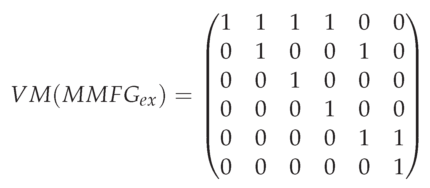
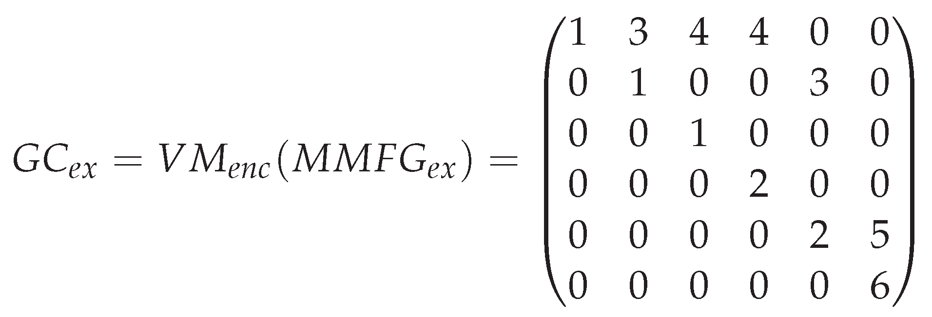
can be ordered according to the corresponding MMFG, e.g., by applying a breadth-first-search, but also other ordering strategies could be applied. As the ordering does not effect the Graph Code algorithms and concepts as such, in the following examples, we chose a manual ordering to maximize illustration. In the Graph Code matrix representation, each node field (in the diagonal) of a Graph Code can now be unambiguously mapped to an entry of its Graph Code Dictionary vector, which can be represented as follows:
d i c t G C = ( f t 1 , , f t n )
Applied to the Graph Code of the previous example, the set of feature vocabulary terms F V T e x 
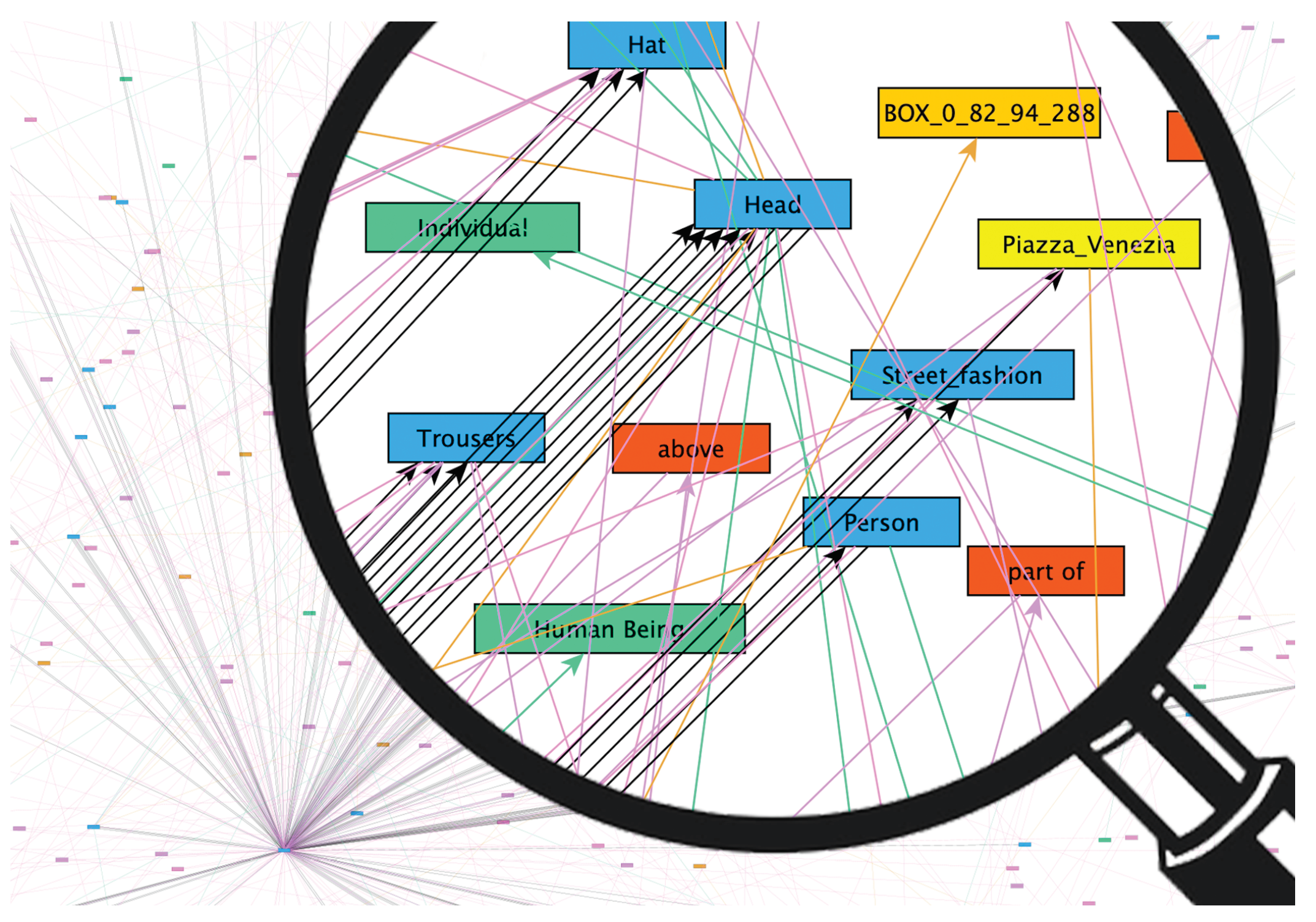
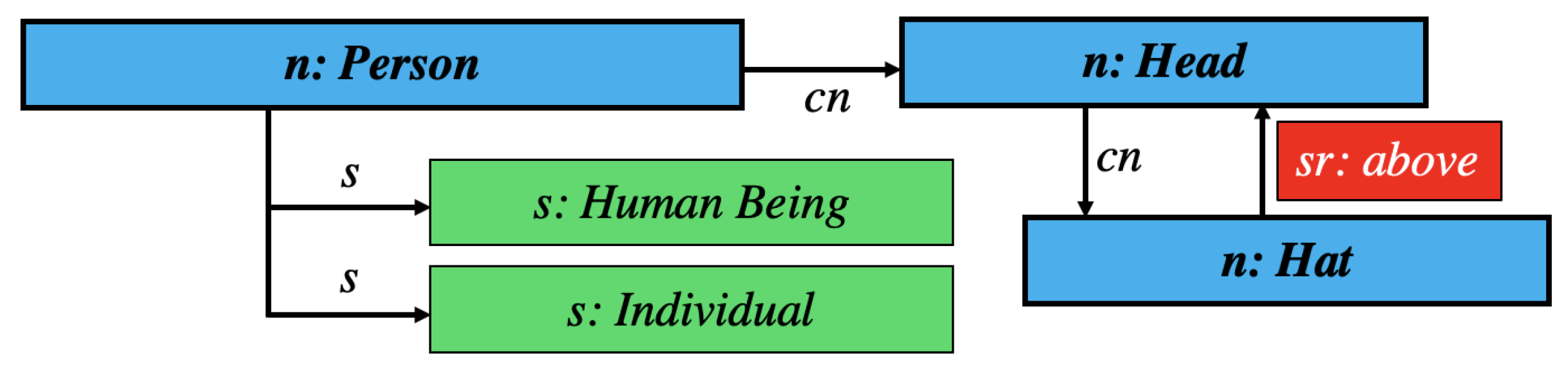
would be {Person, Head, Human Being, Individual, Hat, above}, in which the elements do not have any order. The corresponding vector d i c t e x would be:
d i c t e x = ( P e r s o n , H e a d , H u m a n B e i n g ,
I n d i v i d u a l , H a t , a b o v e )
and—in contrast to the set representation—uniquely identifies each vocabulary term by its position within the vector. Thus, d i c t e x can also be regarded as a indexed list:
Index i123456
f t i PersonHeadHuman BeingIndividualHatabove
When comparing the similarity of two Graph Codes, it is important to compare only feature-equivalent node fields in the diagonal of each matrix to each other. Each Graph Code has its own, individual dictionary-vector d i c t G C , and another Graph Code will have a different dictionary-vector according to the content of its represented MMFG, typically d i c t G C 1 d i c t G C 2 . Feature-equivalent node fields of Graph Codes can be determined through their corresponding Graph Code Dictionaries, as these fields will have positions represented by an equal feature vocabulary term of each corresponding dictionary. For comparison, only the set of intersecting feature vocabulary terms of e.g., two Graph Codes is relevant, as non-intersecting feature vocabulary terms would represent non-common MMFG feature nodes, which cannot be similar. Thus, the set of intersecting feature vocabulary terms F V T 1 , 2 of e.g., two MMFGs can be defined as:
F V T 1 , 2 = { f t 1 , , f t n } = V M M F V G 1 V M M F V G 2
The methodology of intersecting sets can be also applied to Graph Code dictionaries. The intersection of two vectors d i c t 1 , 2 can be defined correspondingly as:
d i c t 1 , 2 = d i c t G C 1 d i c t G C 2
To illustrate the calculation of d i c t 
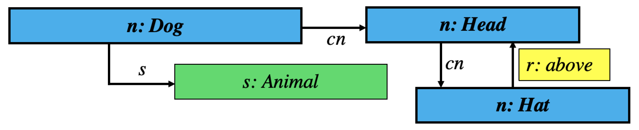
, we introduce a second exemplary Graph Code G C e x 2 based on a M M F G e x 2 as shown in Figure 5 and the corresponding Table 3.
The set F V T e x 2 in this case is above, Dog, Head, Animal, Hat} and the set F T V 1 , 2 of intersecting feature vocabulary terms is above, Head, Hat}. The dictionary-vector d i c t e x 2 thus is:
d i c t e x 2 = ( a b o v e , D o g , H e a d , A n i m a l , H a t )
illustrated as a indexed list, d i c t e x 2 would be:
Index i12345
f t i aboveDogHeadAnimalHat
The vector d i c t e x 1 , 2 represents the dictionary of intersecting vocabulary terms and only contains the subset of vocabulary terms of d i c t e x , where a equal vocabulary term can be found in d i c t e x 2 . The order of intersecting vocabulary terms in d i c t 1 , 2 is given by the order of d i c t e x :
d i c t e x 1 , 2 = ( a b o v e , H e a d , H a t )
From an algorithmic perspective, this means that all elements of d i c t e x are deleted that cannot be found in d i c t e x 2 . Typically, the index position of d i c t 1 , 2 is different from both d i c t 1 and d i c t 2 . For our example, the indexed list representation of d i c t e x 1 , 2 would be:
Index i123
f t i aboveHeadHat
Based on these dictionary-vectors, a translation of equivalent Graph Code positions can be performed, as each feature vocabulary term has a unique position within each of the Graph Code’s dictionaries.
Applications will typically utilize a collection of MMFGs and their corresponding Graph Codes. The overall feature term vocabulary F V T C o l l = { f t 1 , , f t c } containing c vocabulary terms of such a collection of n MMFGs can be defined as the union of all MMFG’s feature term vocabularies and also be represented by the union of all Graph Code Dictionaries d i c t :
F V T C o l l = i = 1 n F V T M M F G i
i , j < n : d i c t = d i c t i × d i c t j
In this d i c t dictionary-union-vector, the ×-operation for calculating the union of dictionary-vectors is implemented by traversing all the collection’s d i c t i dictionaries and collecting unique dictionary vocabulary terms into a single dictionary-vector. In case of our example with d i c t e x and d i c t e x 2 , the calculated d i c t = (Person, Head, Human Being, Individual, Hat, above, Dog, Animal). If a d i c t is calculated for the complete collection of Graph Codes, it can be regarded as a global dictionary-vector with collection-wide unique positions for each feature vocabulary term.
As we will show in the remainder of this paper, an exemplary MMFG could contain about 500 feature nodes and 2000 edges, thus the resulting Graph Code matrix would contain 500 rows and columns and 2500 non-zero entries (500 for the nodes in one diagonal, 2000 for edges between these nodes). Processing many different MMFGs will result in many different Graph Codes having about similar size, but different vocabulary terms, leading to an increase of V C o l l . The Oxford English Dictionary [39] e.g., contains 170,000 English words (Note: translation and multilingual support is not in scope of this paper and does not affect the general concept of Graph Codes). If we assume, that applications exist, which produce English terms as representations for feature-nodes, MMFGs representing the overall vocabulary would result in matrices of size 170,000 × 170,000 resulting in 28.9 billion matrix fields. Calculations on this large number of fields will be no longer efficient enough for MMIR.
Of course, in some use cases, an application-wide dictionary can be required. However, in some other applications, it would be better to apply a much smaller dictionary. Hence, two major approaches of modeling dictionaries can be proposed:
Application-wide dictionary: in this scenario, we assume that any Graph Code will be processed with the dictionary-vector terms d i c t . If in an MMIR application all images are almost similar, a processing and re-processing approach can automatically increase or decrease the collection’s vocabulary terms according to the analysis of new content. All existing Graph Codes have to be adjusted whenever new indexing terms are detected (the size of d i c t increases) or whenever existing multimedia feature content is removed from the collection (the size of d i c t decreases). The key advantage of this approach is, that all Graph Codes have exactly the same size and identical positions represented by their dictionary-vectors. This makes comparisons easier as no further transformation is required. It also simplifies the employment of Machine Learning algorithms. However, a permanent re-processing of all existing Graph Codes can be computationally expensive. In this case, the following scenario should be preferred.
Dictionaries for smaller combinations of individual vocabularies: if images from many different areas (i.e., with many different feature vocabulary terms) have to be processed, two Graph Codes can be compared based on the intersection of their individual Graph Code’s dictionary vectors d i c t . In this case, a mapping of corresponding feature vocabulary terms by their position within each dictionary-vector can be performed and equivalent node matrix fields can be calculated by a simple transformation (i.e., re-ordering) of one of the dictionary-vectors. As this also eliminates lots of unnecessary operations (e.g., comparing unused fields of d i c t ), this approach can be very efficient, when Graph Codes vary a lot within a collection.
Applied to G C e x and G C e x 2 of our above example, the application-wide dictionary d i c t would result Graph Codes with a size of 9 × 9 matrix fields, whereas d i c t would result in a intersection matrix of 3 × 3 fields. This intersection matrix M ( G C ) can be calculated of a G C by removing any rows and columns, that are not part of d i c t . Table 4 shows the intersection matrices of G C e x and G C e x 2 .
For the comparison of these intersection matrices, we would like to apply the standard matrix subtraction. However, due to the different orders of d i c t e x and d i c t e x 2 , the matrix field positions of the matrices do not represent the same feature vocabulary terms. For example, the field (2,1)of G C e x represents the relationship between Hat and Head, but the equivalent relationship in G C e x 2 is located in field (3,2). To solve this, we introduce a equivalence function f e q u ( M ) , which transforms a Graph Code intersection matrix or the corresponding dictionary-vector in a way, that the corresponding dictionary-vector is ordered according to d i c t .
Thus, equivalence of a matrix field ( m i , j ) in M ( G C i ) and a matrix field ( n k , l ) in M ( G C j ) and corresponding dictionary vectors d i c t i and d i c t j can be defined as: ( m i , j ) M ( G C i ) , ( n k , l ) M ( G C j ) :
M ( G C i ) f e q u ( M ( G C j ) )
d i c t i ( i ) = f e q u ( d i c t j ( k ) ) d i c t i ( j ) = f e q u ( d i c t j ( l ) )
In the case of comparing only two Graph Codes, d i c t is automatically ordered according to the first Graph Code. Thus, in this case, the second dictionary-vector would be re-ordered to match the order of the first one. This reordering is applied to the corresponding intersection matrix of the Graph Code. In our example, d i c t e x 2 = ( a b o v e , H e a d , H a t ) would be reordered to match d i c t e x = ( H e a d , H a t , a b o v e ) . Thus, the resulting reordered intersection matrix would be as shown in Table 5.
Based on this description of the representation of MMFGs as on the definition of Graph Code feature vocabularies, we will now define a metric to calculate similarity of Graph Codes as a basis for MMIR retrieval applications.

3.2. Graph Code Similarity

In this section, we define a metric, that enables MMIR application to compare Graph Codes and thus utilize them for retrieval. In case of Graph Codes and their matrix-based representation, the calculation of similarity requires the consideration of rows, columns and fields representing nodes and edges (i.e., node relationships) of a MMFG. These nodes and relationships have to be of equivalent node or relationship type for comparison. This means, that it is important to compare the correct matrix field position to each other, which typically is different in e.g., two Graph Codes. Matrix field positions employed for the definition of a metric represent nodes (i.e., detected features) or edges (i.e., detected node-relationships), edge-types (i.e., detected node relationship types), and their type values. The definition of a metric for Graph Codes has to be applicable for matrices, where rows and columns represent MMFG nodes and the corresponding feature vocabulary terms. Matrix cells represent node types (in one diagonal) and all other non-zero matrix fields represent edge types and their values. Based on these characteristics of Graph Code we can define a metric:
M G C = ( M F , M F R , M R T )
as a triple of metrics containing a feature-metric M F , a feature-relationship-metric M F R and a feature-relationship-type-metric M R T .
The Graph Code Feature Metric
The feature-metric M F can be employed to calculate the similarity of Graph Codes according to the intersecting set of dictionary vocabulary terms. M F is defined as the ratio between the cardinality of d i c t the intersecting dictionary vocabulary terms and the cardinality d i c t i a Graph Code’s dictionary vector. In the following formulas, the notation | v | for vectors denotes the cardinality of a vector v, i.e., the number of elements in this vector:
M F ( G C i , G C j ) = | d i c t | | d i c t i |
Thus, the more features are common in e.g., two MMFGs, the higher the similarity value based on M F - independent of the relationships between these corresponding MMIR features. In case of the example above, the numerical distance between G C e x and G C e x 2 based on the metric M F is:
M F ( G C e x , G C e x 2 ) = | d i c t e x 1 , 2 | | d i c t e x | = 3 6 = 0.5
The Graph Code Feature Relationship Metric
The feature-relationship-metric M F R is the basis for the similarity calculation of MMFG-edges, i.e., the non-diagonal and non-zero fields (representing edges of deliberate types) of the Graph Code’s matrix representation. This metric is only applied to equivalent fields (i.e., relationships with the same source and target node) of intersection matrices M of two Graph Codes. We base this metric on the non-diagonal fields of the Adjacency Matrix A M ( M ) (i.e., the matrix containing only the values 1 and 0). Then, M F R can be defined as ratio between the sum of all non-diagonal fields and the cardinality of all non-diagonal fields. Sum and cardinality of all non-diagonal fields are calculated by subtracting the number of nodes n from the sum or cardinality of all fields:
M F R ( G C i , G C j ) = A M ( M i , j ) n | A M ( M i ) | n
Thus, M F R represents the ratio between the number of non-zero edge-representing matrix fields and the overall number of equivalent and intersecting edge-representing matrix fields of e.g., two Graph Codes. Note, that in this way, the metric M F R counts all edges existing between source and target nodes, independent of the equivalence of the edges’ types.
Applied to our example, the  A M ( M ( G C e x ) ) and the equivalent matrix f e q u ( M ( G C e x 2 ) ) is shown in Table 6 and Table 7.
Looking at the two Graph Codes in Table 6 and Table 7, there are six potential positions representing edges: three fields in the upper right of the diagonal and three fields in the lower left. Out of these possible positions, only two contain edges. These are located in matrix positions (2,1) and (3,2). Thus, only two out of six possible edge representing matrix field positions have a non-zero value. Thus, the numerical distance of the metric M F R :
M F R ( G C e x , G C e x 2 ) = A M ( M i , j ) n | A M ( M i ) n | =
5 3 9 3 = 2 6 = 0.33
Note, that currently only the existence of an edge—independent from its type—is employed for the metric M F R . However, also the type of each relationship can indicate additional similarity. Hence, we will introduce an edge-type-based metric in the next section.
The Graph Code Feature Relationship Type Metric
The metric M R T is based on the feature-relationship-types of Graph Codes. As the Graph Code encoding function f e n c encodes different MMFG edge-types with different base values (see Section 2.4), feature-relationship-type-similarity can only exist, when the edge-types represented by equivalent matrix fields of Graph Codes are equal. In case of M R T , calculations are performed no longer on the adjacency matrices of Graph Codes, but on the M matrices of the Graph Codes (see Table 8).
A matrix field is equal to another, if the subtraction of their values returns zero. If all equivalent fields are equal, the sum of these fields is zero. While M F R is based on the pure existence of a non-zero edge representing matrix field, M R T additionally employs the value of this matrix field (representing the relationship type) and hence represents the ratio between the sum of all non-diagonal matrix fields and their cardinality:
M R T ( G C i , G C j ) = i , j n , i j ( | M i M j | ) | M i | n
In our example, the difference of these two intersection matrices for non-diagonal fields (i.e., i j ) is calculated as:
| M ( G C e x ) M ( G C e x 2 ) | = 0 0 0 0 0 1 0 0 0
Thus, the mathematical sum of this matrix is 1. This means, that one out of six possible fields had a different edge type value. The numerical distance of the metric M R T for these two Graph Codes can be calculated as:
M R T ( G C i , G C j ) = i , j n , i j ( | M i M j | ) | M i | n =
1 9 3 = 1 6 = 0.16
Thus, in terms of our example, the overall similarity M G C between G C e x and G C e x 2 is:
M G C ( G C e x , G C e x 2 ) = ( M F , M F R , M R T ) =
( 0.5 , 0.33 , 0.16 )
This means, that the similarity based on common vocabulary terms M F is 0.5, the similarity based on common edge positions M F R is 0.33, and the similarity of equal edge types M R T is 0.16.
Based on the metrics for Graph Codes, MMIR retrieval can utilize comparison functions to calculate a ranked list of results. In the next and subsequent part, we will illustrate the Graph Code query construction and retrieval execution algorithms.

3.3. Querying with Graph Codes

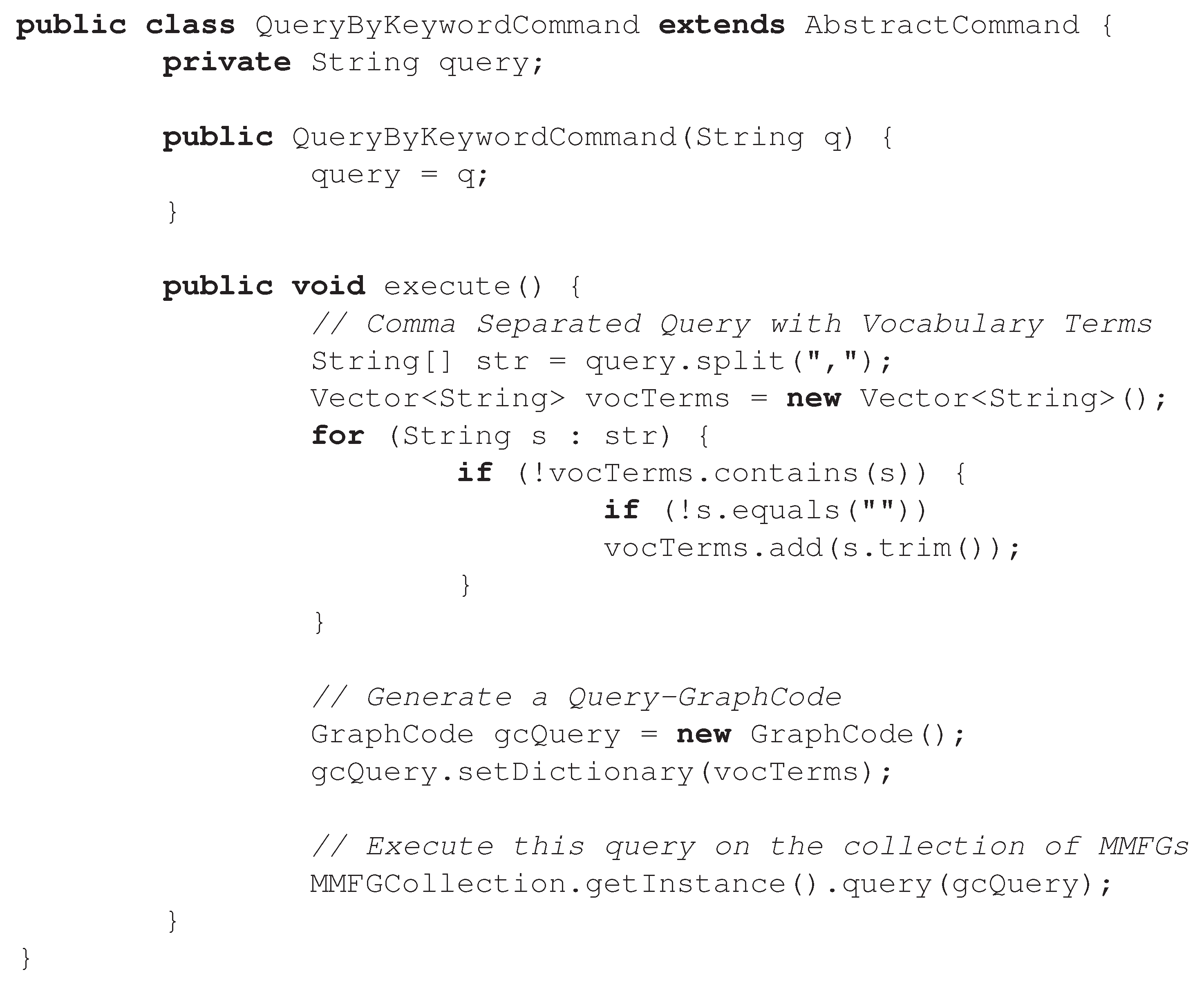
Query Construction based on Graph Codes is possible in three ways: a manual construction of a query Graph Code G C Q u e r y , the application of the Query by Example paradigm, or an adaptation of existing Graph Codes. These three options are described in this section.
A manual construction of a M M F G Q u e r y by users can result in a G C Q u e r y Graph Code, which then is employed for querying. This manual construction could be performed by entering keywords, structured queries (e.g., in a query language like SPARQL [40]), or also natural language based commands [41] into a MMIR application’s query user interface. The  M M F G Q u e r y and corresponding G C Q u e r y in this case is created completely from scratch.
Query construction can be based on the Query by Example paradigm [42]. In this case, a  G C Q u e r y is represented by an already existing Graph Code, which typically is selected by the user to find similar assets in the collection of a MMIR application.
An adaptation of an existing Graph Code can lead to a G C Q u e r y as well. A refinement in terms of Graph Codes means, that e.g., some non-zero fields are set to zero, or that some fields get new values assigned according to the Graph Code encoding function f e n c . From a user’s perspective, this can be performed by selecting detected parts of corresponding assets and choosing, if they should be represented in the query or not.
A prototype for all three options of Graph Code querying is illustrated in [22] and available on GitHub [20]. The adaptation of existing MMFGs in terms of the Graph Code matrices is shown in Table 9, which shows an exemplary G C Q u e r y and an exemplary adapted version G C Q u e r y .
To further optimize the execution of such a query, we construct a compressed Graph Code G C Q u e r y - C by deleting all rows and columns with zero values from an adapted Graph Code. This G C Q u e r y - C provides an excellent basis for comparison algorithms, as it typically contains very few entries. In the previous sections, we showed, that this would also reduce the number of required matrix comparison operations. In our example, G C Q u e r y - C would semantically represent a search for images containing a red watch (see Table 10).
Instead of traversing feature graphs to match sub-graphs, a  G C Q u e r y comparison based on Graph Codes employs matrix-operations to find relevant Graph Codes based on their similarity to the G C Q u e r y implemented by the metric M G C . This approach facilitates the use of Machine Learning, Pattern Matching, and specialized hardware for parallelization of query execution, which is described in more detail in the next section.

3.4. Information Retrieval Based on Graph Codes

In Section 3, we have already introduced the retrieval function:
I R G C ( G C Q u e r y ) = ( G C 1 , , G C n )
which returns a list of Graph Codes ordered by relevance implemented on basis of the similarity metric:
M G C = ( M F , M F R , M R T )
and thus directly represents the retrieval result in form of a ranked list. The calculation of this ranked list can be performed in parallel, if special hardware is available. In many MMIR applications, this calculation can also be done in advance. For a given query Graph Code G C Q u e r y , a similarity calculation with each Graph Code G C of the collection is performed, based on the Graph Code metric M G C . Compared to graph-based operations, matrix-based algorithms can be highly parallelized and optimized. In particular, modern GPUs are designed to perform a large number of independent calculations in parallel [43]. Thus, the comparison of two Graph Codes can be performed in O ( 1 ) on appropriate hardware, which means that the execution of a complete matrix comparison can be fully parallelized and thus be performed in a single processing step. It is notable, that even current smartphones or tablets are produced with specialized hardware for parallel execution and ML tasks like Apple’s A14 bionic chip [
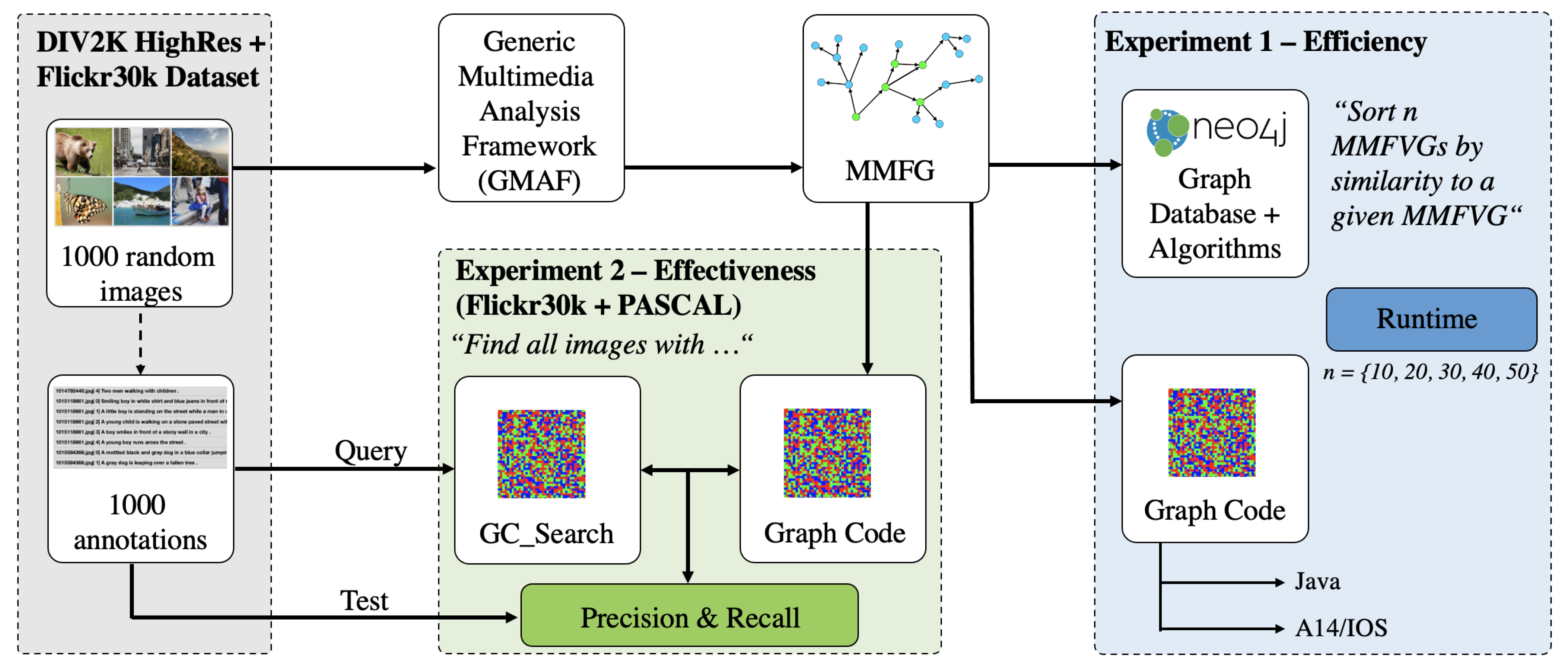
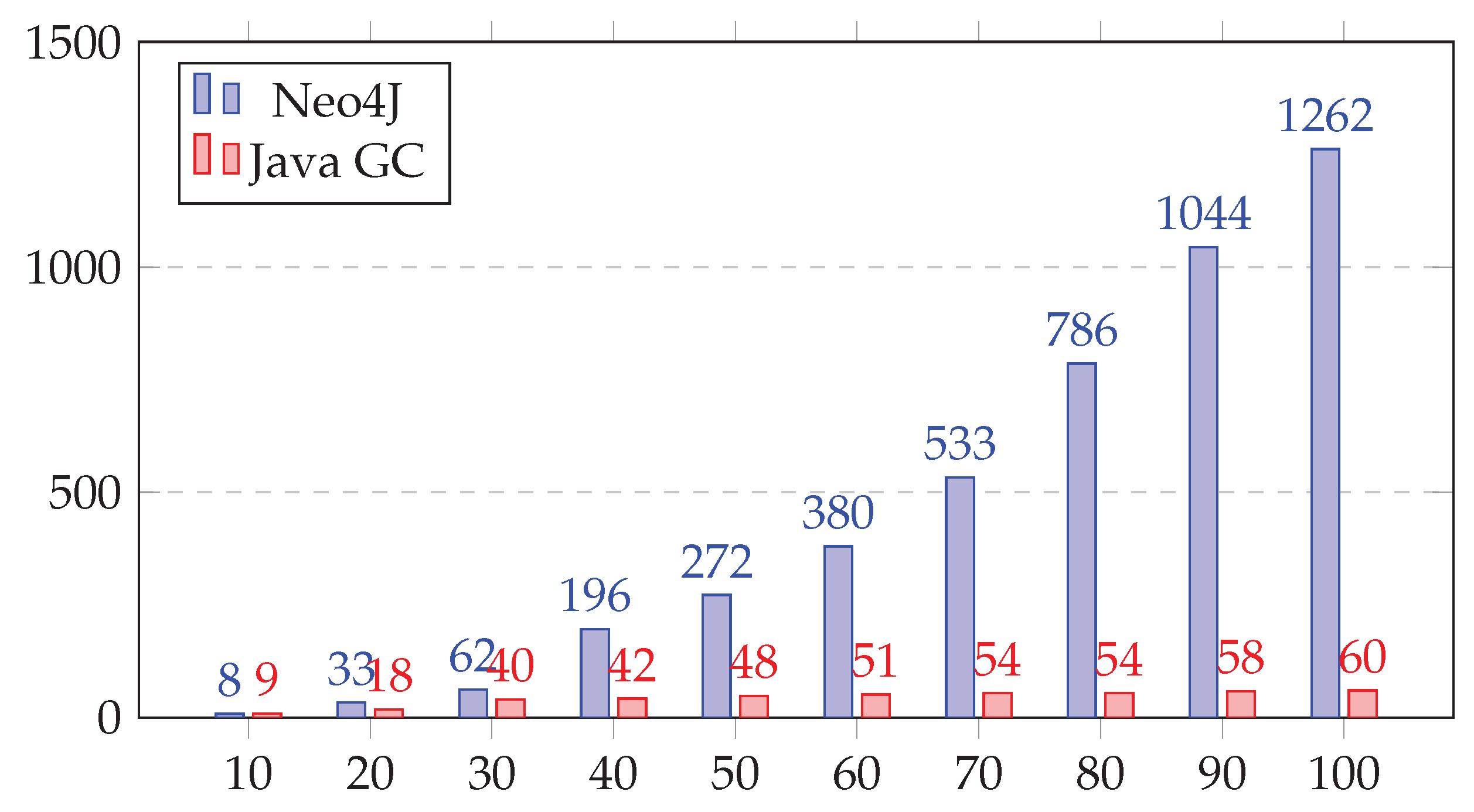
44]. Hence, the Graph Encoding Algorithm performs well also on smartphones or tablets. In the evaluation section of this paper (Section 5), we give detailed facts and figures. The basic algorithm for this comparison and ordering is outlined in pseudocode below:
for each GC in collection
    --- parallelize ---
    calculate the intersection matrices
    of GC_Query and~GC
        --- parallelize each ---
        calculate M_F of GC_Query and GC
        calculate M_FR of GC_Query and GC
        calculate M_RT of GC_Query and GC
        --- end parallelize each ---
    compare
    --- end parallelize~---
    order result list according to
    value of M_F
      value of M_FR where M_F is equal
        value of M_RT where M_F and M_FR are equal
    return result list
To calculate the ranked result list, this algorithm employs the three metrics M F , M F R and M R T in such a way, that first, the similarity according to M F (i.e., equal vocabulary terms) is calculated. For those elements, that have equal vocabulary terms, additionally the similarity value of M F R for similar feature relationships is applied for ordering. For those elements with similar relationships (i.e., edges), we also apply the metric M R T , which compares edge types. So, the final ranked result list for a G C Q u e r y Graph Code is produced by applying all three Graph Code metrics to the collection.

3.5. Discussion

In this section, we presented the conceptual details, their mathematical background and formalization, a conceptual description of the and algorithms for processing Graph Codes and their application for MMIR. We introduced Graph Code feature vocabularies and dictionaries as a foundation for further modeling. Particularly Graph Code dictionary vectors are the basis for several operations and provide a clearly defined, indexed list of vocabulary terms for each Graph Code. The design of MMIR applications can employ application-wide dictionaries or dictionaries for smaller or individual vocabularies, which provides high flexibility in the application design when using Graph Codes.
Hence, we also introduced an example to illustrate the corresponding matrix operations, which is also employed as a basis for the calculation of Graph Code similarity. Similarity of Graph Codes is defined by a metric M G C = ( M F , M F R , M R T ) , which addresses different properties of the underlying MMFG. Firstly, M F provides a measure for similarity based on the vocabulary terms of Graph Codes. Secondly, M F R checks, if equal edge relationships exist between the two Graph Codes and thirdly, M R T compares the relationship type of existing edges. With this metric-triple, a comprehensive comparison of Graph Codes can be implemented. Based on this metric, we discussed the construction of Graph Code queries, which can be performed manually, as Query by Example, or in terms of a adaptation of existing Graph Codes and will result in a query Graph Code. This query object can be compressed and will provide an excellent basis for comparison algorithms based on the metric M G C . We also showed, that MMIR retrieval based on Graph Codes can be highly parallelized.
In general, all these introduced concepts show, that it is possible to perform calculations in a 2D matrix space instead of traversing graph structures and to integrate features of various sources into a single feature graph. However, to demonstrate that these calculations provide the expected advantages compared to graph-based operations, a proof-of-concept implementation and corresponding evaluation is required. Hence, we will now outline the most important facts and show, that by using Graph Codes a significant improvement of efficiency and effectiveness in MMIR applications can be achieved in the following sections of this paper.

4. Implementation and Testing

For the implementation of the presented algorithms and concepts, we chose Java [45] and Swift [46] as programming languages. As our corresponding frameworks like the Generic Multimedia Analysis Framework [19] are already implemented in Java, we also chose Java as a programming language for the Graph Code algorithms and built components according to the modeling and design section of this paper. For the later evaluation, we also implemented the Graph Code Retrieval algorithm in Swift for IOS [46] to evaluate it on an iPad Pro [47], as we wanted to investigate the use of parallelization in terms of the A14 bionic chip [44] in this device. The implementation basically follows the algorithms and functions described in the previous section, so only a few selected examples will be discussed here.

4.1. Selected Implementation Details

The details of the implementation including source code can be found at GitHub [20], where also a Jupyter notebook [48] is available. In addition to this Java implementation, we also built a second implementation based on the graph-database Neo4J [49], which we can use for comparison. Hence, the GMAF has been extended to provide an additional MMFG-export option in the Neo4J format. Thus, in both Neo4J and the Java implementation, the same MMFGs can be used for further processing.
For the implementation of the GMAF, we applied a software design based on the GoF-Patterns for reusable software components [50]. As we chose Java as the programming language for the GMAF prototype, these patterns are aligned with the programming language’s constraints. Figure 6 e.g., shows the source-code of the Query Construction by keywords, which follows the Command Pattern. Each keyword entered by the user is employed to fill the vocabulary terms of a Graph Code and then processed on the MMFGs of the collection.
Another selected example is the calculation of the ranked result list based on Java standards, which is shown in Figure 7. As Java internally uses a so called comparator mechanism to efficiently sort indexed lists (in this case a Vector), we implemented the frameworks to utilize these structures. The Pseudo-Code of Section 3.4 is thus transformed into a Java-complying form, where the logical processing rules of cascaded metrics are represented by a mathematical operation to achieve single values for comparison.
A screenshot of the GMAF prototype is given in Figure 8. This screenshot shows a key-word based query, the ranked result list in the centre of the screenshot and the calculated metric values for each of the MMFGs in the collection. On the right side of the GMAF, the current selected asset and its corresponding Graph Code is visible.

4.2. Hardware and Environment

For the comparison of the Neo4J and the Java implementation, we installed both the Neo4J graph database and the Java Graph Code algorithms on a 16 inch MacBook Pro (2.4 GHz, 8-Core Intel Core i9 processor, 64 GB RAM, AMD Radeon Pro 5500M 4 GB Graphics card, 2 TB SSD Storage) running MacOS 11.2 Big Sur. For comparison reasons, we also installed Windows 10 on this machine and double-checked, that the evaluation results, described in the next section, are equal—independent of the operating system. For further comparisons, we also implemented the Graph Code algorithms in Swift for IOS and ran them on an iPad Pro (13 inch, 4th generation, A14 bionic ML chip). In addition to running the Graph Code natively on the iPad, we also ran the algorithm in the iPad Simulator on the MacBook Pro.

4.3. Level of Detail

The basis for our experiments are Graph Codes, which can be generated with different Levels Of Detail (LOD) [22]. In our evaluation, this generation is performed by the GMAF framework [19] (see also Figure 8), which provides options to determine the number of recursions used for object detection. Recursions in GMAF mean that a detected object’s bounding box was processed again and the identified sub-objects were fused into the resulting MMFG. After some recursions, the bounding boxes became to small to represent any useful detected object and the GMAF processing terminates for this object. The higher an image’s resolution, the more recursions were possible and the higher the LOD of the detected features. To illustrate the improvement in quality, when using Graph Codes and the GMAF framework, we evaluated a given high-resolution image (see Figure 9) and applied the GMAF processing with different settings for the LOD.
Table 11 shows the results of this testing. Additionally, a selection of the detected feature vocabulary terms F V T M M F G for each recursion is also given in the table for exemplary purposes. These results were generated only by applying object detection, no additional meta-data were attached to the MMFGs, which would further increase the number of nodes and edges. This means, that all the vocabulary terms shown in Table 11 have been actually detected by the GMAF framework.
This testing showed that the LOD could be increased, if the source image was of high resolution. Based on this prerequisite, we focus on a detailed evaluation of our prototypical proof-of-concept implementation in the remainder of this paper.

5. Evaluation

To evaluate the performance of our proof-of-concept implementation, we followed well established methods for experiments to address efficiency (i.e., runtime behavior of the MMIR application) and effectiveness (precision and recall). To validate our assumptions with respect to modeling and implementation, we performed several experiments with different constraints. An overview of the experiments is given in Figure 10. Input data were taken from the DIV2K and Flickr30k datasets. Experiment 1 evaluated the efficiency of the algorithms based on the number of input graphs n. Experiment 2 evaluated the effectiveness of the Graph Code Algorithm based on annotations from the Flickr30k dataset. In Experiment 1, we addressed efficiency (i.e., runtime behavior) of our Java implementation compared to a Neo4J implementation of MMFGs. To demonstrate the performance for different sample data, we executed this experiment with three available sample datasets, the Flickr30k dataset, the DIV2K dataset and a high-resolution sample image. In Experiment 2, we investigated effectiveness based on the available annotated sample datasets Flickr30k and DIV2K. During the Flickr30k experiment, we discovered some flaws in the annotations of this dataset and thus split the experiment into a sub-experiment which did not regard synonyms, and another sub-experiment which also took synonyms into account. These experiments are discussed in the following sections.
As discussed in our implementation section (Section 4), the LOD is very important for MMIR applications. However, existing datasets do not meet the requirements of a full level-of-detail processing. The Flickr30k dataset contains only low-resolution images, which limits number of recursions and therefore the LOG in object-detection to level 2, as then no further objects can be identified due to the low resolution of the sample images. The DIV2K dataset provides higher resolutions, and can be employed up to a LOD of level 3, but to measure full feature detection capabilities of the GMAF, an annotated dataset of high-resolution images would have to be created and maintained. Currently, such a dataset is not yet existing. We are considering creating and publishing such a dataset in our future work.
Fortunately, for proving efficiency and effectiveness of Graph Codes, the LOD achieved with current datasets was high enough to employ existing annotated datasets for our experiments. In the following sections, we will discuss these experiments in detail.

5.1. Experiment 1—Efficiency

The goal of this initial efficiency experiment is to compare the Graph Encoding Algorithm to standard graph algorithms. Our hypothesis was that Graph Codes performed better than graph traversal-based algorithms. For retrieval, the calculation of similarity is very important. Thus, we compared the retrieval algorithm of Neo4J (Node similarity) to the Graph Encoding Algorithm performed on the same machine (Java implementation) and on Apple’s A14 Bionic in an iPad Pro. As input for the similarity calculation we used a selection of c random images of the corresponding dataset and calculated the overall number of nodes n and edges e. To show the correspondence between the size of the MMFG, and the runtime behavior, we performed this experiment on existing datasets with low (Flickr30K), medium (DIV2K) resolution samples, and on a high-resolution image downloaded from Adobe Stock [51]. For the low resolution evaluation with the Flickr30k dataset, we were able to produce a LOD of level 3. The results of this experiment are shown in Table 12 and Figure 11. The medium resolution evaluation with the DIV2K dataset produced LODs of level 4 and 5 (see results in Table 13). The high-resolution evaluation generated a LOD of level 6 with results summarized in Table 14. This last evaluation has also been performed on an Apple iPad Pro and on a MacBook Pro (IOS Simulator).
For all these experiments, we performed the standard similarity search (production quality) of Neo4J according to the Neo4J guidelines and benchmarks [49]. Before each experiment, we cleared the Neo4J database and loaded only the nodes, that were relevant for the experiment. In the Neo4J query, we adjusted the number of recursions for the graph-search to the LOD-level of the MMFG. The following query was applied to each set (exemplary with p = 4 ):
MATCH (r1:Node {name: ’N_Root_Image_Search’}
    )-[*..4]->(child1)
    WITH r1, collect(id(child1)) AS r1Child
        MATCH (i:Image)-[:img]->
        (r2:Node {name: ’N_Root_Image’}
    )-[*..4]->(child2)
 
    WHERE r1 <> r2
        WITH r1, r1Child, r2, collect(id(child2))
        AS~r2Child
    RETURN r1.image AS from, r2.image AS to,
        gds.alpha.similarity.jaccard
        (r1Child, r2Child)
    AS similarity
Experiment 2 in Table 14 showed that the best performance was achieved with the iPad Pro application running in Apple’s Simulator application. The reason for this is, that in this case they ran natively on a Apple MacBook Pro with 64 GB of memory and 8-core-CPU, which was still faster than any mobile device. It was remarkable though, that the native performance on the iPad Pro was still better than any other measuring (e.g., Neo4J or Java).
In discussion of Experiment 1, we can state that the Graph Code algorithms outperformed current graph traversal algorithms by more than a factor of five and, more importantly, grew linearly, in contrast to the exponential growth of graph traversal-based algorithms. The larger the graph got and the more levels it contained, the larger the difference was between classic graph traversal algorithms and the Graph Code processing. This did not only apply to graphs stored in graph-databases like Neo4J, it also applied to graph traversal based algorithms like stated in Section 2 or [31], as all these algorithms grew exponentially. Our experiments show, that Graph Code algorithms remained linear independent from the scale of the corresponding MMIR collection. These results validate our hypothesis, that Graph Codes are more effective than current graph-based algorithms for MMIR. Of course, there are many options also within Neo4J to tune and optimize the database and the algorithms, but in any case, graph traversal has square or exponential complexity, whilst Graph Codes performed linearly. Additionally, for Graph Codes several optimizations according to the MMIR application design are possible and will be addressed in our future work. Another important point for multimedia processing is that Graph Codes performed very well on smartphones or tablets (see Table 15) as they could utilize the existing GPU hardware of these devices. Therefore, the conclusion of experiment 1 is that any multimedia application can employ fast indexing and retrieval directly on the user’s device. However, further experiments with different datasets and benchmarks have to be conducted, to evaluate the performance of Graph Codes in various application areas.

5.2. Experiment 2—Effectiveness

To determine the effectiveness of the Graph Code Algorithm, we selected five test-queries from the annotations of our random set of 1000 Flickr30k images and calculated values for precision and recall for these. Our hypothesis was that precision and recall values should increase due to the higher LOD. For this experiment, we did not feed any metadata into the GMAF, which would be the case normally. So, the results reflect the pure object detection capabilities of the GMAF-framework without any semantic enrichment. Indexing and retrieval was done using Graph Codes. However, as the Flickr30K dataset was annotated manually, lots of different terms were used to describe the same objects as no common ontology was applied. Hence, we had to perform two sub-experiments to reflect these flaws in standardization of the dataset. In the first experiment (No-Synonym Experiment), only the nouns from the queries were used to create a G C S e a r c h object. This experiment delivered results for “guitar” only, when the processing of the image detected the term “guitar”. The second experiment (With-Synonym Experiment) also employed synonyms for the nouns as well when creating the G C S e a r c h . In this case, the G C S e a r c h would contain also synonyms in the query. So when querying “guitar”, it would contain e.g., “banjo” or “bass” in the query as well.
Thus, these experiments also reflect the quality of standardization within the Flickr30K dataset. Table 16 and Table 17 show values for the relevant objects r e l in the dataset, the selection s e l by the algorithm, the number of true positive results t p , the number of true negative results t n , precision P and recall R. Results are also shown in Figure 12.
For discussion of the results, we further investigated the values of P and R and discovered some flaws in the Flickr30k dataset, as in our manual review of the annotations and corresponding images, we found lots of inaccurate annotations. Approximately 80% of the “false negatives” e.g., have been actually correct, but the annotations of the input images were wrong. In general, the Flickr30k dataset would have to be reviewed and corrected in order to perform further tests.
After discovering these flaws in the Flickr30k dataset, an additional experiment with the PASCAL VOC dataset [38] was performed. This dataset comes with predefined object classes and annotations. An experiment of R. Scherer [52], published 2020 and proposing a “Salient Object Detector and Descriptor by Edge Crawler” algorithm produced an average precision of 78.58%. Results of our experiment are shown in Table 14 and Figure 13 and show, that the GMAF and Graph Code processing increased the average precision to 96.26%.
In discussion of this experiment, it can be stated, that the object detection of GMAF and the corresponding Graph Code representation actually was much more accurate than the metadata of the annotation files of the Flickr30k dataset. In “real world” tests, we were able to produce Precision and Recall results of more than 97%. The experiment with the PASCAL dataset proved this as well and provided about 15% better results with an average precision of 96% and a recall of 92%. These results validate our hypothesis, that the Graph Codes significantly increased the effectiveness of MMIR due to their higher LOD. Thus, we can conclude, that the accuracy of the results in MMIR applications was even higher than any manual annotation as the GMAF fuses detected objects with textual annotations found in social media posts, metadata, or on corresponding websites.
Summarizing this section, our modeling and implementation has been validated by showing, that the actual results in respect of efficiency and effectiveness were better than current reference algorithms and that thus Graph Codes are highly relevant for future MMIR applications. The final section of this paper provides an overall conclusion and outlook to future work.

6. Conclusions and Outlook

In this paper, we discussed the mathematical model of Graph Codes and the advantages of matrix calculations compared to graph traversal operations for Graph Codes, by ensuring that Graph Codes can be regarded semantically equivalent. We were able to demonstrate, that Graph Codes provide a fast and easy-to-implement solution for MMIR applications, which utilizes feature graph structures. Our experiments show, that calculations in the 2D matrix space significantly outperform graph traversal algorithms and that the implementation of Graph Codes can be ported to any device (e.g., tablets or smartphones) without significant hurdles. Graph Codes do not require any databases or other prerequisites and can be executed directly within any application. This facilitates installation and deployment of Graph Code based applications.
We also discovered some open remaining challenges. In this paper, we have focused on images, but it has to be mentioned, that all these concepts apply similarly to other multimedia types, e.g., video, text, or audio. The only difference is, that for other multimedia types, some other prerequisites must be considered. As an outlook to future work, these are shortly summarized here:
  • Video: a video is a collection of images, which are typically represented by key-frames of the video. In terms of MMFG and Graph Code processing, we represent a single video as a sub-collection, for which an unioning Graph Code based on F T V S u b C o l l is generated. In this F T V S u b C o l l , any feature from any image of the video is contained. When the retrieval algorithm identifies this video (i.e., a collection of images) as a result, a further processing of each single Graph Code of the sub-collection produces the exact key-frames, which are valid retrieval results. In case of video, each MMFG of this sub-collection also contains time code-information, i.e., the exact temporal position of the feature within the video.
  • Text: similar to video, we also regard text documents as a sub-collection of MMFGs. In case of large documents, this sub-collection can contain sub-collections itself and thus represent a document’s structure, i.e., chapters, sections, subsections, sentences. The level of sub-collections depends on the structure of the documents in the MMIR application. Retrieval is then executed similarly to the retrieval of video feature information.
  • Audio: for audio processing, we apply NLP algorithms as illustrated in [41], which produce a textual representation of spoken words. This textual representation can be processed similar to documents in terms of MMFGs and Graph Codes.
  • Multimedia: in many cases, the described media types are a fused. A video, e.g., contains not only key-frames, to which object detection can be applied. It also contains audio layers with spoken words, textual on-screen information (like news tickers), which provide additional scene-related information, written metadata in, e.g., the video’s MPEG7 description [17], and Social Media posts related to this video in form of other texts and images. Figure 14 illustrates a typical example.
Further research on these topics remain to be conducted. When features of various multimedia types are fused into a single MMFG, this would lead to an increase of the LOD in the MMFGs. Another major challenge is, that a well annotated set of sample data for high-resolution, feature-rich MMIR applications has to be created. Our future work will address these challenges to validate further, that Graph Codes provide an efficient extension to multimedia databases for indexing and retrieval.

Author Contributions

Conceptualization and methodology: S.W. and M.H.; software, validation, formal analysis, investigation, resources, data curation, writing: S.W.; review, editing and supervision: B.V., P.M.K. and M.H. All authors have read and agreed to the published version of the manuscript.

Funding

This research received no external funding.

Institutional Review Board Statement

Not applicable.

Informed Consent Statement

Not applicable.

Data Availability Statement

The data presented in this study are openly available in [20].

Conflicts of Interest

The authors declare no conflict of interest.

References

  1. Spyrou, E. Semantic Multimedia Analysis and Processing; CRC Press: Boca Raton, FL, USA, 2017; ISBN 978-1-351-83183-3. [Google Scholar]
  2. Clement, J. Social Media—Statistics & Facts. 2020. Available online: https://www.statista.com/topics/1164/social-networks/ (accessed on 23 August 2020).
  3. W3C.org. W3C Semantic Web Activity. 2020. Available online: http://w3.org/2001/sw (accessed on 23 August 2020).
  4. Neo4J Inc. Neo4J. 2020. Available online: https://neo4j.com/top-ten-reasons/ (accessed on 24 November 2020).
  5. CXL.com. Reduce Your Server Response Time for Happy Users, Higher Rankings. 2021. Available online: https://cxl.com/blog/server-response-time/ (accessed on 13 January 2021).
  6. Beyerer, C. Pattern Recognition—Introduction; Walter de Gruyter GmbH & Co KG: Berlin, Germany, 2017; ISBN 978-3-110-53794-9. [Google Scholar]
  7. Kurland, O. Fusion in Information Retrieval: SIGIR 2018 Half-Day Tutorial. 2018. Available online: https://doi.org/10.1145/3209978.3210186 (accessed on 14 March 2021).
  8. Buhte, A.; Meshram, B.; Harsha, B. Multimedia Indexing and Retrieval Techniques: A Review. Int. J. Comput. Appl. 2012, 35–42. [Google Scholar] [CrossRef]
  9. Subrahmanian, V. Principles of Multimedia Database Systems; Morgan Kaufmann Publishers: San Francisco, CA, USA, 1998; ISBN 978-1-558-60466-7. [Google Scholar]
  10. Leveling, J. Interpretation of Coordinations. 2013. Available online: https://doi.org/10.1145/2484028.2484115 (accessed on 17 May 2021).
  11. Lew, M. Content-Based Multimedia Information Retrieval: State of the Art and Challenges. 2006. Available online: https://doi.org/10.1145/1126004.1126005 (accessed on 17 May 2021).
  12. Hernandez, C. Data Fusion and Label Weighting for Image Retrieval Based on Spatio-Conceptual Information. 2010. Available online: https://dl.acm.org/doi/10.5555/1937055.1937072 (accessed on 23 August 2020).
  13. MIT—Massachutsetts Institute of Technology. Description of Exif File Format. 2020. Available online: http://media.mit.edu/pia/Research/deepview/exif.html (accessed on 23 August 2020).
  14. Dufour, R. Local and Global Models for Spontaneous Speech Segment Detection and Characterization. In Proceedings of the 2009 IEEE Workshop on Automatic Speech Recognition & Understanding, Moreno, Italy, 13 November—17 December 2009; pp. 558–561. [Google Scholar]
  15. FFMpeg.org. Ffmpeg Documentation. 2020. Available online: http://ffmpeg.org (accessed on 23 August 2020).
  16. Mu. Content-Based Video Retrieval: Does Video’s Semantic Visual Feature Matter? 2006. Available online: https://doi.org/10.1145/1148170.1148314 (accessed on 17 May 2021).
  17. Chang, S.-F. Overview of the MPEG-7 standard. IEEE Trans. Circuits Syst. Video Technol. 2001, 11, 688–695. [Google Scholar] [CrossRef]
  18. Jean-Baptiste, A.; Recasens, A.; Schneider, R.; Arandjelovic, R.; Ramapuram, J.; De Fauw, J.; Smaira, L.; Dieleman, S.; Zisserman, A. Self-supervised multimodal versatile networks. arXiv 2020, arXiv:2006.16228. [Google Scholar]
  19. Wagenpfeil, S. GMAF Prototype. 2020. Available online: http://diss.step2e.de:8080/GMAFWeb/ (accessed on 23 August 2020).
  20. Wagenpfeil, S. Github Repository of GMAF and MMFVG. 2020. Available online: https://github.com/stefanwagenpfeil/GMAF/ (accessed on 25 September 2020).
  21. Wagenpfeil, S.; Hemmje, M. Towards AI-bases semantic multimedia indexing and retrieval for social media on smartphones. In Proceedings of the 2020 15th International Workshop on Semantic and Social Media Adaptation and Personalization, Zakynthos, Greece, 29–30 October 2020. [Google Scholar]
  22. Wagenpfeil, S. AI-Based Semantic Multimedia Indexing and Retrieval for Social Media on Smartphones. 2021. Available online: https://www.mdpi.com/2078-2489/12/1/43 (accessed on 17 May 2021).
  23. Gurski, F.; Komander, D.; Rehs, C. On Characterizations for Subclasses of Directed Co-Graphs. 2019. Available online: http://arxiv.org/abs/1907.00801 (accessed on 17 May 2021).
  24. yWorks GmbH. yEd Graph Editor. 2020. Available online: https://www.yworks.com/products/yed (accessed on 23 August 2020).
  25. Fischer, G. Lineare Algebra; Springer Publishing: Heidelberg, Germany, 2014; ISBN 978-3-658-03945-5. [Google Scholar]
  26. Mathworld, W. Adjacency Matrix. 2021. Available online: https://mathworld.wolfram.com/AdjacencyMatrix.html (accessed on 12 March 2021).
  27. Mathworld, W. Eigenvalue Method. 2021. Available online: https://mathworld.wolfram.com/Eigenvalue.html (accessed on 14 February 2021).
  28. Yuan. Graph Similarity Search on Large Uncertain Graph Databases. 2015. Available online: https://doi.org/10.1007/s00778-014-0373-y (accessed on 17 May 2021).
  29. Needham, M. Graph Algorithms; O’Reilly UK Ltd.: London, UK, 2019; ISBN 978-1-492-05781-9. Available online: https://neo4j.com/graph-algorithms-book/ (accessed on 22 July 2021).
  30. Qiu, J.; Dong, Y.; Ma, H.; Li, J.; Wang, K.; Tang, J. Network Embedding as Matrix Factorization: Unifying DeepWalk. 2017. Available online: http://arxiv.org/abs/1710.02971 (accessed on 17 May 2021).
  31. Jeff, J.; Douze, M.; Jegou, H. Billion-scale similarity search with gpus. IEEE Trans. Big Data 2019, 7, 535–547. [Google Scholar]
  32. Text Retrieval Conference. Datasets. 2020. Available online: https://trec.nist.gov/data.html (accessed on 17 May 2021).
  33. Towards Data Science. Over 1.5 TBs of Labeled Audio Datasets. 2018. Available online: https://towardsdatascience.com/a-data-lakes-worth-of-audio-datasets-b45b88cd4ad (accessed on 13 November 2018).
  34. Google.com. A Large and Diverse Labeled Video Dataset for Video Understanding Research. 2021. Available online: http://research.google.com/youtube8m/ (accessed on 5 January 2021).
  35. Young, P. From Image Descriptions to Visual Denotations: New Similarity Metrics for Semantic Inference over Event Descriptions. 2016. Available online: http://shannon.cs.illinois.edu/DenotationGraph/ (accessed on 14 January 2021).
  36. Agustsson, E. NTIRE 2017 Challenge on Single Image Super-Resolution: Dataset and Study. 2017. Available online: http://www.vision.ee.ethz.ch/timofter/publications/Agustsson-CVPRW-2017.pdf (accessed on 17 May 2021).
  37. Grubinger, M. The IAPR TC12 Benchmark: A New Evaluation Resource for Visual Information Systems. In Proceedings of the International Workshop Ontoimage, Genoa, Italy, 22 May 2006. [Google Scholar]
  38. Everingham, M. The PASCAL Visual Object Classes (VOC) Challenge. Int. J. Comput. Vis. 2010, 88, 303–338. [Google Scholar] [CrossRef] [Green Version]
  39. Wikipedia. List of Dictionaries by Number of Words. 2020. Available online: https://en.wikipedia.org/wiki/List_of_dictionaries_by_number_of_words (accessed on 13 December 2020).
  40. W3C.org. SPARQL Query Language for RDF. 2013. Available online: https://www.w3.org/TR/sparql11-overview/ (accessed on 23 August 2020).
  41. Jung. Automated Conversion from Natural Language Query to SPARQL Query. 2020. Available online: https://doi.org/10.1007/s10844-019-00589-2 (accessed on 17 May 2021).
  42. Schmitt, I.; Schulz, N.; Herstel, T. WS-QBE: A QBE-Like Query Language for Complex Multimedia Queries. In Proceedings of the 11th International Multimedia Modelling Conference, Melbourne, Australia, 12–14 January 2005. [Google Scholar]
  43. Nvidia.com. RTX 2080. 2020. Available online: https://www.nvidia.com/de-de/geforce/graphics-cards/rtx-2080/ (accessed on 10 November 2020).
  44. Wikipedia. Apple A14 Bionic. 2020. Available online: https://en.wikipedia.org/wiki/Apple_A14 (accessed on 28 October 2020).
  45. Oracle.com. Java Enterprise Edition. 2020. Available online: https://www.oracle.com/de/java/technologies/java-ee-glance.html (accessed on 23 August 2020).
  46. Apple.com. Apple Development Programme. 2020. Available online: http://developer.apple.com (accessed on 21 November 2020).
  47. Apple. Apple IPad Pro. 2020. Available online: https://www.apple.com/ipad-pro/ (accessed on 27 October 2020).
  48. Jupyter.org. The Jupyter Notebook. 2020. Available online: https://jupyter.org (accessed on 27 October 2020).
  49. Neo4J Inc. Neo4J Graph Database System. 2020. Available online: https://neo4j.com (accessed on 14 December 2020).
  50. Gamma, E.; Helm, R.; Johnson, R.; Vlissides, J. Design Patterns—Elements of Reusable Object Oriented Software; Addison Wesley: New York, NY, USA, 1994; ISBN 0-201-63361-2. [Google Scholar]
  51. Adobe.com. Adobe Stock. 2020. Available online: https://stock.adobe.com (accessed on 2 October 2020).
  52. Scherer, R. Computer Vision Methods for Fast Image Classification and Retrieval; Springer: Berlin/Heidelberg, Germany, 2020; pp. 53–55. ISBN 978-3-030-12194-5. [Google Scholar]
Figure 1. Snippet of the Multimedia Feature Graph (MMFG) of one exemplary asset after exporting it to GraphML (yEd [24] visualization).
Bdcc 05 00033 g001
Figure 2. Excerpt of Figure 1 used as an example-graph M M F G e x .
Bdcc 05 00033 g002
Figure 3. Valuation Matrix V M of M M F G e x . Nodes and existing relationships are represented by a non-zero value.
Bdcc 05 00033 g003
Figure 4. The Graph Code G C e x of M M F G e x represented by the encoded Valuation Matrix V M e n c of M M F G e x .
Bdcc 05 00033 g004
Figure 5. Example instance graph M M F G e x 2 based on the MMFG structure.
Bdcc 05 00033 g005
Figure 6. Code snipped for querying by keywords.
Bdcc 05 00033 g006
Figure 7. Java implementation of the ranked list retrieval.
Bdcc 05 00033 g007
Figure 8. GMAF framework —screenshot.
Bdcc 05 00033 g008
Figure 9. Initial testing —high-resolution image.
Bdcc 05 00033 g009
Figure 10. Experimental setup.
Bdcc 05 00033 g010
Figure 11. Experiment 1—runtime comparison based on the Flickr30K dataset (see Table 12).
Bdcc 05 00033 g011
Figure 12. Experiment 2—true positives are painted in blue, false positives in cyan. See Table 16.
Bdcc 05 00033 g012
Figure 13. Experiment 2—Efficiency of the PASCAL dataset (see Table 14).
Bdcc 05 00033 g013
Figure 14. Visualisation of a typical news-related video screen containing multiple different media types.
Bdcc 05 00033 g014
Table 1. Tabular representation of G C e x = V M ( M M F G e x ) including row and column descriptors, see Figure 2.
PersonHeadHuman BeingIndividualHatAbove
Person111100
Head010010
Human Being001000
Individual000100
Hat000011
above000001
Table 2. Table representation of G C e x including row and column descriptors of Figure 2.
PersonHeadHuman BeingIndividualHatAbove
Person134400
Head010030
Human Being001000
Individual000200
Hat000025
above000006
Table 3. Representation of G C e x 2 including row and column descriptors.
AboveDogHeadAnimalHat
above50000
Dog01340
Head00103
Animal00020
Hat60001
Table 4. Intersection matrices of G C e x and G C e x 2 .
M ( GC ex ) HeadHatAbove M ( GC ex 2 ) AboveHeadHat
Head130above500
Hat025Head013
above006Hat601
Table 5. Reordered and equivalent intersection matrix of G C e x .
f equ ( M ( GC ex 2 ) ) HeadHatAbove
Head130
Hat016
above005
Table 6. Calculation of M F R based on adjacency matrices.
AM ( M ( GC ex ) ) HeadHatAbove
Head110
Hat011
above001
Table 7. Calculation of M F R based on adjacency matrices.
AM ( f equ ( M ( GC ex 2 ) ) ) HeadHatAbove
Head110
Hat011
above001
Table 8. Calculation of M R T based on Graph Code matrices.
M ( GC ex ) HeadHatAbove f equ ( M ( GC ex 2 ) ) HeadHatAbove
Head130Head130
Hat025Hat016
above006above005
Table 9. Exemplary query adaptation based on Graph Codes.
GC Query PersonJimWatchRed GC Query PersonJimWatchRed
Person1351Person0000
Jim0200Jim0000
Watch0011Watch0011
red0001red0001
Table 10. The compressed G C Q u e r y - C Graph Code.
GC Query - C WatchRed
Watch11
red01
Table 11. Initial testing—GMAF processing and LOD.
LOD neSelected FVT MMFG Example Terms
053204Person, Travel, Piazza Venezia, Joy
171274Pants, Top, Pocket, Street fashion
2119475Camera, Bermuda Shorts, Shoe
3192789Sun Hat, Fashion accessory, Watch, Bergen County (Logo)
4228956Mouth, Lip, Eyebrow, Pocket, Maroon
52741189Leather, Grey, Single-lens reflex camera
Table 12. Experiment 1—Flickr30K dataset.
cne N ( p = 3 ) Java
1032615918 ms9 ms
20634321833 ms18 ms
30885484362 ms40 ms
4011005140196 ms42 ms
5013847512272 ms48 ms
6015219979380 ms51 ms
7017921231533 ms54 ms
8019861482786 ms54 ms
90220817051044 ms58 ms
100247918231262 ms60 ms
Table 13. Experiment 1—DIV2K dataset.
cne N ( p = 4 ) N ( p = 5 ) Java iPad
10558327365 ms1027 ms10 ms10 ms
208705420430 ms4688 ms18 ms12 ms
30111977991686 ms44,217 ms26 ms14 ms
40141510,5013303 ms63,705 ms35 ms15 ms
50169212,9943495 ms75,845 ms39 ms15 ms
60202316,0784643 ms-39 ms18 ms
70242719,776--39 ms17 ms
Table 14. Experiment 2—Precision and Recall values for the PASCAL dataset. Average Precision is 96.26%, average Recall 92%.
Class rel sel tp tn PR
bicycle276278265131.000.96
bus17716015730.900.88
car57613535288252.340.91
cat38738437860.990.97
cow20717917810.860.85
dog369378353251.020.95
horse24824223750.970.95
motorbike23922522320.940.93
person733713674390.970.91
sheep25121821350.860.84
Table 15. Experiment 1—high-resolution image, n = 907 , e = 8346 , c = 10 .
AlgorithmRuntime
Neo4J (p = 4)2836 ms
Neo4J (p = 5)54,487 ms
Java GC134 ms
iPad Pro (Simulator)11 ms
iPad Pro36 ms
Table 16. No-Synonym Experiment.
Query rel sel tp tn PR
(A) “Dog”20619018820.980.91
(B) “Man”461204119850.530.25
(C) “Golf”117520.710.45
(D) “Guitar”193017130.560.89
(E) “Bicycle”577854240.690.94
Table 17. With-Synonym Experiment.
Query rel sel tp tn PR
(A) “Dog”20619018820.980.91
(B) “Man”6293982941040.760.47
(C) “Golf”117520.710.45
(D) “Guitar”36302460.800.66
(E) “Bicycle”667960190.750.90
Publisher’s Note: MDPI stays neutral with regard to jurisdictional claims in published maps and institutional affiliations.

