1. Introduction
System-level requirements within aviation are growing increasingly complex due to more stringent restrictions on noise and emissions. With an increasing understanding of the complexities of the environmental impact, the connection between component performance and system-level performance will be of more importance to minimize the risk of sub-optimizing when designing components for next-generation aero engines. The development program of a new turbofan engine generally starts with an initial conceptual design phase involving the optimization of low-fidelity low-order system-level models against system-level objectives and requirements. The initial conceptual design optimization phase defines the architecture concerning the fan stage. It sets ballpark target values for component performance parameters such as the fan pressure ratio, stage efficiency, mass flow per unit area at the inlet and the outlet, and the rotor relative tip Mach number. The conceptual design phase is then followed by the preliminary component design using higher-order modeling techniques to evaluate the feasibility of the targets set by the previous conceptual analysis. Depending on the outcome of the detailed component analysis and the sophistication of the low-order models used during the system level analysis, it is most often necessary to iterate between the system level analysis and detailed component level analysis. Apart from the time-consuming aspect of such an iteration, the actual coupling between the component performance and the system-level performance will be challenging to comprehend. It is, therefore, difficult for an engineer to judge whether a particular design choice on a detailed component level is optimal.
Traditionally, the component level model during conceptual design is based on 0-D thermodynamics enhanced with empirical models relating design point polytropic efficiency to meanline stage loading with corrections for size effects, entry-into-service, and Reynolds number effects. Usually, these trends are combined with general guidelines for the value ranges of other component level attributes for which said trends are deemed valid, such as fan-face Mach number, blade aspect ratio, and flow coefficient. Listed in
Table 1 is a selection of component attributes for axial flow fan stages with value ranges as proposed by Walsh and Fletcher [
1] and Grieb [
2]. Off-design performance is usually obtained by scaling an existing performance characteristic of a known component appropriate for the purpose considered. A method that considers the effects of the design pressure ratio on compressor characteristics by nonlinear scaling was investigated by Kurzke [
3]. Converse and Giffin [
4] developed a method for parametric representations of compressor characteristics based on design point inputs.
Ways to improve conceptual modeling by the direct coupling of higher fidelity models into engine system models were investigated by numerous authors [
5,
6]. High model complexity and orders of magnitude in increased computational time are to be expected with these approaches. Hence, it is essential to find the “sweet” spot in terms of model complexity so that key mechanisms can be represented with just enough accuracy with minimal computational cost in an initial system-level analysis. As a first attempt, it is of interest to narrow the design space targeting feasible solutions with as high efficiency as possible, while accounting for the interdependencies between component-level attributes (including efficiency) that impact interfacing components and the overall system.
This study explores parametric optimization when applied to a mid-fidelity aerodynamic performance model of a fan stage to generate a meaningful low-fidelity surrogate model of aerodynamic performance for use in a subsequent system-level model. In this case, the mid-fidelity modeling is represented by a streamline curvature (SLC) model. The parametric optimization applied to the SLC model outputs a dataset in terms of optimized objectives such as overall stage efficiency and independent parameters with—at the time—unknown preference ordering such as rotor blade aspect ratios and meanline stage loading. An analytical representation of the interdependence between objectives and parameters is then generated by training a Kriging surrogate model on the dataset, which, combined with zero-dimensional thermodynamics, can represent a low-order component performance model to be used in the subsequent system-level analysis. A model generated in this way can potentially be coupled with models within other disciplines of a similar level of fidelity and similar models of other interfacing components within the system. It may be able to do so without neglecting critical dependencies while significantly reducing the modeling complexity compared to the case of having direct coupling with a component model of higher fidelity.
The methods and results presented in this paper are an extension of the conference paper with the same title, published in the “Proceedings of the 15th European Turbomachinery Conference” [
7]. In comparison to the conference paper, the study was extended with a demonstration of a use case, where the previously generated low-order performance model is coupled with a simplified weight model and integrated into an engine performance model. A design space exploration is then performed on the setup to investigate how the fan stage attributes influence the trade-off between engine weight and thrust specific fuel consumption in a representative aerodynamic design point.
2. Methodology
The main objective of this paper is to demonstrate an approach of how to extract a useful low-order model of fan-stage aero-thermodynamic performance from a higher-order, higher-fidelity model. Compared to a traditional fan-stage performance model in an engine systems model used for early conceptual design studies, an updated low-order model like the one presented here could potentially allow for a higher degree of coupling between fan performance and engine performance earlier in the development process and thereby reduce the risk of sub-optimizing. With regard to the terminology; the model order is used throughout this paper to describe the size of the input parameter space, and model fidelity is used to describe the degree to which physics is being resolved. If an increase in the model order is desired, i.e., a model sensitive to variations in a few more input parameters, higher fidelity is usually required which would require more computational resources. One alternative to increasing the model fidelity is to utilize a surrogate model that in and of itself does not resolve any physics but may allow for the effect of interdependencies between additional parameters to be included.
The following study is divided into two parts: part one is the central part of this paper, that studies the interdependencies between relevant fan-stage attributes related to its aero-thermodynamic performance; in part two, an example is given on how a surrogate model of the fan-stage performance based on the previous analysis can be coupled with a simplified weight model and integrated into an engine weight and performance model. The combined zero-dimensional thermodynamics model and surrogate model of fan-stage performance that is integrated into the engine system model will henceforth be referred to as a low-order method. The SLC method that is the basis of the detailed analysis of the first part, although usually referred to as a low-order method, will in the current analysis serve as a replacement for a high-order high-fidelity method. It will therefore from here on be referred to as such to make a clear distinction from the aforementioned model. Basing the detailed analysis on data generated in part by validated CFD computations would increase the confidence in the predictions, but for the purpose of this study, it was deemed to be sufficient to rely on an SLC model to demonstrate the overall approach conceptually. Likewise, a thorough investigation involving the generation of surrogate models or any kind of empirical relationship should include proper validation. Due to the scarce sampling of the SLC data and the expected confidence levels of SLC predictions in general, the value added to the study from a validation test of the surrogate models was deemed to be minor and was therefore omitted. Justifications for the observed trends are provided in the results section by comparison with common guidelines from the literature or physical reasoning. However, it is noted that no definitive conclusions about the estimated trends presented in this paper can be inferred for the reasons mentioned above—and neither is that the main goal of the present study.
The following subsections describe the methodology in more detail by starting with the setup of the streamline curvature model and its loss correlations followed by the definition of the blade loading parameter, the optimization setup and the surrogate modeling approach. The last subsection gives a description of the setup of the engine systems model used in the second part of the study.
2.1. Streamline Curvature Model Setup
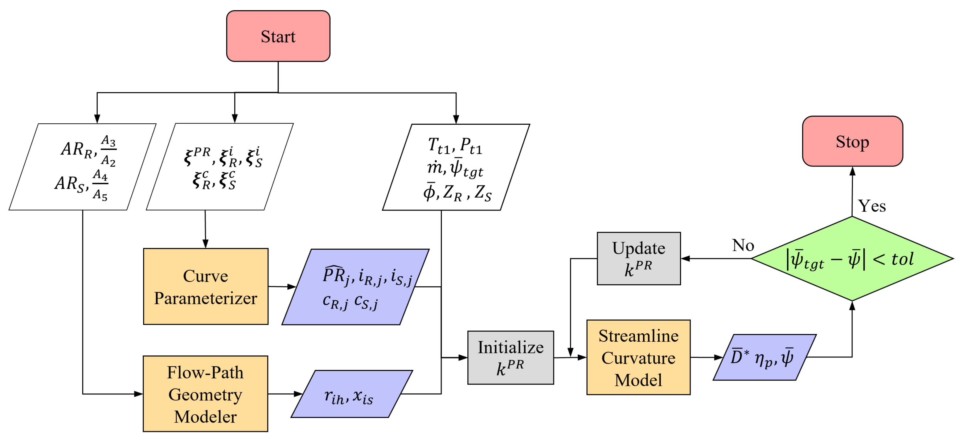
A flow chart of the overall model setup is shown
Figure 1. The model consists of a process for the generation of the flow path geometry that defines the corner points of the domain, a process for representing the radial distributions of inputs as parametric curves, and a process representing the streamline-curvature program. The outputs of the two former processes are fed into the SLC program as inputs.
The flow path geometry, as illustrated in
Figure 2a, is defined in part by the hub-to-tip ratio
and the casing radius at the inlet station
. The entire flow path is divided into five subsections, the inlet-, the rotor-, the intermediate-, the stator-, and the outlet-duct. For each subsection, three design variables can be varied: (1) inlet height-to-length ratio; (2) inlet-to-outlet area ratio; and (3) casing hade angle. For the purpose of this study, the problem was further simplified by keeping the casing radius constant at a value of 1.0 m, the area ratio for the inlet and the outlet sections constant, and a fixed value of 3.33 on the height-to-length ratio for the intermediate duct. The area ratio of the intermediate duct is further iterated on until the tangent of the hade angle at the hub is the average of the corresponding rotor and stator values. This was performed to facilitate a smooth transition from the rotor leading edge to the stator trailing edge. As output from the flow path geometry module, the computational grid points at the hub and the casing curve for the SLC program are returned in terms of axial and radial coordinates
,
and
,
.
The commercial throughflow code SC90C is used for the fan stage performance predictions. The software implementation of the SLC equilibrium equations are based on the formulation by Denton [
8] with loss and deviation correlations as well as annulus wall blockage prediction from Wright and Miller [
9]. Spanwise mixing is further modeled using the equations of Gallimore [
10].
The SLC program takes hub and the casing coordinates as input which specifies the location and orientation of the quasi-orthogonal planes. The operating condition for the stage is specified by setting the mass flow through the stage , the radial distributions of stagnation temperature at the inlet (), stagnation pressure at the inlet (), swirl angle at the inlet (), and the rotor rotational speed. Design variables for each blade row are specified accordingly for both the rotor and stator: spanwise distributions of aerodynamic chord length ( and ), maximum profile thickness ( and ), incidence angle ( and ), and leading edge radius ( and ) as well as the trailing edge radius (, and ). As part of the internal inverse design procedure of SC90C, the user has the option to specify the spanwise distribution of the stage pressure ratio () and stator outlet swirl angle , instead of explicitly specifying the stagger or the camber angle for the rotor and the stator blade row. For each blade row, the number of blades ( and ) and tip clearance ( and ) are also specified.
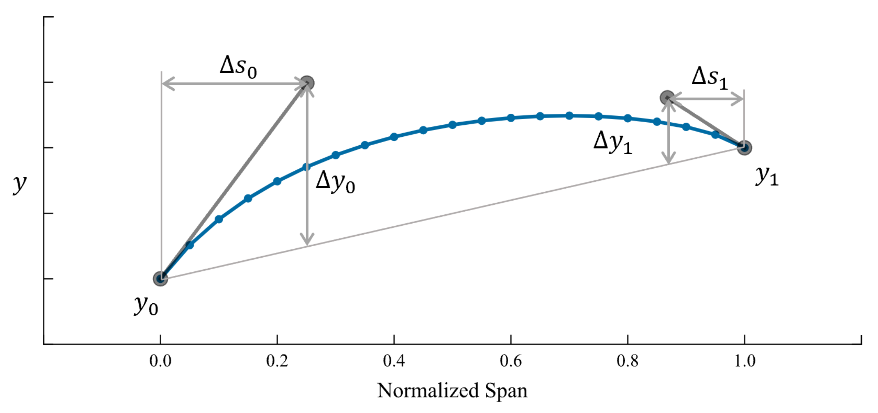
Variables distributed along the spanwise direction are parameterized with cubic Bézier curves [
11]. The parameterization defines the Bézier control-polygon with six degrees of freedom in total, as illustrated in
Figure 3. With
and
being equal to zero, the parameterization is reduced to a linear interpolation between the hub and the casing values.
2.2. Streamline Curvature Loss Correlations
Here, a brief review of the loss modeling implemented in SC90C is given as follows. For a more detailed description, the reader is referred to the paper by Wright and Miller [
9] that describes the loss and deviation correlations as well as the blockage prediction that the method used herein is largely based upon. Stations 1 and 2 used in this section refer to the inlet and the outlet of a single blade row, respectively. Stagnation properties, velocities, and flow angles are further expressed in a frame-of-reference relative to the blade passage, unless stated otherwise. The method estimates the blade row total pressure loss by dividing the overall pressure loss into a sum of three loss sources, representing the profile, endwall, and shock loss, respectively. Correlations are based on the pressure loss coefficient defined as the difference in the total pressure from the inlet to the outlet of the blade row divided by the dynamic pressure, i.e.,
In the following paragraphs, a short description is given for the correlations associated to each loss sources.
Profile loss is first determined for the minimum loss incidence condition according to Lieblein [
12],
where the wake momentum thickness per chord
is a function of Lieblein’s equivalent diffusion factor
and the inlet relative Mach number. The diffusion factor is further corrected for thickness-to-chord effects established for double circular arc (DCA) airfoils and is expressed accordingly:
The profile loss at a general incidence angle is obtained with correlations for an incidence angle at minimum loss, choke, and stall condition, together with generalized curves relating the offset in incidence from the minimum loss value to an associated increase in profile loss.
Endwall loss. Effects due to the endwall boundary layer and the interaction with the blade boundary layer are correlated against the aspect ratio, blade loading, and tip clearance, in accordance with Wright and Miller [
9]. The correlation is then extended to a 2D flow assuming a parabolic distribution along the span. The undistributed endwall loss coefficient is expressed accordingly:
where Lieblein’s diffusion factor
D is used to take into account the effect of blade loading, defined as:
Calibration of empirical coefficients in the formulation of Equation (
4) were performed by Wright and Miller [
9] against data on single and multistage compressors.
Shock loss. For inlet relative Mach numbers above 1.0, the pressure loss due to the formation of shock waves inside the blade passage is approximated by a theoretical loss model described by Schwenk et al. [
13]. The resulting pressure loss is taken as a fraction of the pressure loss calculated over a normal shock superseded by a representative passage Mach number. For inlet Mach numbers between 0.8 and 1.0, the shock loss is taken as a proportion of the loss calculated at
.
Reynolds number effects. Profile and endwall losses calculated according to the procedure above are taken to be valid for a Reynolds number of
. Effects of the Reynolds number is accounted for by applying corrections to the nominal values of profile and endwall loss coefficient. It is assumed that the flow is hydraulically smooth up to a Reynolds number of
and that losses are invariant with respect to the Reynolds number beyond that value. It is further assumed that the transition from the laminar to hydraulically smooth turbulent flow occurs at a Reynolds number of
. In detail, the corrections are calculated for the three regions accordingly
2.3. Blade Loading Parameter
Requirements on the stall margin has a strong influence on the fan design point efficiency. For the purpose of this study, a measure of aerodynamic loading evaluated in the design point will be used as a proxy for the stall margin. A normalized parameter based on the stall criteria for blade profiles by Aungier [
14] was used as a measure of aerodynamic loading over a given blade section. Stall occurs if the equivalent velocity ratio
falls below the critical value, i.e.,
with
defined as in Equation (
3). The equivalent velocity ratio is further defined from the row inlet and outlet static pressures and the total pressures in the blade section relative frame
The normalized aerodynamic loading at a given spanwise position is then simply defined as
where
is the right-hand side of the inequality in Equation (
7). It is further assumed that stall for a blade-row occurs when the loading parameter is greater than or equal to one for at least
of the total inlet annulus area. A representative value for the aerodynamic loading of the entire blade denoted by
is then chosen as the 75% percentile value. Calculation steps are as follows:
Calculate the loading parameter for each streamline and the associated annulus area fraction.
Sort the streamlines by loading parameter.
Calculate the cumulative distribution of the area with respect to the loading parameter.
Calculate the loading parameter at a cumulative area fraction of .
The stage-wise aerodynamic loading is taken as the maximum of the rotor and the stator values, i.e.,
2.4. Optimization Setup
The optimization problem considered here can be described as a multi-parametric multi-objective optimization problem. In shorthand, it reads
with
objectives and
optimization parameters given in detail in Equations (
10) and (11), and the
design variables listed in
Table 2.
For the purpose of this study, the parametric optimization is performed by simply running multiple constrained optimizations independently by varying values on the selected parameters in Equation (11). Parameter values for each optimization were generated by means of random Latin-hypercube-sampling (LHS). The number of sampling points—and thereby the number of independent optimizations that were required to be performed—was chosen as the number of data points required to exactly define a multivariate second-order polynomial in
n variables, which is given by the following expression:
With the 4 scalar optimization parameters defined in Equation (11), Equation (
12) yields 15 required sampling points. It should be noted that following this rule of thumb for deciding the number of sampling points by no means guarantees a sufficient sampling size in general, but was deemed to be enough for the purpose of demonstrating the optimization approach. Value ranges for each parameter and design variable as well as values for additional fixed value parameters are shown in
Table 2. For the optimization, a standard NSGAII algorithm was used. Each optimization was set to run for 200 generations with 100 offsprings per generation and a total population size of 500.
2.5. Surrogate Modeling
The goal with the surrogate models is to predict stage polytropic efficiency and the required rotor solidity for Pareto optimal designs as an analytical function of the optimization parameters and the blade loading parameter. The surrogate models then take the following form:
The results obtained from the preceding parametric optimization with values of efficiency and rotor solidity at corresponding values for the optimization parameters as well as blade loading are then used as training data for the surrogate model. A standard Kriging method is chosen for this purpose.
2.6. Engine Systems Modeling
The resulting surrogate models of the first part are, in the second part of this study, integrated into an engine cycle performance model and coupled with a simplified weight model. The main objectives of this investigation is to illustrate a use case for—and the possible implications of—including a higher degree of fan-stage parameter interdependency into the conceptual design of a turbofan engine. A design space exploration is carried out for one operating condition with fixed values on net thrust and fan diameter. Fan-stage design variables that could have been included into the analysis but were held constant are the rotor aspect ratio and the fan stage blade loading parameter. With regard to the additional engine cycle parameters, the overall pressure ratio and the turbine inlet temperature were also held constant. Three design variables were then considered for this investigation, namely the fan-face Mach number, the relative tip Mach number, and the jet velocity ratio. The fan-face Mach number will influence the fan-stage efficiency and the required solidity, but it will in this case also specify the total mass flow through the engine and by extension the specific thrust. The relative tip Mach number will for a given axial Mach number, fan rotor hub-tip-ratio, and diameter, specify the blade speed and by extension the stage loading and flow coefficient, and will therefore have an effect on both the fan stage weight and efficiency. The jet velocity ratio is here defined as the ratio of the specific gross thrust between the bypass stream and the core stream. It is related to the relative amount of power that is transferred to the bypass stream from the core and has, for a fixed thrust requirement and fan diameter, a comparatively large influence on the size and weight of the core and the thrust-specific fuel consumption.
Appropriate values for the constant parameters and baseline values for the design variables are determined from a baseline engine configuration. For this purpose, a geared turbofan representative of a Pratt & Whitney PW1133G in terms of thrust requirement and component technology level was chosen. Since the SLC model used in part one of this study was calibrated against data on designs that by today’s standards would be considered outdated technology, the predicted magnitudes of efficiency and rotor solidity very likely differ from state-of-the-art technology. To be more consistent with the technology level of a state-of-the-art engine, the baseline cycle parameters for the performance model—including an initial estimate of the fan-stage efficiency—were calibrated against open data using a method similar to the one described in [
15].
Table 3 shows the operating conditions of the selected design point, the thrust requirement, as well as baseline parameters for the fan-stage. The efficiency and solidity calculated by the surrogate models are normalized to meet the estimated baseline values at the corresponding values of the flow coefficient, stage loading, fan-face Mach number, rotor aspect ratio, and blade loading parameter.
Below, brief descriptions of the modeling setup for the engine dry weight and cycle performance are given as follows.
2.6.1. Engine Performance
The thermodynamic calculations of the inlet, the outer (bypass) part of the fan, and the bypass nozzle are evaluated with PyCycle [
16], which is an open source thermodynamic cycle modeling library intended for jet engines written in Python and built on top of the openMDAO framework [
17]. For improved flexibility and computational speed, the performance of the engine core is represented by a spline-surface. The spline-surface model calculates the core gross thrust and required fuel flow. It takes as input the power extracted from the low-pressure turbine to the outer part of the fan, core mass-flow, and pressure ratio of the inner part of the fan. The core performance data are sampled from the Chalmers in-house cycle performance code GESTPAN [
18]. Additional compatibility between the core model and the rest of the engine as well as the efficiency surrogate model is solved for with the Newton method supplied by the openMDAO framework.
2.6.2. Engine Dry Weight
The dry engine weight is broken down into the weight of the fan-stage, the speed-reduction gearbox, and the core. Fan stage weight is further divided into a blade-set weight and three additional constituents representing the weight of the containment ring, the structure, and the disc, related to the fan diameter
, number of rotor blades
, rotor solidity
, and the maximum rotor blade tip speed
. The proportionality relationships are assumed to be as follows
The gearbox weight is assumed to be directly proportional the maximum permissible output torque. The estimated baseline values for the blade tip speed and gearbox output torque are used to calculate a ratio to each maximum value. These ratios are then held constant as the corresponding values in the design point are varied. It is important to note that the dimensioning point may not be the chosen design point for this study and that a proper multi-point analysis is necessary to better estimate the relationship between maximum permissible values and design point values.
The core baseline weight is calculated from open data on an engine dry weight for the PW1133G engine together with the resulting estimates of the baseline fan-stage and gearbox weights. The core weight is then assumed to be directly proportional to the core mass flow as the design value is being varied. Note that when the required power output from the low-pressure turbine is increased for the same core mass flow, the turbine weight typically increases, either due to heavier discs as a result from a higher rotational speed or an additional turbine stage. This effect has not been included here.
3. Results
The results section is divided into two sub-sections, each covering the outcome of the two parts of the study, respectively, i.e., the fan-stage parameter interdependency study and the design space exploration of the engine systems model.
3.1. Part: 1—Fan-Stage Parameter Interdependencies
The time taken for the SLC model alone to converge to a single design point on a standard desktop PC is in the order of 2.0 s. The time required to run 200 generations with 100 offspring per generation and an initial sampling of 500 individuals, i.e., one optimization, therefore amounts to about six core hours. The time taken to train the final surrogate models on a dataset of about 600 individuals was in the order of minutes.
A prediction profiler demonstrating the relation of the stage polytropic efficiency with respect to the optimization parameters and the blade loading parameter is shown in
Figure 4. This illustrates the variation of efficiency, predicted by the surrogate model, when each parameter is varied around a given reference point, while the remaining parameters are kept fixed at their respective reference values. The reference values in
Figure 4, marked by the intersection between the two dashed lines in each subplot, are chosen accordingly:
,
,
, and
.
When the fan-face Mach number
is increased above 0.6, the stage efficiency falls rapidly, while the variation is small for lower values. Since a high mass flow per unit of frontal area is advantageous from the standpoint of both fan weight and nacelle drag, it is likely that some penalty in stage efficiency could be accepted if the fan-face Mach number is increased beyond the value for peak efficiency. Values of up to and around Mach 0.65 are typical for high bypass turbofans of the previous generation [
1,
2]. With fan weight being roughly proportional to the fan-face area, going from 0.55 to 0.65 in Mach number has the potential to yield more than a
reduction in both the fan component weight and nacelle wetted area.
A decrease in the rotor axial aspect ratio results in an increased stage efficiency. This could possibly be attributed to a reduction in the thickness-to-chord ratio that may influence the efficiency in the following ways: (1) a decrease in profile losses due to a reduction in the trailing edge momentum thickness; and (2) a reduced strength of the passage shock in the tip region due to reduced blockage. The weak dependency on thickness-to-chord on the blade loading parameter may also contribute slightly.
When the flow coefficient is reduced from the reference value of 0.8, a reduction in the predicted stage efficiency can be observed. With the axial Mach number at the fan-face held fixed, a reduction in the flow coefficient is equivalent to an increase in the relative Mach number. With a fan-face relative Mach number expressed as and a flow coefficient at the tip expressed as , a relative Mach number at the tip can be estimated to around 1.082 for the reference design. The associated drop in stage efficiency going from a flow coefficient of 0.8–0.625 with axial Mach number held constant at 0.55 matches very well the predicted drop in efficiency when going from an axial Mach number of 0.55 to 0.675 keeping the flow coefficient constant at 0.8. For each of these two cases, the corresponding relative Mach numbers at the tip increases from the reference value of 1.082 to 1.313 and 1.327, respectively, which may indicate that a large part of the loss increase associated with the decrease in flow coefficient can be attributed to an increase in the strength of the passage shock-wave.
Regarding the blade loading parameter, a maximum can be seen close to the reference point value of 0.88. The efficiency is seen to have a maximum close to the reference blade loading parameter of 0.88. The decrease in efficiency as the blade loading parameter is further increased may be an effect of extrapolation since the data from any potential individuals in this part of the design space are likely Pareto-dominated and therefore filtered away by the sorting algorithm already during optimization. In the case of such a maximum occurring at low values of blade loading, this approach may exclude feasible designs that could otherwise be of interest. Since solidity has a strong influence on weight, a design with lower solidity at the expense of efficiency might be preferred due to the reduction in weight provided that the stall/surge margin is sufficiently high. One way of sampling this part of the design space during a parametric optimization could be to implement a modified selection procedure to enforce a spread in the blade loading parameter without specifying it as a conventional objective with a predetermined preference ordering.
The stage loading versus efficiency trend can be seen in the left-most subplot in
Figure 4. Unlike the common trend seen in the literature on conceptual design, the efficiency seems to be increasing with stage loading for the most part. A possible explanation for the trend observed here may be that, as the rotor-relative tip Mach number increases, the optimal stage loading will increase. For given stagnation properties at the inlet, the given flow coefficient and zero inlet swirl, the lost work as a fraction of the useful work input is proportional to the entropy loss coefficient divided by the stage loading
where
Assuming that the entropy loss coefficient can be split into two components, where
represents shock losses that are independent of stage loading, and
represents the profile, endwall, and mixing losses (“subsonic” losses) that are independent of the Mach number. Taking the derivative of Equation (
18) and setting it as equal to zero will then yield the following expression for the point of optimal stage loading
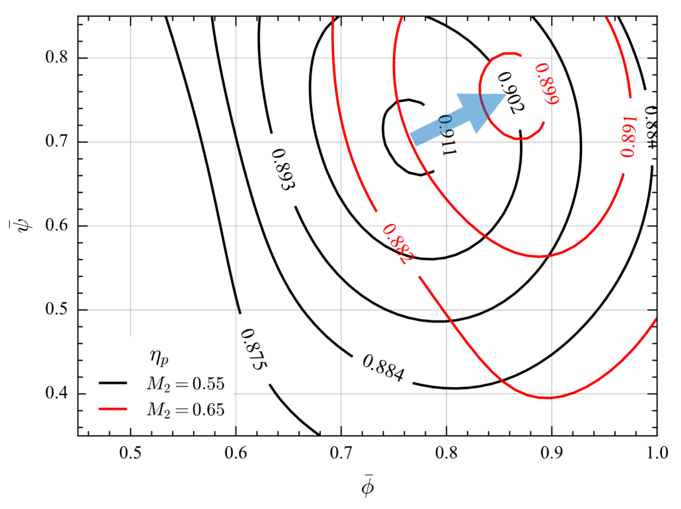
If
increases (by, for instance, increasing the inlet Mach number holding the flow coefficient constant), through Equation (
20), the optimal stage loading should also increase, as can be seen in
Figure 5. For designs with high mass flow rate per unit frontal area and low-stage loading, reducing the strength of the passage shock wave by sweeping the blade may be of importance. Blade sweep is here more important than for highly loaded fans where no noticeable effect in efficiency from lean and sweep was found according to Denton and Xu [
19]. Blade sweep was not considered as a design parameter in the present study.
3.2. Part: 2—Engine Performance and Weight
The design space of the engine systems model was explored by performing both parameter sweeps and a trade-off study. The parameter sweeps were carried out in order to demonstrate the individual effect on the objectives from variations in each design variable and to justify the observed trends based on previous modeling assumptions. Optimizations were carried out in order to investigate the implications on the trade-off between the two objectives, engine dry weight, and specific fuel consumption for Pareto-optimal designs when more fan-stage parameter interdependencies are included. The two following subsections present the results and their interpretations for the parameter sweep and the trade study, respectively.
3.2.1. Engine Model Parameter Sweep
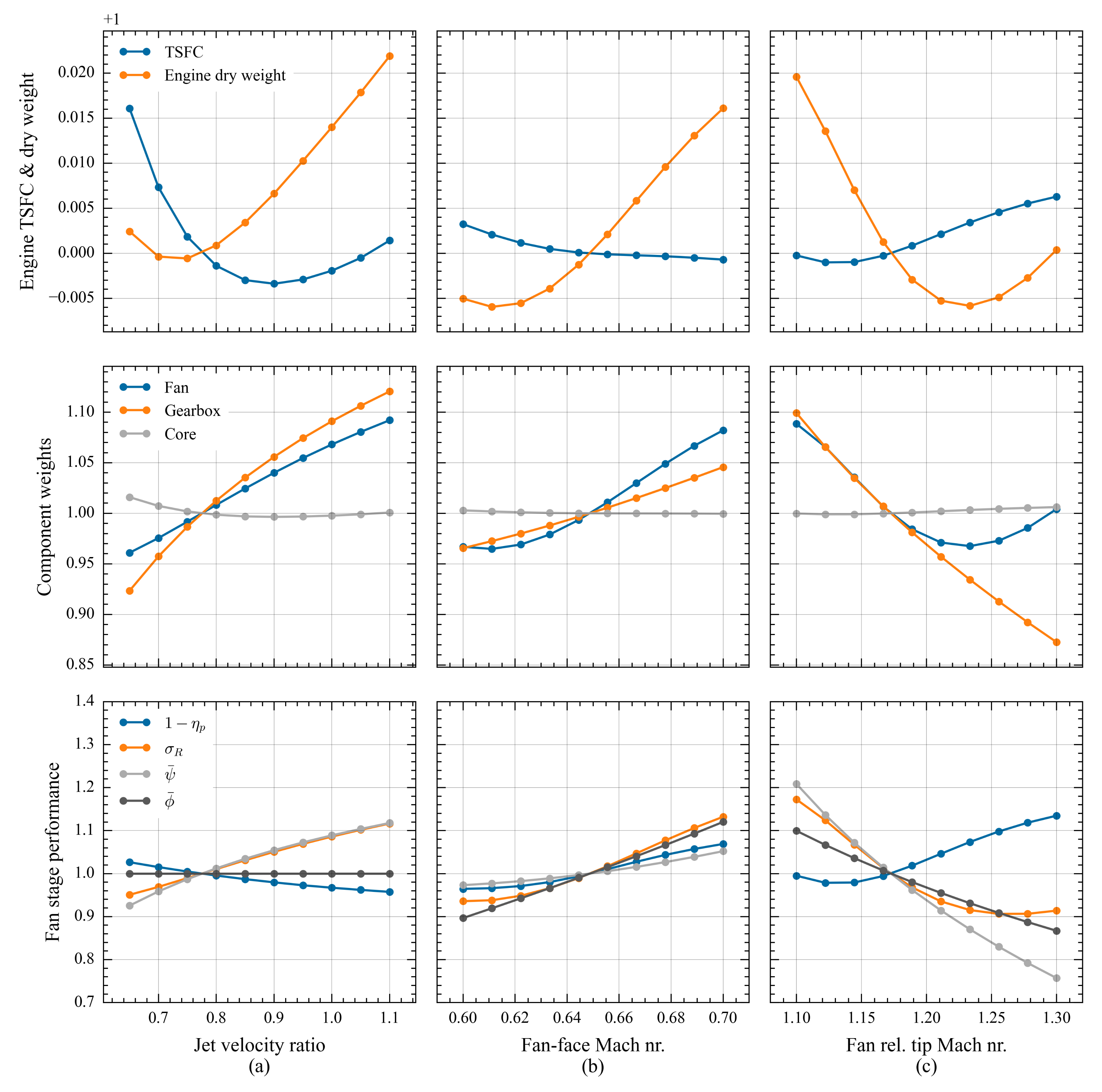
For the parameter sweep, the three design variables, namely the jet velocity ratio, fan-face Mach number, and rotor relative tip Mach number, were varied independently around their baseline values. The response in terms of engine dry weight and thrust specific fuel consumption as well as component weights and fan-stage performance are shown in
Figure 6. The three columns (a), (b), and (c) of
Figure 6 show the results from each individual parameter sweep, respectively. Similarly to the prediction profiler in
Figure 4, when one of the design variables is varied, the others are held fixed at their respective baseline value.
A few things can be concluded about the parameter sweeps. With regard to the variation in jet velocity ratio, a TSFC optima can be seen around 0.9. The slight increase in fan stage efficiency as the jet velocity ratio increases most likely moved the TSFC optima towards a slightly higher value. The increase in fan efficiency can be traced to an increase in stage loading as more power is transferred to the fan together with the efficiency vs. stage-loading trend predicted by the surrogate model. The existence of an engine dry weight optima can be explained by a balance between a predicted increase in fan-stage weight and a decreasing core weight. The increasing fan weight is likely due to the stage loading increase and the accompanying increase in solidity required to maintain the same average blade loading. More power required by the fan with a constant rotational speed will result in an increased torque which can explain the observed increase in gearbox weight.
As the fan-face Mach number increases, there is an overall decrease in TSFC within the selected design variable bounds, although with diminishing returns due to an accompanying decrease in fan-stage efficiency predicted by the surrogate model. An engine weight optima can be observed around 0.61 and seem by all accounts to be a result of the fan weight optima found at the same fan-face Mach number. The fan weight optima can be explained by a balance between the effects of a decreasing blade speed and the increase in required solidity predicted by the surrogate model.
As a relative tip Mach number increases, the TSFC increases since the propulsive efficiency is approximately constant, and a steady decrease in fan efficiency is likely due to increased shock losses. No optima were found within the given parameter range. As the relative Mach number decreases beyond the baseline value, the fan efficiency and thereby TSFC can be observed to reach an optima. An engine weight and fan weight optimum is seen around 1.23 which could be explained by a balance between a steadily increased blade speed requiring a heavier disc and containment ring and a reduced required rotor solidity predicted by the surrogate model.
3.2.2. Engine Model Trade-Off Study
Two multi-objective optimizations were carried out. One with only a jet velocity ratio included as a design variable with the other two was held fixed at their baseline values and another optimization including all three design variables. The optimizations were performed with an upper constraint on one of the objectives—in this case, the engine dry weight—while performing a number of single objective optimizations minimizing TSFC. To sample a Pareto-front, each single objective optimization was performed with progressively higher values on the engine dry weight constraint. The two resulting Pareto-frontiers can be seen in
Figure 7a with the corresponding design variable values shown in
Figure 7b. For the optimization with only jet velocity ratio as a design variable, there is a maximum variation of 0.68% in TSFC within the trade-space and a corresponding variation of 0.71% in the engine dry weight. When the fan-face Mach number and relative tip Mach number are included, the variations increase to 0.85% and 2.0%, respectively. As can be noted, the trade-space variation increases for both objectives but more so for the engine weight than the TSFC in this case. Not including the influence of the fan-face Mach number and relative tip Mach number on the fan efficiency and required rotor solidity, will therefore likely result in an under-predicted engine weight penalty for a given improvement in TSFC. The observed response in terms of the design variables when moving along the Pareto-front in the direction of the reduced TSFC is that the jet velocity and fan-face Mach number is increasing and the relative tip Mach number is decreasing. The design variable ranges within the trade-space for this particular example are 15.59%, 2.2%, and 6.0%, for jet velocity ratio, fan-face Mach numner and relative tip Mach number respectively.
4. Discussion
This study demonstrates the use of parametric optimization applied to the streamline curvature method to explore parameter interdependencies related to fan-stage aero-thermodynamic performance. The design space exploration on the component level is supported by surrogate models trained on the data produced by the parametric optimizations. The study ends with a use case, successfully demonstrating how the surrogate models can be integrated into an engine systems model to explore the trade-off between engine weight and specific thrust.
The parametric optimization campaign was initialized by generating the parameter values by means of Latin-hypercube sampling. The chosen parameters for this purpose were stage loading, flow coefficient, rotor aspect ratio, and fan-face Mach number. For each sampling point, a two-objective optimization was carried out on a streamline curvature model with stage polytropic efficiency and a blade loading parameter as the objectives. The resulting set of the Pareto optimal designs were then used as training data to generate a surrogate model for polytropic efficiency in terms of the four parameters and the blade loading as independent variables. Upon the realization that the rotor solidity correlated relatively well with the blade loading in all sampling points, a surrogate model for rotor solidity in terms of the same five parameters was also generated.
It should be pointed out that, when entirely relying on throughflow predictions for the compressor performance, heavily based on correlations, the accuracy of the results will be highly dependent on the calibration of empirical coefficients. As reported in Wright and Miller [
9], some degree of calibration of the endwall and the shock loss model was performed. These calibrations were, however, only performed on a meanline basis. Additional calibrations and decisions about implementation-specific details have therefore been made by the developers of the software that the authors have little to no knowledge about. Another aspect of the validity of the results that is important to stress is that the modeling simplifications of a conventional correlation-based throughflow method will set a limit on how well actual trends can be captured. The shock loss model employed here is a gross simplification of the actual flow within a blade passage and could at best be expected to capture overall trends in the efficiency Mach number relationship. Since the loss model also treats the loss associated with boundary-layers and shock-waves as linearly independent, the effects of the shock-wave boundary–layer interactions that are known to have a large influence on performance will not be captured very well. The precise rate of change of the efficiency Mach number relationship will therefore be very difficult to capture with this method. The approach to generate a lower-order surrogate model of an SLC model through parametric optimization—as demonstrated here—could, however, also be applied to a model of higher fidelity.
The overall trends predicted by the surrogate models were to some extent justified with physical reasoning and by comparison with common guidelines from the literature. Observed trends between efficiency, fan-face Mach number, and stage loading implied that shock losses may negatively impact efficiency to a larger extent when stage loading is reduced. This could imply that means to reduce the strength of the passage shock wave such as blade sweep might be of importance for designs with low-stage loading. With regard to the choice of the blade loading as an objective during the parametric optimizations, this could have the effect that designs which may be optimal in a global sense are excluded. This study therefore highlights the need for optimization algorithms that can more efficiently treat parameters with unknown preference ordering.
Several geometric features not included in the interdependency study for this paper could be of interest to include in future work, such as the rotor inlet hub-tip-ratio, rotor, and OGV maximum profile thickness and tip clearance. Including the diameter as an independent parameter in order to account for Reynolds number effects and choosing a more representative baseline domain in terms of the hub and the casing contours are additional aspects worth considering. Parameter interdependencies representative for state-of-the-art and future fan technology would require the high-fidelity method used during the parametric optimization to be sensitive to more geometric features. If the effects from detailed variations in the blade profile shapes should be taken into account, a blade-to-blade solver coupled with a throughflow solver could be justifiable. If 3D features such as lean and sweep are considered important, then the 3D RANS of the entire blade passage would most likely be required. For the parametric optimization to be computationally feasible in this case, without having to sacrifice too much in terms of the parameter sample size, a surrogate assisted approach would probably also be necessary for this purpose.
The second part of this study demonstrates the importance of having a multidisciplinary perspective when setting up the design of an experiment to evaluate the fan-stage aero-thermodynamic performance with a higher fidelity method. In the case of a fan-stage in a high-bypass low-specific thrust turbofan, being able to predict the rotor solidity required to maintain a given average blade loading was proven to be just as important as predicting the fan stage efficiency when it comes to evaluating the trade-off between the engine weight and thrust-specific fuel consumption. Additional considerations for future work include extending the low-order model to incorporate relevant effects on the off-design performance characteristic as well. This could potentially facilitate a direct coupling of the engine model with aircraft design and mission analysis to investigate how fan parameters affect operational flexibility.
Author Contributions
Conceptualization, O.S.; methodology, O.S. and A.L.; software, O.S., T.G. and C.X.; validation, O.S., A.L. and C.X.; formal analysis, O.S.; investigation, O.S.; resources, C.X., A.L. and T.G.; data curation, O.S. and A.L.; writing—original draft preparation, O.S.; writing—review and editing, O.S., C.X. and A.L.; visualization, O.S.; supervision, C.X. and A.L.; project administration, C.X., A.L. and T.G.; funding acquisition, A.L. and T.G. All authors have read and agreed to the published version of the manuscript.
Funding
This research work was funded by the Swedish National Aviation Engineering Research Program, NFFP, grant number: 2023-01193.
Institutional Review Board Statement
Not applicable.
Informed Consent Statement
Not applicable.
Data Availability Statement
Data are contained within the article.
Acknowledgments
This research work was supported by Swedish Armed Forces, the Swedish Defense Material Administration and the Swedish Governmental Agency for Innovation Systems, VINNOVA.
Conflicts of Interest
Anders Lundbladh was employed by the company GKN Aerospace Sweden. The remaining authors declare that the research was conducted in the absence of any commercial or financial relationships that could be construed as a potential conflict of interest.
Nomenclature
| Abbreviations |
| AR | Aspect ratio |
| DCA | Double circular arc |
| HTR | Hub-tip-ratio |
| PR | Pressure ratio |
| LHS | Latin hyper-cube sampling |
| SLC | Streamline curvature |
| TSFC | Thrust specific fuel consumption |
| Symbols |
| A | Area, (m) |
| c | Chord, (m) |
| Fan diameter, (m) |
| D | Lieblein’s diffusion factor, (-) |
| Normalized blade loading, (-) |
| Equivalent diffusion, (-) |
| h | Specific enthalpy, () |
| i | Incidence angle, () |
| Mass flow, () |
| P | Pressure, (Pa) |
| Radial and axial coordinate, (m) |
| Leading and trailing edge radius, (m) |
| s | Specific entropy, () |
| T | Temperature, (K) |
| t | Max profile thickness, (m) |
| V | Velocity, (m/s) |
| Whirl velocity, (m/s) |
| U | Rotor blade velocity, (m/s) |
| Equivalent velocity ratio, (-) |
| W | Weight (mass), (kg) |
| Z | Blade count |
| Flow angle, () |
| Tip clearance, (m) |
| Polytropic efficiency, (-) |
| Solidity, (-) |
| Stage loading, (-) |
| Flow coefficient, (-) |
| Design variable vector |
| Optimization parameter vector |
| Entropy loss coefficient, (-) |
| Wake momentum thickness (m) |
| Camber angle (rad) |
| Stagger angle (rad) |
| Pressure loss coefficient |
| Subscripts |
| 1, 2, 3 … | Station number |
| Parameter at the hub |
| Meridional and normal grid index |
| R | Rotor |
| S | Stator |
| Parameter at the blade tip (or casing) |
| t | Total/stagnation property |
| Parameter target value |
| Radial and axial component |
References
- Walsh, P.P.; Fletcher, P. Gas Turbine Performance, 2nd ed.; Blackwell Science Ltd.: Oxford, UK, 2004. [Google Scholar]
- Grieb, H. Projektierung von Turboflugtriebwerken; Birkhäuser: Basel, Switzerland, 2003. [Google Scholar]
- Kurtzke, J.; Riegler, C. A new compressor map scaling procedure for preliminary conceptional design of gas turbines. In Proceedings of the ASME Turbo Expo 2000: Power for Land, Sea, and Air, Munich, Germany, 8–11 May 2000; Volume 1. [Google Scholar]
- Converse, G.L.; Giffin, R.G. Extended Parametric Representation of Compressor Fans and Turbines. Volume 1: CMGEN User’s Manual; National Aeronautics and Space Administration Lewis Research Center: Cleveland, OH, USA, 1984. [Google Scholar]
- Turner, M.G.; Reed, J.A.; Ryder, R.; Veres, J.P. Multi-Fidelity Simulation of a Turbofan Engine With Results Zoomed Into Mini-Maps for a Zero-D Cycle Simulation. In Proceedings of the ASME Turbo Expo 2004: Power for Land, Sea, and Air, Vienna, Austria, 14–17 June 2004; Volume 2. [Google Scholar]
- Templalexis, I.; Alexiou, A.; Pachidis, V.; Roumeliotis, I.; Aretakis, N. Direct coupling of a two-dimensional fan model in a turbofan engine performance simulation. In Proceedings of the ASME Turbo Expo 2016: Turbomachinery Technical Conference and Exposition, Seoul, Republic of Korea, 13–17 June 2016; Volume 3. [Google Scholar]
- Sjögren, O.; Grönstedt, T.; Lundbladh, A.; Xisto, C. Fan Stage Design and Performance Optimization for Low Specific Thrust Turbofans. In Proceedings of the 15th European Turbomachinery Conference, Paper n. ETC2023-272, Budapest, Hungary, 24–28 April 2023; Available online: https://www.euroturbo.eu/publications/conference-proceedings-repository/ (accessed on 20 July 2023).
- Denton, J.D. Throughlow Calculations for Transonic Axial Flow Turbines. J. Eng. Gas Turbines Power 1978, 100, 212–218. [Google Scholar] [CrossRef]
- Wright, P.I.; Miller, D.C. An improved compressor performance prediction model. In Proceedings of the IMechE Conference Turbomachinery: Latest Developments in a Changing Scene, London, UK, 19–20 March 1991. [Google Scholar]
- Gallimore, S.J. Spanwise Mixing in Multistage Axial Flow Compressors: Part II—Throughflow Calculations Including Mixing. ASME J. Turbomach. 1986, 108, 10–16. [Google Scholar] [CrossRef]
- Mortenson, M.E. Mathematics for Computer Graphics Applications, 2nd ed.; Industrial Press Inc.: New York, NY, USA, 1999. [Google Scholar]
- Lieblein, S. Loss and stall analysis of compressor cascades. J. Basic Eng. 1959, 81, 387–397. [Google Scholar] [CrossRef]
- Schwenk, F.C.; Lewis, G.W.; Hertman, M.J. A Preliminary Analysis of the Magnitude of Shock Losses in Transonic Compressor (No. NACA-RM-E57A30); Lewis Flight Propulsion Laboratory: Cleveland, OH, USA, 1957. [Google Scholar]
- Aungier, R.H. Axial-Flow Compressors: A Strategy for Aerodynamic Design and Analysis; The American Society of Mechanical Engineers: New York, NY, USA, 2003. [Google Scholar]
- Sjögren, O.; Xisto, C.; Grönstedt, T. Estimation of Design Parameters and Performance for a State-of-the-Art Turbofan. In Proceedings of the ASME Turbo Expo 2021: Turbomachinery Technical Conference and Exposition, Virtual, Online, 7–11 June 2021; Volume 1. [Google Scholar]
- Hendricks, E.S.; Gray, J.S. pyCycle: A Tool for Efficient Optimization of Gas Turbine Engine Cycles. Aerospace 2019, 6, 87. [Google Scholar] [CrossRef]
- Gray, J.S.; Hwang, J.T.; Martins, J.R.R.A.; Moore, K.T.; Naylor, B.A. OpenMDAO: An open-source framework for multidisciplinary design, analysis, and optimization. Struct. Multidiscip. Optim. 2019, 59, 1075–1104. [Google Scholar] [CrossRef]
- Grönstedt, T. Development of Methods for Analysis and Optimization of Complex Jet Engine Systems. Ph.D. Thesis, Chalmers University of Technology, Gothenburg, Sweden, 2000. [Google Scholar]
- Denton, J.D.; Xu, L. The Effects of Lean and Sweep on Transonic Fan Performance. In Proceedings of the ASME Turbo Expo 2002: Power for Land, Sea, and Air, Amsterdam, The Netherlands, 3–6 June 2002; Volume 5, pp. 23–32. [Google Scholar]
| Disclaimer/Publisher’s Note: The statements, opinions and data contained in all publications are solely those of the individual author(s) and contributor(s) and not of MDPI and/or the editor(s). MDPI and/or the editor(s) disclaim responsibility for any injury to people or property resulting from any ideas, methods, instructions or products referred to in the content. |
© 2023 by the authors. Licensee MDPI, Basel, Switzerland. This article is an open access article distributed under the terms and conditions of the Creative Commons Attribution (CC BY-NC-ND) license (https://creativecommons.org/licenses/by-nc-nd/4.0/).


