1. Introduction
Axial turbines are the most common turbine configuration for electric power generation and propulsion systems, including: open Brayton cycles [
1], closed Brayton cycles using helium [
2] or carbon dioxide at supercritical conditions [
3], and Rankine cycles using steam [
4] or organic working fluids [
5]. In addition, they are also used in cryogenic applications such as gas separation processes and liquefaction of natural gas [
6]. Arguably, axial turbines owe their popularity to their versatility in terms of power capacity and range of operating conditions. The power capacity of axial turbines can vary from tens of kilowatts for small-scale Rankine power systems using organic fluids to hundreds of megawatts for large-scale steam and gas turbine power plants. In addition, the operating temperatures range from below −200 °C in some cryogenic applications to temperatures in excess of 1500 °C for some advanced gas turbines, whereas the operating pressures can vary from a few millibars at the exhaust of some steam turbines to hundreds of bars at the inlet of supercritical steam and carbon dioxide power systems.
The fluid-dynamic or aerodynamic design of axial turbines can be divided in several steps involving mathematical models of different levels of complexity ranging from low-fidelity models for the preliminary design (mean-line and through-flow models) to high-fidelity models for the detailed blade shape definition (solution of the Navier–Stokes equations with turbulence models) [
7]. Even if mean-line models are the simplest approach to analyze the thermodynamics and fluid dynamics of turbomachinery, they are still an essential step of the fluid-dynamic design chain because they provide the information required to use more advanced flow models [
8]. Mean-line models assume that the flow is uniform at a mean radius and evaluate the conditions at the inlet and outlet of each cascade using the balance equations for mass and rothalpy, a set of equations of state to compute thermodynamic and transport properties, and empirical loss models to evaluate the entropy generation within the turbine [
9]. In addition, to automate the preliminary design, it is possible to formulate the mean-line model as an optimization problem. This is especially advantageous to design new turbine concepts because it allows exploration of the design space in a systematic way and account for technical limitations in the form of constraints [
7].
Despite mean-line models being covered to some extent in turbomachinery textbooks [
1,
9], only some scientific publications present a comprehensive formulation of the preliminary design problem.
Table 1 contains a non-exhaustive survey of mean-line axial turbine models in the open literature. Some of the differences in the model formulation include: considering single-stage or multistage turbines, using restrictive assumptions such as repeating stages or not, using simplified equations of state or real gas fluid properties, and whether or not to account for the influence of the diffuser on turbine performance. In addition, some works formulate the preliminary design as an optimization problem and then solve it using gradient-based or direct search optimization algorithms, while other works formulate the design problem as system of equations and then do parametric studies to explore the design space. One of the recurring limitations of the scientific literature is that most mean-line models have not been validated against experimental data or CFD simulations. Finally, to the knowledge of the authors, no publication has made the mean-line model source code openly available to the research community and industry, with the notable exception of the
Meangen code by Denton [
8].
In this work, a mean-line model and optimization methodology for the preliminary design of axial turbines with any number of stages is proposed. The model is presented in
Section 2 and it was formulated to use arbitrary equations of state and empirical loss models and to account for the influence of the diffuser on turbine performance using a one-dimensional flow model from a previous publication [
10]. In addition,
Section 3 contains the validation of the model against experimental data from two well-documented test cases reported in the literature. After that, the design problem is formulated as a constrained optimization problem in
Section 4 and the proposed optimization methodology was applied to a case study from the literature in
Section 5 to assess the optimal design in terms of total-to-static efficiency, angular speed, and mean diameter. Finally,
Section 6 contains a sensitivity analysis of the case study with respect to: (1) isentropic power output, (2) tip clearance height, (3) minimum hub-to-tip ratio, (4) diffuser area ratio, (5) diffuser skin friction coefficient, (6) total-to-static pressure ratio, (7) number of stages and (8) angular speed and mean diameter to gain insight about the impact of these variables on the performance of the turbine and to extract general design guidelines. The authors would like to mention that the source code with the implementation of the mean-line model and optimization methodology described in this paper is available in an online repository [
11], see
Supplementary Materials.
2. Axial Turbine Model
Axial turbines are rotary machines that convert the energy from a fluid flow into work. An axial turbine is composed of one or more stages in series and each stage consists of one cascade of stator blades that accelerate the flow and one cascade of rotor blades that deflect the flow, converting the enthalpy of the fluid into work as a result of the net change of angular momentum. The kinetic energy of the flow at the outlet of the last stage can be significant and, for this reason, it is possible to install a diffuser to recover the kinetic energy and increase the turbine power output.
This section describes the axial turbine model proposed in this work. First, the geometry of axial turbines and the variables involved in the model are introduced. After that, the conventions used for the velocity triangles are explained. Finally, the design specifications (boundary conditions) and the mathematical model for the axial turbine is described. This mathematical model is composed of three sub-models that are used as building blocks: (1) the cascade model, (2) the loss model, and (3) the diffuser model. In
Section 4 these sub-models are used to formulate the turbine preliminary design as a nonlinear, constrained optimization problem.
2.1. Axial Turbine Geometry
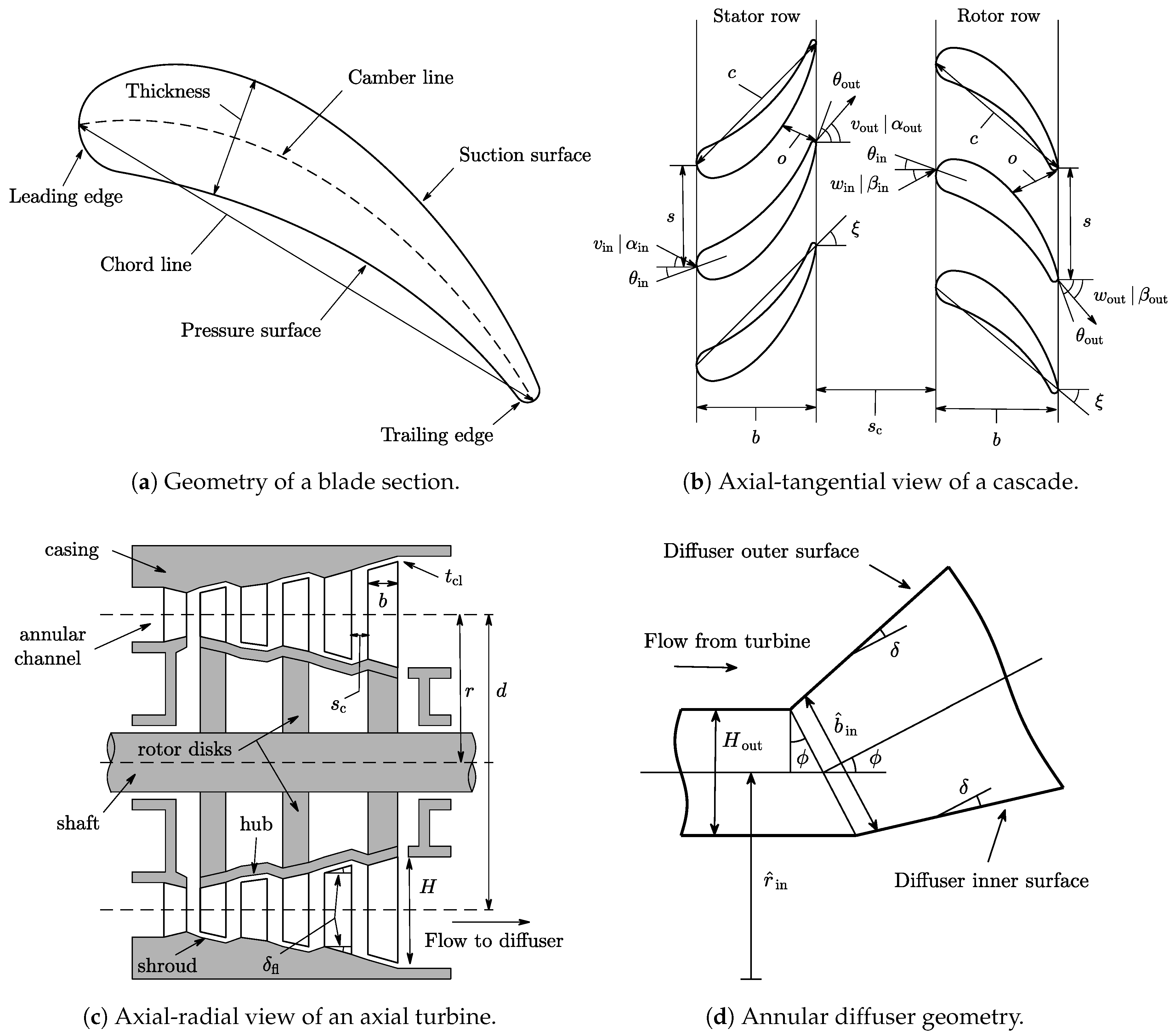
The geometry of a turbine blade is shown in
Figure 1a. Blades are characterized by a mean camber line halfway between the suction and the pressure surfaces. The most forward point of the camber line is the leading edge and the most rearward point is the trailing edge. The blade chord
c is the length of the straight line connecting the leading and the trailing edges. The blade thickness is the distance between the pressure and suction surfaces, measured perpendicular to the camber line. The aerodynamic performance of a blade is influenced by the maximum thickness
and the trailing edge thickness
. The angle between the axial direction and the tangent to the camber line is the metal angle
and the difference between inlet and outlet metal angles is the camber angle
.
The axial–tangential view of a turbine stage is shown in
Figure 1b. The blade pitch or spacing
s is the circumferential separation between two contiguous blades and the opening
o is defined as the distance between the trailing edge of one blade and the suction surface of the next one, measured perpendicular to the direction of the outlet metal angle. The angle between the axial direction and the chord line is the stagger angle or setting angle
and the projection of the chord onto the axial direction is known as the axial chord
b. The cascade spacing
is the axial separation between one blade cascade and the next one.
The axial–radial view of a three-stage axial turbine is shown in
Figure 1c. The working fluid flows parallel to the shaft within the annular duct defined by the inner and outer diameters. The hub is the surface defined by the inner diameter and the shroud is the surface defined by the outer diameter. The blade height
H is defined as the difference between the blade radius at the tip
and the blade radius at the hub
and the spacing between the tip of the rotor blades and the shroud is known as clearance gap height
. The mean radius
r is often defined as the arithmetic mean of the hub and tip radii, although other definitions are possible. The blade height can vary along the turbine, but the flaring angle
should be limited to avoid flow separation close to the annulus walls. The geometry of an annular diffuser is shown in
Figure 1d. The fluid leaving the last stage of the turbine enters the annular channel and it reduces its meridional component of velocity as the flow area increases (for subsonic flow) and its tangential component of velocity as the mean radius of the channel increases. The flow area of the diffuser is given by
, where
is the mean radius of the diffuser and
is the channel height of the diffuser. The area ratio is defined as the ratio of outlet to inlet areas,
. When the inner and outer walls of the diffuser are straight, the diffuser is known as a conical-wall annular diffuser and its geometry can be parametrized in terms of the mean wall cant angle
and the divergence semi-angle
.
2.2. Velocity Vector Conventions
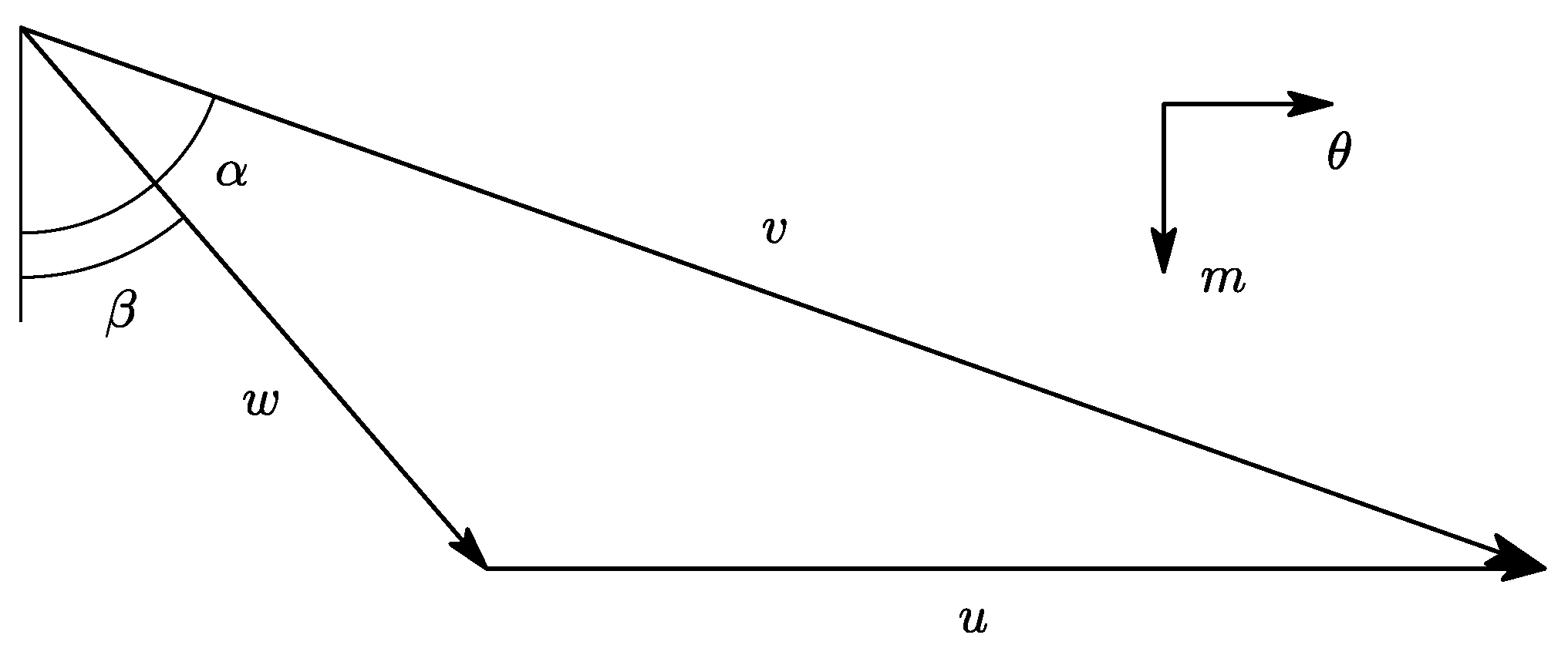
In this work the symbol v is used for the absolute velocity, w for the relative velocity, and u for the blade velocity. The components of velocity in the tangential and meridional directions are denoted with the subscripts and m, respectively. For the case of axial turbines, the meridional direction coincides with the axial direction. Regarding the sign convention for the velocity components, the positive axial direction is taken along the shaft axis from the inlet of the turbine to the outlet and the positive radial direction is taken as the turbine radius increases. The positive circumferential direction is taken in the direction of the blade speed.
The symbol
is used to denote the absolute flow angle while
is used for the relative flow angle. As shown in the velocity triangle of
Figure 2, all angles are measured from the meridional towards the tangential direction. This is the usual convention in the gas turbine industry and it bounds the flow angles to the interval
[
1] (p. 316). The advantage of this angle convention is that it is possible to use single-input inverse trigonometric functions directly. In addition, the same sign convention is used for stator and rotor blades for the sake of consistency. However, the loss model that is used in this paper [
23] employs a different sign convention for stator and rotor blades and some of the formulas of the loss model had to be adapted, see
Appendix A.
2.3. Design Specifications
A turbine is a component of a larger system that will impose some requirements on the turbine design, including: (1) stagnation state at the inlet of the turbine, (2) static pressure at the outlet of the turbine, and (3) mass flow rate. Alternatively, it is possible to specify the isentropic power output instead of the mass flow rate because both are related according to Equation (
1), where the subscripts 1 and 2 refer to the states at the inlet and outlet of the turbine, respectively, and the subscript
s refers to an isentropic expansion.
These design requirements can be regarded as the thermodynamic boundary conditions for the expansion and they are given inputs for the turbine model.
2.4. Cascade Model
This section describes the equations used to model the flow within stator and rotor cascades. All flow variables are evaluated at constant mean radius at the inlet and outlet of each cascade (mean-line model). The cascade model presented in this section is solved sequentially and it contains three blocks: (1) computation of the velocity triangles, (2) determination of the thermodynamic properties using the principle of conservation of rothalpy and equations of state, and (3) calculation of the cascade geometry.
2.4.1. Velocity Triangles
The equations used to compute the velocity diagrams for rotor and stator sections are the same, provided that the blade velocity is given by for the stators and for the rotors, where the angular speed and mean radius r are given as input variables.
The velocity triangles at the inlet of each cascade are computed according to Equations (2)–(7), where the subscripts that refer to inlet conditions have been dropped for simplicity. For the first stator, the absolute velocity
v and flow angle
are given as inputs. For the rest of cascades, the absolute velocity and flow angle are obtained from the outlet of the previous cascade.
The velocity triangles at the outlet of each cascade are computed according to Equations (8)–(13), where the subscripts that refer to outlet conditions have been dropped for simplicity. The relative velocity
w and flow angle
at the outlet of each cascade are provided as an input for the model.
2.4.2. Thermodynamic Properties
The axial turbine model was formulated in a general way and the thermodynamic properties of the working fluid can be computed with any set of equations of state that supports enthalpy–entropy function calls. In this work, the REFPROP fluid library was used for the computation of thermodynamic and transport properties [
24].
The stagnation state at the inlet of the first stator (for instance temperature and pressure) is an input for the model and the corresponding static state is determined according to Equations (14) and (15). The remaining static properties at the inlet of the first stator are determined with enthalpy–entropy function calls to the REFPROP library, see Equation (16). The static thermodynamic properties at the inlet of all the other cascade are obtained from the outlet of the previous cascade.
The thermodynamic properties at the outlet of each cascade are computed using the fact that rothalpy is conserved both in rotor and stator cascades [
9] (pp. 10–11). For purely axial turbines (constant mean radius), the conservation of rothalpy is reduced to the conservation of relative stagnation enthalpy, and the static enthalpy at the outlet of each cascade can be computed according to Equation (
17). In addition, the entropy at the outlet of each cascade is provided as an input to the model. Therefore, any other static thermodynamic property can be determined with enthalpy–entropy function calls to the REFPROP library, Equation (18).
2.4.3. Cascade Geometry
The geometry of the annulus is obtained from the principle of conservation of mass and geometric relations, Equations (
19)–(
23), where the mass flow rate
is given as an input for the model. These equations are valid both for the inlet and outlet of the cascade and the subscripts were not included for simplicity.
The mean blade height of the cascade is determined as the arithmetic mean of the blade height at the inlet and outlet of the cascade,
The blade chord is determined from the blade aspect ratio (input variable) and the mean blade height using Equation (
25). Similarly, the blade pitch (also known as spacing) is determined from the pitch to chord ratio (input variable) and the blade chord according to Equation (26).
The incidence
i and deviation
angles are assumed to be zero and, therefore, the metal angle at the inlet and outlet of each cascade are given by Equations (
27) and (
28), respectively.
The blade opening is given by Equation (
29). This equation is an approximation that neglects the effect or the curvature of the blade suction surface [
1] (pp. 343–344).
The maximum blade thickness is computed according to the formula proposed by Kacker and Okapuu [
23] that correlates the blade maximum thickness to chord ratio with the camber angle as given by Equation (
30). The blade camber angle is defined as
.
The stagger angle is computed according to Equation (
31), which assumes that circular-arc blades are used, Dixon and Hall [
9] (p. 72). Alternatively, the stagger angle could be computed using the graphical relation proposed by Kacker and Okapuu [
23] or given as an input for the model. The axial chord of the blades is determined using the geometric relation given by Equation (32).
The axial chord and blade height difference between inlet and outlet are used to compute the flaring angle of the cascade according to Equation (
33).
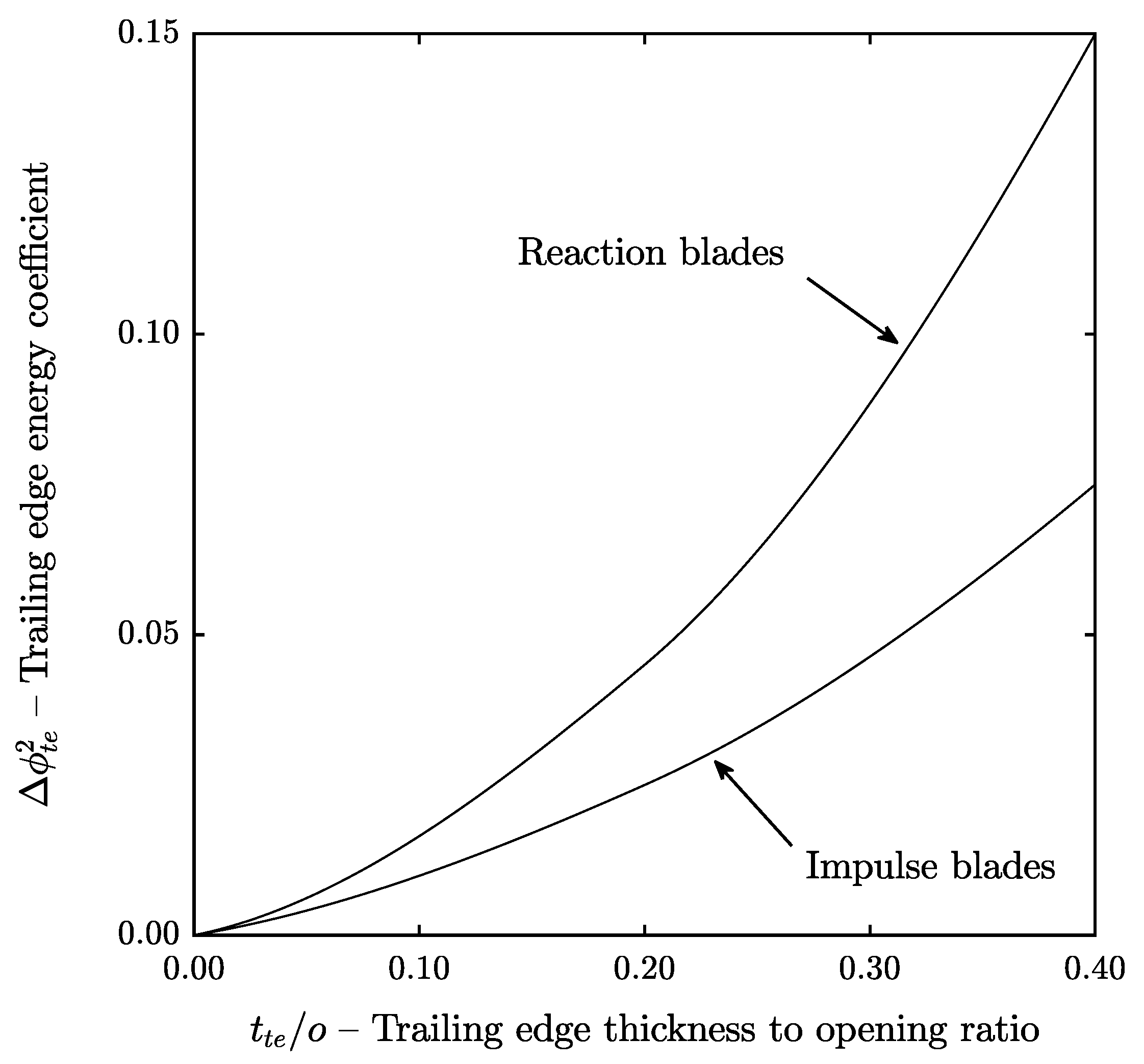
The trailing edge thickness is computed using the trailing edge thickness to opening ratio (input variable) and the cascade opening according to Equation (
34).
In addition, the axial spacing between cascades
can be computed as fraction of the axial chord. However, this variable does not affect the performance predicted by the model because the Kacker and Okapuu [
23] loss correlations neglect the influence of this parameter. Saravanamuttoo et al. [
1] (pp. 332–333) suggests that axial spacing to chord ratios between 0.20 and 0.50 are satisfactory. Finally, the tip clearance height of the rotor blades
is given as a fixed input to the model that depends on manufacturing limits. The geometry relations presented in this section allow a description of the turbine geometry in a level of detail that is adequate for preliminary design purposes. A more detailed design of the turbine geometry, such as the definition of the shape of the blades, requires more advanced mathematical models based on the fluid dynamics within the turbine rather than the algebraic loss models used in this work.
2.5. Loss Model
During the preliminary design phase, it is common to use empirical correlations to estimate the losses within the turbine. These sets of empirical correlations are known as loss models. Losses can be interpreted as any mechanism that leads to entropy generation within the turbine (which in turn reduces the power output), such as viscous friction in boundary layers or shock waves. See the work by Denton [
25] for a detailed description of loss mechanisms in turbomachinery.
Perhaps, the most popular loss model for axial turbines is the one proposed by Ainley and Mathieson [
26,
27] and its subsequent refinements by Dunham and Came [
28] and Kacker and Okapuu [
23]. The Kacker–Okapuu loss model has been further refined to account for off-design performance by Moustapha et al. [
29] and by Benner et al. [
30]. One of the remarkable aspects of the Ainley–Mathieson family of loss methods is that it has been updated with new experimental data several times since the first version of the method was published. This was not the case for other loss prediction methods such as the ones proposed by Balje and Binsley [
31], Craig and Cox [
32], Traupel [
33], or Aungier [
34]. A comprehensive review of different loss models is given by Wei [
35].
In this work, the Kacker and Okapuu [
23] loss model was selected because of its popularity and maturity. The improvements of this loss model to account for off-design performance were not considered because the axial turbine methodology proposed in this paper is meant for the optimization of design performance. The Kacker–Okapuu loss model is described in detail in
Appendix A. The formulation of the loss model has been adapted to the nomenclature and sign conventions used in this work for the convenience of the reader.
As described by Denton [
25] and by Dahlquist [
36], there are several definitions for the loss coefficient. In this work, the stagnation pressure loss coefficient was used because the Kacker–Okapuu loss model was developed using this definition. This loss coefficient is meaningful for cascades with a constant mean radius and it is defined as the ratio of relative stagnation pressure drop across the cascade to relative dynamic pressure at the outlet of the cascade, Equation (
35). This definition is valid for both rotor and stator cascades.
In general, the loss coefficient computed from its definition, Equation (
35), and the loss coefficient computed using the loss model,
Appendix A, will not match for an arbitrary set of input parameters. In
Section 4, the turbine design is formulated as an optimization problem that uses equality constraints to ensure that the value of both loss coefficients matches for each cascade. The loss coefficient error is given by Equation (
36).
2.6. Diffuser Model
The diffuser model is based on the transport equations for mass, meridional and tangential momentum, and energy in an annular channel. It assumes that the flow is one-dimensional (in the meridional direction), steady (no time variation), and axisymmetric (no tangential variation). The model can use arbitrary equations of state and it accounts for effects of area change, heat transfer, and friction. Under these conditions, the governing equations of the flow are given by Equations (37)–(40). The detailed derivation of these equations and a discussion of the physical meaning of the different terms is presented in the Appendix of Agromayor et al. [
10].
The viscous term is modeled using a constant skin friction coefficient
such that
and heat transfer is neglected,
. The geometry of the diffuser was modeled in a simple way assuming that the inner and outer surfaces are straight, see
Figure 1d. For this particular geometry, the diffuser channel height
and mean radius
are given by Equations (41) and (42), where the mean cant angle
and divergence semi-angle
are given as input parameters.
The initial conditions required to integrate the system of ordinary differential equations (ODE) are prescribed assuming that the thermodynamic state and velocity vector do not change from the turbine outlet to the diffuser inlet. The integration starts from the initial conditions and stops when the prescribed value of outlet to inlet area ratio
is reached. In this work, the MATLAB function
ode45 was used to perform the numerical integration [
37]. This function uses an automatic-stepsize-control solver that combines fourth and fifth order Runge–Kutta methods to control the error of the solution.
In general, the static pressure that is given as a design specification from a system analysis will not match the pressure at the outlet of the diffuser computed by the model. In
Section 4, the turbine design is formulated as an optimization problem that uses an equality constrain to ensure that the static pressure at the outlet of the diffuser and the target pressure match. The dimensionless outlet static pressure error is given by Equation (
43).
3. Validation of the Axial Turbine Model
The aim of this section is to validate the axial turbine model presented in
Section 2 using the experimental data of the one- and two-stage turbines reported by Kofskey and Nusbaum [
38]. The flow in both turbines is subsonic and they use air as working fluid. To validate the model, the geometry and operating conditions reported by Kofskey and Nusbaum [
38] were replicated and the design-point performance of both test cases was compared with the output of the model, see
Table 2. The inlet thermodynamic state, angular speed, and total-to-static pressure ratio were matched at the design point and the validation was performed analyzing the deviation in mass flow rate, power output, and total-to-static isentropic efficiency. This approach is consistent with the definition of the design point given by Kofskey and Nusbaum [
38]. The data reported in
Table 2 shows that the agreement between the predicted and measured mass flow rates and power outputs is satisfactory and that the relative deviation is less than 1.2% for both turbines. In addition, the deviation of total-to-static isentropic efficiency between model and experiment is 1.15 percentage points for the one-stage turbine and 0.60 points for the two-stage turbine, which is within the efficiency-prediction uncertainty of the loss model of
percentage points [
23]. The turbines reported in [
38] did not have a diffuser to recover the exhaust kinetic energy and therefore could not be used to validate the diffuser model. Nevertheless, the diffuser model used in this work has been validated in a previous publication [
10].
The analysis presented in this section showed that the axial turbine model can be used to predict the design-point performance of turbines with one or more stages. However, the validation was restricted to subsonic turbines using air as working fluid and it is likely that the efficiency predictions will not be as accurate for turbines with transonic–supersonic cascades or when the fluid behavior deviates from ideal gas, such as in Rankine cycles using organic fluids with high molecular mass or in supercritical carbon dioxide power systems.
5. Optimization of a Case Study
The aim of this section is to assess the optimization methodology proposed in this work. To do this, the model was tested against two reference axial turbine optimization problems presented in Macchi and Astolfi [
41]. The two cases consider pentaflueroethane (R125) expanding from 155 °C and 36.2 bar (stagnation properties) to 15.85 bar (static pressure). The mass flow rate is selected to achieve an isentropic power of 250 kW in the first case and 5000 kW in the second case. These two case studies are representative of a small-scale and a large-scale Rankine cycles used to generate power from a low-temperature heat source as in a geothermal, solar, biomass, or waste heat recovery application [
5].
The values of the fixed parameters, bounds of the optimization variables, and the nonlinear constrains used to formulate the optimization problem are summarized in
Table 3. The minimum hub-to-tip ratio constraint is always active at the exit of the last rotor, see
Section 6.3, and it has a great influence on the optimal angular speed and diameter. For this reason, the comparison of optimal speed and diameter will only be fair if the minimum hub-to-tip ratio is the same as in the reference case. The value
reported in
Table 3 is the same value used by Macchi and Astolfi [
41] (the minimum-hub-to tip ratio used by Macchi and Astolfi was not reported in the original publication, but it was confirmed by M. Astolfi in a personal communication).
The results of the optimization for the two cases considered are shown in
Table 4. It can be observed that the optimal angular speed and diameter of the reference case agree well with the results obtained with the turbine model presented in this work and that the maximum relative deviation is less than
. In addition, the model presented in this work captures the trend of the angular speed and diameter as the power output changes. The values of total-to-static efficiency from the reference case and the ones obtained in the present work are comparable although there are is a difference of 2.07 and 0.83 percentage points in the small-scale and large-scale cases, respectively. This difference is not surprising considering that the Craig and Cox [
32] loss model was used in the reference case while the Kacker and Okapuu [
23] model was used in the present work and that the efficiency-prediction uncertainty of these empirical loss models is approximately
percentage points, if not higher [
23].
6. Sensitivity Analysis
This section contains a sensitivity analysis of the 5000 kW reference case analyzed in the previous section to gain insight about the impact of several input parameters on turbine performance. The next subsections investigate the influence of: (1) isentropic power output, (2) tip clearance height, (3) minimum hub-to-tip ratio, (4) diffuser area ratio, (5) diffuser skin friction coefficient, (6) total-to-static pressure ratio, (7) number of stages and (8) angular speed and mean diameter on the total-to-static isentropic efficiency. Each of the analyses of this section studies the influence of these variables on the optimal solution while all other fixed parameters are the same as in the 5000 kW reference case summarized in
Table 3. The ranges of the variables were selected to cover a wide span of flow conditions and they are justified in each subsection. Other variables were not considered for the sensitivity analysis because they have a secondary influence on turbine performance or because they are inactive constraints.
6.1. Influence of Isentropic Power
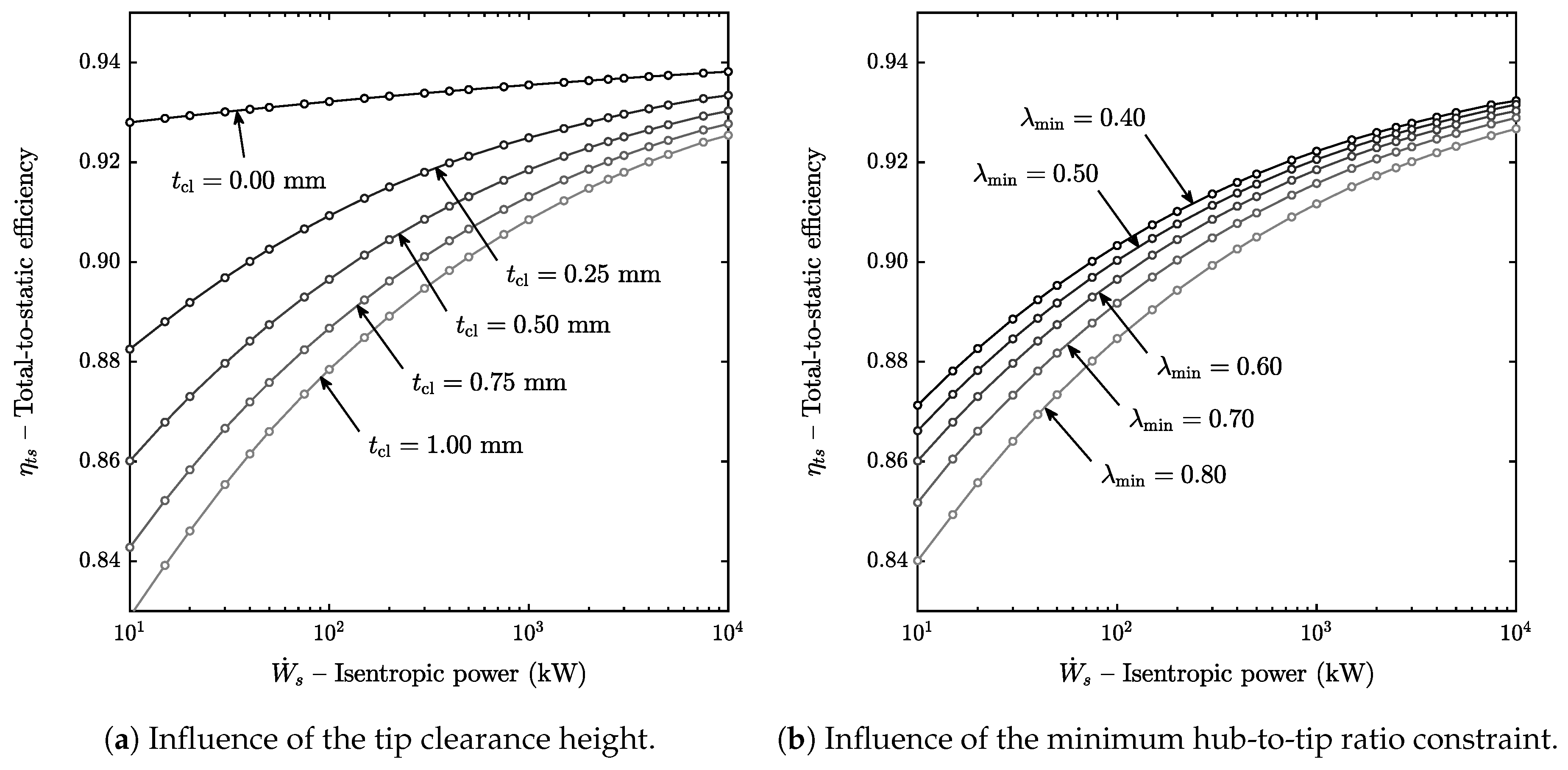
The isentropic power output was varied from 10 kW to 10 MW and the maximum attainable total-to-static efficiency is shown in
Figure 4a,b. This range of power output was selected to cover a wide spectrum of turbine scales. According to the classification for Rankine power systems using organics working fluids proposed by Colonna et al. [
5], this range of power output covers the mini, small, medium, and large power capacities.
It can be observed that the efficiency increases monotonously with the isentropic power and that the effect is more marked when the power output is small. The reason for this is that the size of the turbine increases and therefore: (1) the blade height
H increases and the
ratio decreases, which in turn reduces the tip clearance loss coefficient, see Equation (
A19), and (2) the blade chord of the cascades increases, which in turn increases the Reynolds number and reduces the profile loss coefficient, see Equation (
A1).
6.2. Influence of Tip Clearance
Figure 4a shows the total-to-static efficiency as a function of the isentropic power when the tip clearance height is varied from 0.00 mm (no clearance) to 1.00 mm (high clearance). It can be observed that the isentropic efficiency decreases when the tip clearance is increased and that the trend is not linear. For instance, increasing the tip clearance from 0.00 mm to 0.25 mm penalizes the efficiency more than from 0.25 to 0.50 mm.
It can also be seen that the efficiency drop due to tip clearance is more marked when the isentropic power is low because the ratio is increased both due to blade height reduction and tip clearance increase. In addition, note that total-to-static efficiency increases with the isentropic power output even for the case when the rotor tip clearance is zero due to Reynolds number effects.
6.3. Influence of the Hub-to-Tip Ratio
The influence of the lower limit for the hub-to-tip ratio constraint on the turbine performance as a function of the isentropic power is shown in
Figure 4b, where the low value
is representative of low-pressure steam turbine stages and the high value
is representative of gas turbines or high-pressure steam turbine stages. The results of the optimization showed that the constraint for the minimum hub-to-tip ratio is always active at the outlet of the turbine, i.e., the turbine model proposed in this work predicts that the isentropic efficiency will always increase when the allowable lower limit for the hub-to-tip ratio is decreased.
The reason for this is that the blade height is increased when the minimum hub-to-tip ratio decreases and, as a result of this, (1) the tip clearance to blade height ratio
and the clearance loss coefficient decrease and (2) for a fixed aspect ratio, the blade chord and Reynolds number increase and the profile loss coefficient is reduced. In addition, the channel height of the diffuser increases according to
, see
Figure 1d. This in turn reduces the friction losses in the diffuser because the channel height appears in the denominator of the friction terms of the diffuser model, Equations (38)–(40). The effect of the hub-to-tip ratio on the friction losses of the diffuser agrees with the results obtained by the authors in a previous work [
10], but its impact on the isentropic efficiency is marginal compared with the impact of profile and tip clearance losses.
6.4. Influence of the Diffuser Area Ratio
The effect of the diffuser area ratio on the total-to-static isentropic efficiency is shown in
Figure 5a,b. The limits of the area ratio were selected to include cases ranging from the absence of diffuser
, to cases where a large fraction of the kinetic energy is recovered
. This upper limit was selected because, for the case of inviscid, incompressible flow with no inlet swirl, a diffuser with an area ratio of
would recover 96% of the available dynamic pressure [
10].
Both
Figure 5a,b show that the isentropic total-to-static efficiency increases with the area ratio in an asymptotic way. A small increase of area ratio from the case with no diffuser
increases the total-to-static efficiency significantly, whereas, as the area ratio is higher, the improvement of isentropic efficiency becomes less marked because there is less kinetic energy to recover at the diffuser exit. The results of the optimization showed that using an area ratio in the range 2.0–2.5 achieves 70–80% of the maximum efficiency gain. In addition, it was found that the optimum absolute flow angle at the outlet of the last rotor was very close to zero (no swirl) for all cases, regardless of the area ratio of the diffuser.
6.5. Influence of the Skin Friction Coefficient
To the knowledge of the authors, there are no correlations available to predict the skin friction coefficient for annular channels with swirling flow. However, it is possible to estimate a reasonable value for the skin friction coefficient based on experimental data from vaneless diffusers without flow separation. Brown [
42] measured the local skin friction coefficient for different vaneless diffusers and obtained values in the range 0.003–0.010. In the absence of better estimates, Johnston and Dean [
43] recommend values within the range 0.005–0.010 for the global skin friction coefficient. In a similar way, Dubitsky and Japikse [
44] suggest 0.010 as a reasonable estimate for the global skin friction coefficient, but noted that values from 0.005 to 0.020 were required to fit experimental data, depending on the application.
In this section, the friction factor was varied from 0.000 (frictionless) to 0.030 (high friction) and the impact on the turbine total-to-static isentropic efficiency is shown in
Figure 5a as a function of the area ratio. This range of skin friction factor is representative of well-designed diffusers with attached boundary layers. If the adverse pressure gradient is too high and causes flow separation, the friction losses in the diffuser would increase significantly reducing the pressure recovery and the turbine total-to-static isentropic efficiency [
45].
It can be observed that increasing the friction factor decreases the total-to-static isentropic efficiency in a linear way (the different curves are equispaced). In addition, the impact of friction factor on the efficiency drop is more notable as the area ratio is high because the length of the channel increases. However, the effect of the friction factor has only a modest impact on the total-to-static efficiency as it causes an efficiency drop of ∼0.3 percentage points for the worst case of
Figure 5a.
6.6. Influence of the Total-to-Static Pressure Ratio
The effect of the pressure ratio as a function of the diffuser area ratio is shown in
Figure 5b. The pressure at the outlet of the turbine was kept constant and the pressure at the inlet was varied to achieve pressure ratios ranging from
(subsonic flow) to
. It can be observed that increasing the pressure ratio from
to
causes a small efficiency drop and that further increasing the pressure ratio to
causes a much larger efficiency drop. The reason for this is that the Mach number at the outlet of the cascades becomes higher than unity when
and the supersonic correction factor of the Kacker and Okapuu [
23] loss system, see Equation (
A4), penalizes the total-to-static isentropic efficiency.
In addition,
Figure 5b also shows that the total-to-static isentropic efficiency of turbines without diffuser deteriorates rapidly when the pressure ratio is increased. This is because increasing the turbine pressure ratio increases the flow velocities within the turbine and the amount of kinetic energy that is potentially wasted at the outlet. This highlights the importance of using a diffuser when the pressure ratio is high.
6.7. Influence of the Number of Stages
Figure 6 shows the total-to-static efficiency of turbines with one, two, and three stages as a function of the pressure ratio. Again, the pressure ratio was achieved varying the pressure at the inlet of the turbine while keeping the outlet pressure constant. However, in this case, the upper limit of the pressure ratio increased to
.
In can be seen that there is a peak of efficiency and that the performance deteriorates rapidly when the pressure ratio increases beyond this point because the flow becomes supersonic and the Mach number correction factor penalizes the profile loss coefficient, see Equation (
A4). Moreover, the range of pressure ratios for which the isentropic efficiency is high becomes wider as the number of stages increase because the expansion can be distributed over more cascades and the number of optimization variables increases.
6.8. Influence of the Angular Speed and Diameter
The results presented in the previous subsections correspond to the optimal values of angular speed and diameter because the specific speed and specific diameter were independent optimization variables with inactive upper and lower bounds. Depending on the application, it might not be possible to achieve the point of optimal angular speed and diameter because of technical constraints that were not considered in the analysis such as the frequency of the electrical grid, mechanical stress, or space limitations. The objective of this section is to analyze the impact of using a non-optimal angular speed and diameter on the total-to-static efficiency of the turbine. To make the conclusions general, the analysis is presented in terms of dimensionless variables.
Figure 7 shows the contours of maximum total-to-static isentropic efficiency in the
-
plane for the 5000 kW reference case of
Table 3. In this diagram, often referred as Baljé diagram, the specific speed and specific diameter are regarded as fixed parameters while the rest of the independent optimization variables are free. It can be observed that there exist an optimum specific speed and specific diameter that maximize the total-to-static isentropic efficiency. In addition, there is a narrow region where the efficiency is close to its maximum value and that moving away from this region leads to a rapid decrease in efficiency. Interestingly, the loci of maximum efficiencies are approximately given by the hyperbola of Equation (
50).
This suggests that the efficiency penalty away from the point of optimal specific speed and specific diameter is small if the dimensionless blade velocity
is close to unity. This simple result can be explained from Euler’s turbomachinery equation and the behavior of the solutions that maximize efficiency. On the one hand, close-to-optimal solutions tend to minimize the swirling kinetic energy lost at the exit of the turbine, see
Section 6.4. As a consequence, the absolute flow angle and tangential velocity at the rotor exit are close to zero (
and
). On the other hand, close-to-optimal solutions also tend to have a relative flow angle at the inlet of the rotor that is close to zero (
) because the Kacker and Okapuu [
23] loss system predicts low profile losses for reaction blades with small relative inlet angles, see Equation (
A7). As a result, of this, the absolute tangential velocity at the inlet of the rotor approaches the blade velocity (
).
Under these conditions, the actual enthalpy change approaches the isentropic enthalpy change (
) and Euler’s turbomachinery equation, Equation (
51), is reduced to Equation (52), which corresponds to the hyperbola of maximum efficiencies in the Baljé diagram.
This analysis was valid for single-stage turbines, but it can be extended to turbines with more than one stage. For the case of a multistage turbine, it was observed that the loci of maximum efficiencies are approximately given by the hyperbola of Equation (
53). This relation can also be explained from Euler’s turbomachinery when
and
hold for every stage.
To assess the validity of this result, the optimal blade speed predicted by Equation (
53) was compared with the results of numerical optimization for different isentropic power outputs ranging between 10 kW and 10 MW and different pressure ratios ranging between 2 and 14, see
Table 5. It can be observed that location of the point of maximum efficiency predicted by Equation (
53) agrees well (relative deviation <4%) with the optimization results for axial turbines of 1, 2, and 3 stages regardless of the pressure ratio and the isentropic power output.
7. Conclusions
A mean-line model and optimization methodology for axial turbines with any number of stages was proposed. The model was formulated to use arbitrary equations of state and empirical loss models and it accounts for the influence of the diffuser on turbine performance using a one-dimensional flow model proposed by the authors in a previous publication [
10]. To the knowledge of the authors, this was the first time that a diffuser model has been coupled with a mean-line model for the optimization of axial turbines. The axial turbine preliminary design was formulated as a constrained optimization problem and was solved using a sequential quadratic programming algorithm. Employing a gradient-based algorithm (instead of a direct search one) allowed to use equality constraints to integrate the cascade, loss, and diffuser sub-models in a simple way.
The model was validated against two test cases from the literature and it was found that the deviation between experimental data and model prediction in terms of mass flow rate and power output was less than 2.5% for both cases and that the deviation in total-to-static efficiency was only 0.27 percentage points for the one-stage case and 0.35 points for the two-stage case. It was also concluded that the close match between measured and predicted efficiencies is probably incidental because the uncertainty of the efficiencies predicted by the loss model is approximately percentage points. In addition, the optimization methodology was applied to a case study from the literature and a sensitivity analysis was performed to investigate the influence of several design variables on the total-to-static isentropic efficiency, gathering the following conclusions and design guidelines:
The total-to-static isentropic efficiency increases when the tip clearance height decreases, and this effect is more marked as the isentropic power output of the turbine decreases. This highlights the importance of using small tip clearances in small-scale applications.
The total-to-static isentropic efficiency increases when the minimum hub-to-tip ratio constraint is reduced (this constraint is always active at the exit of the last rotor). However, reducing the minimum hub-to-tip ratio also increases the centrifugal and gas bending stresses [
1]. Therefore, the choice of minimum hub-to-tip ratio must be a trade-off between the fluid-dynamic and the mechanical designs.
The total-to-static isentropic efficiency increases with the diffuser area ratio in an asymptotic way, regardless of the value of the diffuser skin friction coefficient, and the results of the optimization showed that using an area ratio in the range 2.0–2.5 achieves 70–80% of the maximum efficiency gain. Using a higher diffuser area ratio will increase the kinetic energy recovery and the power output; but it will also increase the turbine footprint, which may be a disadvantage for applications with space limitations.
The total-to-static isentropic efficiency decreases when the pressure ratio is increased beyond a certain value because the Kacker and Okapuu [
23] loss model predicts an increase of the profile loss coefficient when the flow becomes supersonic. This effect becomes less marked as the number of stages increases because the expansion can be distributed over more cascades. In addition, the total-to-static efficiency of turbines without diffuser deteriorates rapidly when the pressure ratio is increased, highlighting the importance of using a diffuser when the pressure ratio is high.
The results of the optimization showed that the maximum total-to-static isentropic efficiency is attained when the absolute flow angle at the exit of the last stage is close to zero (no exit swirl), regardless of the area ratio of the diffuser. This agrees with the conclusions drawn in a previous work from the authors where the flow within the diffuser was examined in more detail [
10].
It was found that the efficiency penalty away from the point of optimal angular speed and diameter, peak of the Baljé diagram, is small if the combination of specific speed and diameter is close to the hyperbola given by . This guideline can be used to select a suitable combination of angular speed and diameter when one of these variables is imposed by technical constraints such as the frequency of the electrical grid, mechanical stress, or space limitations.


