Article

Verification of the Axial Momentum Theory for Propellers with a Uniform Load Distribution †

Dipartimento di Ingegneria Industriale, Università degli Studi di Napoli Federico II, via Cluadio, 21, 80125 Napoli, Italy
*
Author to whom correspondence should be addressed.
This paper is an extended version of our paper published in the Proceedings of the 13th European Conference on Turbomachinery Fluid Dynamics and Thermodynamics.
Int. J. Turbomach. Propuls. Power 2019, 4(2), 8; https://doi.org/10.3390/ijtpp4020008
Submission received: 18 April 2019 / Revised: 8 May 2019 / Accepted: 8 May 2019 / Published: 14 May 2019

Abstract

:
The paper provides an evaluation of the errors embodied in the Axial Momentum Theory (AMT) as applied to a uniformly loaded actuator disk model without wake rotation. Although this model exhibits some unphysical features, such as the tip singularity and the violation of the angular momentum equation, it is still considered a touchstone in the theoretical aerodynamics of propellers. To simplify the model, a purely mathematical assumption is commonly used in the differential form of the axial momentum equation, i.e., the contribution of the pressure forces on the lateral surface of the infinitesimal streamtubes swallowed by the disk is neglected. In this paper, the errors introduced by this simplifying assumption are evaluated by comparing the results of the AMT with those of a nonlinear method modelling the free wake as the superposition of ring vortices distributed along the wake boundary. Firstly, the validity of this method is verified in terms of global performance coefficients. Then, using a CFD approach, it is also verified in terms of local flow quantities. The comparison between the ring-vortices method and the AMT shows that, for a highly loaded propeller, significant errors exist in the axial velocity at the disk, especially near the tip. Moreover, despite the uniform load, the axial velocity at the disk varies in the radial direction. Instead, the velocity magnitude remains almost uniform only for values of the thrust coefficient lower than 1.

1. Introduction

Not disregarding the classical CFD approaches [1,2,3,4,5,6], the design and/or analysis of aeronautical and marine propellers are generally carried out using many numerical methods such as lifting-line [7,8], lifting surface [9,10] and panel methods [11,12]. However, when compared with the classical engineering approach based on the momentum theory, these models have never shown a definitive improvement in the accuracy of the performance prediction and/or in the robustness of the numerical algorithm [13]. For this reason, despite the great variety of more advanced methods, the simple and robust Blade-Element Momentum Theory is still the most used approach for the evaluation of propeller performance. This theory stems from the coupling of the Blade-Element Theory and of the Momentum Theory (MT). Two versions of this latter theory exist: the generalized (GMT) and the axial (AMT) Momentum Theory [14]. While the former takes into account the wake rotation, the AMT completely disregards the tangential velocity, even in the wake. The MT relies on the steady, incompressible, axisymmetric, and inviscid flow assumptions. However, additional simplifying assumptions are typically introduced when the MT is used to evaluate local quantities such as the radial distribution of the axial velocity at the disk. Specifically, as shown in [15,16,17,18,19], the AMT disregards the axial contribution of the pressure forces on the lateral surfaces of the infinitesimal streamtubes swallowed by the rotor. Due to the great relevance of this theory, the evaluation of its errors and the impact on the reliability of its results are of interest. Generally, the evaluation of these errors is carried out by comparing the MT results with those of more advanced actuator disk approaches which do not rely on the MT simplifying assumptions. For example, consider the nonlinear actuator disk of Wu [20] further developed in [21,22,23]. The method has been also extended to a ducted configuration in [24,25,26,27,28,29,30]. The ring-vortex wake method proposed by Øye [31] has also been employed by van Kuik and Lignarolo [32] to verify the AMT when applied to a wind turbine. Sørensen and Mikkelsen [33], Madsen et al. [34], Sørensen [35] and Madsen et al. [36] also assessed the validity of the MT using several actuator disk approaches.
Despite the large amount of works on this topic, a precise evaluation of the AMT errors as applied to the classical uniformly loaded propeller is still missing. The relevance of this issue relies on the fact that the uniformly loaded disk still represents the benchmark model for two reasons. Firstly, thanks to its great simplicity, this model is the most studied and used approach. Secondly, it can be easily proven that a uniformly loaded disk is characterized by the maximum propulsive efficiency, thus making this oversimplified model a reference point for the performance estimation of real propellers. In this paper, the errors embodied in the AMT as applied to a uniformly loaded propeller are evaluated comparing its results with those of a free-wake ring-vortex actuator disk (FWRV-AD) method which models the wake through the superposition of ring vortices placed in the control points of N straight panels [37,38]. The far wake is represented by a semi-infinite vortex cylinder. The velocity induced by a panel on itself is computed considering the wake curvature both in the cross and meridional plane. Two constrains are used to iteratively evaluate the wake shape and the density strengths of the vortices, i.e., the panels are required to be aligned with the overall flow field and to have a zero static pressure jump across them.
The article is organized as follows. Firstly, the typical simplifying assumptions used in the AMT are described in Section 2. Then, most of the theoretical and numerical aspects of the FWRV-AD method are outlined, and its stability and convergence properties are discussed in some details (see Section 3). Moreover, its results are verified in terms of global performance coefficients using the AMT in Section 4.1. A further verification in terms of local flow quantities is carried out against a CFD actuator disk model (see Section 4.2). Finally, in Section 4.3, the AMT errors on the axial velocity at the disk, and on the axial induction factor are quantified.

2. The Axial Momentum Theory for the Uniformly Loaded Propeller: Review and Analysis of the Simplifying Assumptions

In the AMT, a uniformly loaded propeller is modelled by the steady, incompressible, inviscid, and axisymmetric flow through an actuator disk which experiences a uniform pressure jump across it. To fully take advantage of the axisymmetric flow assumption, a cylindrical coordinate system (z, r, θ ) is introduced. The z axis is orthogonal to the disk face and, by convention, oriented in the downstream direction. Without loss of generality, the origin of the reference frame is placed at the disk center. Moreover, to further simplify the analysis, the tangential velocity is typically assumed to be zero everywhere, even in the wake. Obviously, for finite rotor angular velocity, this assumption contradicts the angular momentum equation. However, since the dynamic load associated with the change in the tangential velocity is usually small in comparison with the static load, the above assumption is generally accepted as a first approximation. Moreover, it can be easily proven [15] that a uniformly loaded actuator disk without wake rotation is characterized by the maximum propulsive efficiency, thus making this oversimplified model a reference point for the performance of real propellers.
At upstream infinity, the axial velocity v z ( z , r ) and the static pressure p ( z , r ) are considered to be uniform and, for the sake of simplicity, they are termed v and p , respectively. Across the disk, the axial v z ( 0 , r ) and the radial v r ( 0 , r ) velocity are supposed to be continuous (that is v z ( 0 , r ) = v z ( 0 + , r ) and v r ( 0 , r ) = v r ( 0 + , r ) ). The axial and radial velocities at the disk are termed v z , d and v r , d , where the subscript d stands for disk. While the velocity components are continuous functions across the disk, a radially uniform pressure jump Δ p d takes place there, i.e., Δ p d = p ( 0 + , r ) p ( 0 , r ) = c o n s t . At downstream infinity, the wake is supposed to be fully developed in the axial direction without a radial velocity component. Then, since there is no rotation in the wake, it is easy to show that the static pressure at downstream infinity is everywhere equal to p [15], a fact that can be easily proven using the Bernoulli and the radial momentum equations. The wake axial velocity at downstream infinity v z ( z + , r ) is termed v z , w . This quantity can be related to the pressure jump across the disk by applying the Bernoulli equation to the streamtubes swallowed by the rotor. By so doing, it can be shown that
Δ p d = 1 2 ρ ( v z , w 2 v 2 ) ,
where ρ is the fluid density. The above equation implies that if a uniform pressure jump exists all along the rotor span, then the wake axial velocity at downstream infinity v z , w must be uniform in the radial direction, too. Since Δ p d > 0 for a propeller, Equation (1) also means that the axial velocity in the wake must be greater than v , so that, using the continuity equation, the streamtube swallowed by the disk must contract moving from upstream to downstream infinity.
A further relation between the rotor load and the wake velocity can be obtained by applying the axial momentum equation which returns [15]
T = S Δ p d d S = 0 R ρ v z , d ( r ) v z , w r w ( r ) v 2 π r d r ,
where T is the propeller thrust and S = π R 2 is the rotor swept area. Moreover, if r is the radius of a generic streamtube at z = 0 , then the function r w ( r ) returns the radius of that streamtube at downstream infinity. When a uniform pressure jump is used, Equation (2) reduces to
Δ p d = ρ ( v z , w v ) v ¯ z , d .
In the above equation v ¯ z , d is the area averaged axial velocity at the disk defined as
v ¯ z , d = 1 π R 2 S v z ( 0 , r ) d S .
Then, from Equations (1) and (3), it is easy to prove that the averaged axial velocity at the disk is the arithmetic mean between the velocity at upstream and downstream infinity i.e.,
v ¯ z , d = v z , w + v 2 .
Under all the aforementioned simplifying assumptions, Equations (1)–(5) are exact. However, in the AMT, these equations are further simplified by adopting the following differential form of Equation (2):
Δ p d = ρ v z , d ( v z , w v )
which, making use of Equation (1), promptly returns the famous Froude law
v z , d AMT = v z , w + v 2 .
Contrarily to Equation (5), the above equation implies that for a uniform Δ p d , the axial velocity at the disk must be radially uniform, too. For this reason, the AMT is often considered a one-dimensional theory. However, as shown in [16,17,32,33], Equation (6), and so (7), are not exact since they disregard the effect of the pressure forces on the lateral surface of the infinitesimal streamtubes swallowed by the rotor. As discussed in [16], this effect is intimately related to the wake contraction. In Equation (7), the superscript AMT is used to denote the axial velocity at the disk evaluated under the simplifying assumptions of the AMT. Also note that Equations (5) and (7) readily yield v z , d AMT = v ¯ z , d .
In the following sections, it is shown that, even if the load is uniform, the flow through a uniformly loaded disk is not one-dimensional since the axial velocity at the disk is not uniform. Moreover, the errors introduced in Equations (6) and (7) are evaluated comparing them with the results of the FWRV-AD model which does not rely on the simplifying assumption used to retrieve those equations.

3. The Free-Wake Ring-Vortex Model for the Uniformly Loaded Propeller without Wake Rotation

The actuator disk method described in this section stems from an infinite-blade variant of the Joukowsky vortex model [
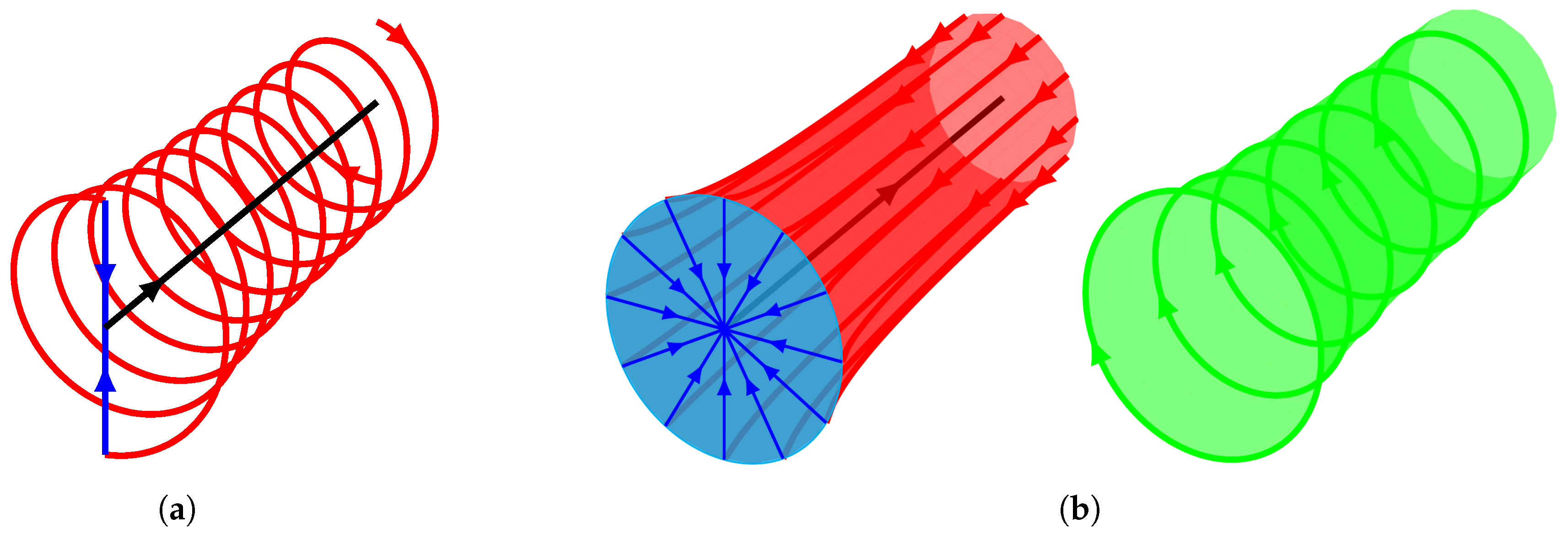
39]. Basing on the Stokes and Kutta-Joukowsky theorems, this model represents each blade as a line vortex. In fact, a lift force is typically related to each blade section which, using the Kutta-Joukowsky theorem, must experience a bound circulation, too. Hence, from the Stokes theorem, a non-zero vorticity flux exists through any surface containing the blade section. This justifies the modelling of the blades through vortex lines. When a variation of the lift force takes place along the blade span, the associated vorticity flux must change accordingly. Since the vorticity is a solenoidal vector field, a trailing vorticity is also associated with the bound circulation variation. However, for a rotor with a uniform lift force distribution, the trailing vorticity is spread only from the tip and the root of the blades. Summarizing, three vortex systems are used to model the rotor: the blade bound vorticity, a straight line vortex representing the vorticity originating by the roots of the blades, and helicoidal vortex filaments for the vorticity spread by the blade tips (see Figure 1a). This filament is customarily decomposed in a tangential and in a meridional wake vortex system [40].
In the limiting case of infinite blades, the two components of the wake vortex filaments are spread over the wake boundary-surface to obtain two contoured cylindrical sheet-vortices (see Figure 1b) whose strengths are directed in the meridional and tangential direction, respectively. The blade line-vortices are also uniformly distributed on the swept disk surface, while the root vortex is unchanged.
Please note that the tangential vorticity induces an axial and a radial velocity, whereas the meridional component of the vorticity can also induce a tangential velocity. Hence, to obtain the classical actuator disk without wake rotation by the Joukowsky model, the blade, the root, and the meridional wake vorticity must be neglected, while the sole tangential vortex-sheet of the wake has to be used.
The geometry and the strength distribution of this tangential vortex-sheet, which represents the boundary of the wake, are not known a priori, and they must be computed using two different conditions. Firstly, the sheet must be aligned with the overall flow field, a condition which allows evaluation of the wake geometry. Secondly, the stability of the wake edge has to be enforced by requiring that the static pressure just beneath and above the sheet is the same, i.e., Δ p s v = 0 , where the subscript s v stands for sheet vortex. By so doing, the strength distribution of the sheet vortex can be evaluated as described in the following. First, it is convenient to introduce a curvilinear abscissa s along the wake edge, with s = 0 at the rim of the disk. Then, a density strength distribution γ is also introduced along the sheet, so that the strength of a sheet-element with infinitesimal length d s becomes γ d s (see Figure 2).
By convention, γ is considered to be clockwise-positive around the positive z axis, and thus, from the Stokes theorem, the strength γ d s is equal to the clockwise velocity circulation around the dashed curve reported in Figure 2. Then, it is easy to prove that
γ = v s v + v s v ,
where v s v and v s v + are the velocities just beneath and above the sheet, respectively. Please note that since the velocity in a propeller wake is higher than that outside it ( v s v > v s v + ), γ is a negative quantity all along the wake.
To enforce the free-force condition Δ p s v = 0 on the wake edge, consider now the total pressure distribution inside and outside the wake. As stressed in the previous section, the axial and radial velocities are supposed to be continuous functions across the disk ( v z ( 0 , r ) = v z ( 0 + , r ) and v r ( 0 , r ) = v r ( 0 + , r ) ), whereas no tangential velocity exists both ahead and behind the disk. Then, the uniform pressure jump across the rotor plane is directly associated with a uniform total pressure jump there, namely
C T = ( p t , w p t , ) / ( 1 2 ρ v 2 ) ,
where C T = Δ p d / ( 1 2 ρ v 2 ) is the thrust coefficient, while p t , w and p t , are the uniform total pressure inside and outside the wake, respectively. The same total pressure jump also exists across the sheet vortex which actually separates the wake from the stream not swallowed by the rotor. Hence, the static pressure difference across the sheet readily reads Δ p s v = p t , p t , w + 1 / 2 ρ ( v s v 2 v s v + 2 ) . Consequently, the sheet stability condition Δ p s v = 0 returns p t , p t , w = 1 / 2 ρ ( v s v + v s v ) ( v s v + + v s v ) which, with the help of Equations (8) and (9), promptly becomes
C T = 2 γ ^ v ^ s v .
In the above equation, v s v is the velocity at the sheet defined as v s v = 1 / 2 ( v s v + + v s v ) , while γ ^ = γ / v and v ^ s v = v s v / v . Please note that hereafter the disk radius R and the freestream velocity v are used as reference in all dimensionless quantities. The free-force condition (10) implies that the product γ ^ v ^ s v must be uniform on the sheet vortex, and it can be used to evaluate the density strength along the wake edge once the sheet velocity distribution and the thrust coefficient are known. At downstream infinity, the stability condition (10) can be cast in a simplified form. Recall that as stressed in the previous section, the static pressure tends to p as z + . Thus, from Equation (9), the wake axial velocity at downstream infinity becomes
v ^ z , w = 1 + C T .
Glauert [15] showed that the axial velocity outside the wake must reach the freestream velocity v as z + . Therefore, at downstream infinity, the sheet velocity becomes v ^ s v , z + = ( 1 + 1 + C T ) / 2 , while the density strength reads
γ ^ z + = 1 1 + C T .

3.1. The Discrete Free-Wake Ring-Vortex Model

The tangential sheet vortex can be modelled as the superposition of ring vortices placed in the control points of N annular panels. Furthermore, a semi-infinite vortex cylinder (SIVC), aimed at modelling the fully developed far wake, is also introduced. Figure 3 shows a sketch of this model in the meridional view.
The diamonds represent the endpoints of the panels whose lengths are Δ s n with n = 1 , , N . Crosses are used to denote the control points of the panels where the anticlockwise ring vortices are located. The density strength of the n-th ring-vortex, with center at z n and radius r n , is γ n Δ s n , where γ n is obviously the unknown density strength. The SIVC begins at z SIVC , while R SIVC is the radius of this vortex element and γ SIVC is its density strength.
The overall velocity induced at the control point of the m-th panel can be expressed as the sum of four contributions, viz. the self-induced velocity by the m-th panel, the velocity induced by the other N 1 ring vortices, the one induced by the SIVC, and, finally, the free stream contribution. Thus, the axial and radial velocity components at the m-th panel can be written in dimensionless form as
v ^ z , m = n = 1 N v ^ z , n m + v ^ z , SIVC m + 1 and v ^ r , m = n = 1 N v ^ r , n m + v ^ r , SIVC m ,
respectively. In the above equation, v z , m is the overall axial velocity induced on the m-th panel, while v z , n m and v z , SIVC m are the axial velocities induced on the control point of the m-th panel by the n-th ring vortex and by the SIVC, respectively. A similar notation is used for the radial velocities. However, in order to use Equation (13), the velocities induced by a ring vortex and a SIVC must be evaluated. In the following, the expressions used to compute the velocity components induced by a ring vortex are first given. Then, the SIVC flow field is described.
Considering the generic point P with coordinates ( z P , r P ) , the axial and radial velocities induced by the n-th ring vortex at P can be cast in the following form [41]:
v ^ z , n P = γ ^ n Δ s ^ n 2 π r ^ n z ˜ 2 + ( r ˜ + 1 ) 2 K ( k ) 1 + 2 ( r ˜ 1 ) z ˜ 2 + ( r ˜ 1 ) 2 E ( k ) ,
v ^ r , n P = γ ^ n Δ s ^ n z ˜ / r ˜ 2 π r ^ n z ˜ 2 + ( r ˜ + 1 ) 2 K ( k ) 1 + 2 r ˜ z ˜ 2 + ( r ˜ 1 ) 2 E ( k ) ,
where z ˜ = ( z P z n ) / r n and r ˜ = r P / r n . As customary, K ( k ) and E ( k ) are used to denote the complete elliptic integrals of the first and second kind with modulus k = 4 r ˜ / [ z ˜ 2 + ( r ˜ + 1 ) 2 ] . For 0 k 1 , the value of these two special functions can be numerically computed using several approaches, viz. series expansions, integration-based methods, duplication techniques, look-up table, polynomial approximations etcetera. All these methods show some pros and contra. For example, series expansion approaches require a significant computational cost to obtain high accuracy, while the convergence rate of integration methods is quite slow moving towards the singular point k = 1 . For this reason, the more efficient Arithmetic-Geometric Mean method [42] is used in this work. 
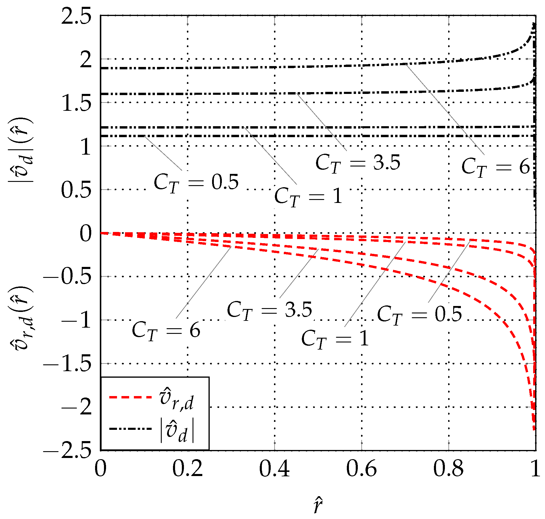
Figure 4a shows the streamlines of the flow induced by a unit strength ring vortex with center in z ^ = 0 and unity radius. This figure also clarifies the adopted convention for the sign of the ring-vortex strength. The radial profiles of the axial and radial velocity at different axial stations are reported in Figure 4b.
The self-induced velocity ( m = n ) of a rectilinear panel is evaluated following the approach proposed by Lewis [43]. The latter expressed the self-induced velocity as the sum of two contributions associated with the sheet curvature in the (r, θ ) and (z,r) planes, respectively. For the sake of simplicity, Lewis [43] assumed that both curvatures act independently and their contributions can be estimated separately. The contribution due to the curvature in the ( z , r ) plane is assumed to be equal to the self-induced velocity of a planar rectilinear panel; an assumption that returns a reasonable accuracy provided Δ s m / r m is small. The contribution associated with the ( r , θ ) curvature can be evaluated considering the approximate Lamb [44] formula for the self-induced velocity of a smoke ring vortex. Specifically, this contribution has been evaluated in [45,46] adapting the Lamb [44] expression to a ring surface vorticity element. Having said that, the axial and radial components of the overall self-induced velocity can be written as [43]
v ^ z , m m = β m + 1 β m 1 8 π cos β m Δ s ^ m 4 π r ^ m ln 8 π r ^ m Δ s ^ m 1 4 γ ^ m ,
v ^ r , m m = β m + 1 β m 1 8 π γ ^ m sin β m ,
where β is the slope of the panel.
The last vortex element to be analyzed is the SIVC. Its induced velocity can be retrieved by directly integrating the Biot-Savart law along the lateral surface of the cylinder [47]. By so doing, the axial and radial velocity components induced at P ( z P , r P ) read
v ^ z , SIVC P = γ ^ SIVC 2 π δ + z * z * 2 + ( r * + 1 ) 2 K ( k ) r * 1 r * + 1 Π ( n , k ) ,
v ^ r , SIVC P = 2 γ ^ SIVC π k 2 z * 2 + ( r * + 1 ) 2 E ( k ) 1 k 2 2 K ( k ) ,
where z * = ( z P z SIVC ) / R SIVC , r * = r P / R SIVC , δ = 0 for r * > 1 , δ = π / 2 for r * = 1 and δ = π for r * < 1 . Moreover, Π ( n , k ) is the complete elliptic integral of the third kind with modulus k = 4 r * / [ z * 2 + ( r * + 1 ) 2 ] and characteristic n = 4 r * / ( r * + 1 ) . This special function, which is evaluated using the duplication algorithm proposed in [48,49], exhibits a singular behavior when r * tends to the unity. However, since the quantity ( r * 1 ) Π ( n , k ) goes to zero as r * 1 , the axial velocity can be also expressed through the following asymptotic relation:
v ^ z , SIVC P = γ ^ SIVC 1 4 + z * 2 π z * 2 + 4 K ( k ) for r * 1 .
Finally, to give an idea of the characteristics of the flow field induced by a SIVC, Figure 5 shows the contours of the axial and radial velocity components along with the streamlines.

3.2. Solution Algorithm

Having said that, the iterative solution algorithm used to evaluate the unknown wake shape and the density strength distribution can be outlined as follows. The thrust coefficient is a user-defined input parameter. Thus, the SIVC density strength is directly evaluated by Equation (12) which returns γ ^ SIVC = 1 1 + C T . Please note that this value remains the same throughout the whole solution procedure. Then, the panel density strengths and the wake shape are initialized imposing γ ^ n = γ ^ SIVC , R ^ SIVC = 1 and r ^ n = 1 for n = 1 , , N . The axial coordinates of the panel endpoints are evaluated adopting a cosine stretching law with a higher panel density in the proximity of the disk rim.
The iterative procedure begins locating the N control points in the middle of each panel. Then, the overall flow field is evaluated there using the velocity expressions (14)–(20) in Equation (13). The density strength distribution is now updated imposing the free-force condition (10) which gives γ ^ m = C T / ( 2 v ^ m ) , where v ^ m = v ^ z , m 2 + v ^ r , m 2 . As previously stated, the wake shape is updated requiring that all panels are aligned with the overall flow field. This is simply achieved computing the change in the endpoint coordinates as Δ z ^ m , end point = v ^ z , m Δ s ^ m / v ^ m and Δ r ^ m , end point = v ^ r , m Δ s ^ m / v ^ m . Then, the coordinates of the endpoints are evaluated by integration through
z ^ m , end point = n = 1 m Δ z ^ n , end point , r ^ m , end point = 1 + n = 1 m Δ r ^ n , end point ,
with z ^ 0 , end point = 0 and r ^ 0 , end point = 1 . In this wake updating process, an under-relaxation factor is typically used to preserve the stability of the iterative procedure, especially for high C T values. Finally, the radial coordinate of the last endpoint is used to update R ^ SIVC and convergence is checked. Then, a new iteration is started by computing the coordinates of the newly obtained control points and repeating the previously described steps.

3.3. Analysis of the Results

Figure 6 shows the convergence history and the final wake shape for different values of the thrust coefficient. The residual is defined as the magnitude of the difference between the values of the SIVC radius at two successive iterations. To preserve the stability of the iterative procedure, an under-relaxation factor α is introduced for high values of C T . Specifically, considering the cases reported in Figure 6, no under-relaxation is used for C T = 1 , 2 and 4, while α = 0.4 and 0.3 is used for C T = 6 and C T = 8 , respectively.
Finally, to give an idea of the flow field induced by a uniformly loaded disk without wake rotation, the contours of the velocity magnitude and pressure coefficient are reported in Figure 7 along with the vector field and the streamlines. The thrust coefficient is set equal to 5, while as customary, the pressure coefficient is defined as C p = ( p p ) / ( 1 2 ρ v 2 ) . The figure highlights the significant contraction of the wake for a highly loaded disk and the jet of the propeller. Also note that according to the free-force condition, no pressure jump occurs at the wake outer edge. Instead, along this edge, a velocity discontinuity exists due to the presence of the wake sheet vortex.

4. Verification of the Free-Wake Ring-Vortex Method and Error Estimate of the Axial Momentum Theory

4.1. Verification against the AMT

Before proceeding with the analysis of the AMT error evaluation, it is convenient to verify the FWRV-AD method. As previously stressed, some further simplifying assumptions are used in the AMT when its approximated differential form is adopted. However, under the sole assumptions of steady, incompressible, inviscid, and axisymmetric flow, the AMT returns exact values for some global performance coefficients such as the averaged axial velocity at the disk v ¯ ^ z , d , the averaged axial induction factor a ¯ = v ¯ ^ z , d 1 , the wake radius at downstream infinity R ^ w , the power coefficient C P and the ideal propulsive efficiency η i = C T / C P . For this reason, the AMT can be rightly used as reference to verify the accuracy of the FWRV-AD method if and only if the integral performance coefficients are sought. In particular, the averaged axial velocity v ¯ ^ z , d is computed in the FWRV-AD model by directly integrating the radial distribution of the disk axial velocity v z , d ( r ) = v z ( 0 , r ) ; as reported in Equation (4). The exact value of this performance coefficient is evaluated through the AMT which, with the help of Equations (5) and (11) promptly returns
v ¯ ^ z , d AMT = 1 + 1 + C T 2 .
In the FWRV-AD method, the radius of the wake at downstream infinity is set equal to that of the SIVC. Conversely, the AMT evaluates this quantity through the continuity equation
v ¯ z , d π R 2 = v z , w π R w 2
which, with the help of Equations (22) and (11), readily yields
R ^ w AMT = 1 + 1 + C T 2 1 + C T .
The power coefficient C P is classically defined as C P = P / ( 1 2 ρ v 3 π R 2 ) , where P is the propeller power. In the simplified framework of a disk without wake rotation and with uniform Δ p d , the power P reads Δ p d π R 2 v ¯ z , d . Consequently, the power coefficient can be written as
C P = C T v ¯ ^ z , d ,
while the ideal propulsive efficiency becomes
η i = 1 v ¯ ^ z , d .
These two equations are directly used in the FWRV-AD model. In the AMT, the C P and η i expression can be further elaborated with the help Equation (22) to give
C P AMT = C T ( 1 + 1 + C T ) / 2
and
η i AMT = 2 / ( 1 + 1 + C T ) .
Table 1 shows the exact values of these performance coefficients along with the relative errors committed using the FWRV-AD method.
Specifically, the first column reports the analyzed values of the thrust coefficient. The second column details the value of v ¯ ^ z , d AMT for each prescribed C T value, while the third column lists the relative error in v ¯ ^ z , d when computed with the FWRV-AD model. The same scheme is repeated for all other columns. All relative errors are expressed in ‰. Inspecting Table 1, it clearly appears that the errors generally increase with C T . However, they are globally less or equal than 1‰, thus providing a very good verification of the FWRV-AD method.

4.2. Verification against the CFD Actuator Disk

A further verification of the FWRV-AD model is provided in terms of local flow quantities by comparing its results with those of a CFD actuator disk method. In this popular approach, the axisymmetric Euler equations are solved using classical CFD techniques, while the effect of the rotor is modelled activating in the disk zone the source terms appearing in the axial and tangential momentum equations. In the present study, a square computational domain is discretized using a structured grid, with the disk region located at the middle of the lower side. A uniform velocity (resp. gauge pressure) is used at the left (resp. right) side of the domain, while the bottom edge is modelled as an axis boundary condition. Finally, the top edge is considered to be an inviscid wall. More details on the domain topology and a grid convergence analysis can be found in [50]. A second order scheme is used for the spatial discretization, while the SIMPLE algorithm is adopted for the pressure-velocity coupling. In the disk zone, a radially uniform axial momentum source is introduced. Its magnitude can be easily related to the thrust coefficient value through
F z N m 3 = 1 2 ρ v 2 Δ z d C T ,
where Δ z d is the thickness of the disk. For two C T values, i.e., 1 and 5, Figure 8 compares the radial profiles of the axial and radial velocity as obtained through the FWRV-AD and the CFD actuator disk. The profiles are evaluated at five axial stations, i.e., z ^ = ± 1.2 , ± 0.4 and 0. As clearly shown by the figure, the agreement between the two methods is very good at all z ^ station and for all C T values.

4.3. Evaluation of the AMT Errors

The evaluation of the errors introduced in the simplified form of the AMT is addressed here below. Figure 9 shows the disk axial velocity v ^ z , d ( r ^ ) as computed both by the FWRV-AD method (black and solid lines) and the Froude law (7) (red and dashdotted lines).
Four different values of C T are analyzed, viz. C T = 0.5, 1, 3.5 and 6. As clearly shown by the figure, the axial velocity at the disk is far from being uniform in the spanwise direction, especially for high values of the load. This is particularly true in the tip region where v ^ z , d experiences a singular behavior.
As highlighted by van Kuik and Lignarolo [32], in the case of a uniformly loaded turbine, the velocity magnitude at the disk is uniform till the maximum C T value i.e., C T = 1 . Figure 10 shows the radial distribution of the velocity magnitude (black and dash dot-dotted lines) and of the radial velocity (red and dashed lines) at the propeller disk for C T = 0.5, 1, 3.5 and 6.
From this figure, it clearly appears that, in agreement with the findings of van Kuik and Lignarolo [32], the velocity magnitude | v ^ d | is uniform all along the disk for C T 1 . However, when the disk load is increased, | v ^ d | loses its uniformity and exhibits a marked singularity at the tip.
Finally, the percentage relative errors in v ^ z , d and a are shown in Figure 11.
The singular behavior experienced by these two quantities at the disk rim induces very high values of the errors there. Moreover, the error in the hub and in the mid-span region are also significant. For example, for a lightly loaded propeller ( C T = 1 ), ε a AMT ( r ^ = 0 ) is 2.8 % , while it increases up to 8 % when C T = 6 . Similar values are obtained at the mid-span section where ε a AMT ( r ^ = 0.5 ) is equal to 2.56 % for C T = 1 and to 7.84 % for C T = 6 .

5. Conclusions

A free-wake ring-vortex actuator disk method is used to evaluate the errors embodied in the AMT when applied to a uniformly loaded propeller. The method, which represents the wake as a set of ring vortices, has been presented along with a discussion on its convergence and stability properties. It has been also verified in terms of global performance coefficients against the AMT which returns exact values of these quantities. For 0.5 C T 1 , the differences between the numerical and the exact values are globally less or equal than 1‰. A further verification is offered comparing the FWRV-AD results with those of a CFD actuator disk approach. For z ^ = ± 1.2 , ± 0.4 and 0, a very good agreement has been found between the radial distributions of the velocity components as evaluated by the two methods. Then, the FWRV-AD model has been used to quantify the errors in v ^ z , d ( r ^ ) and a ( r ^ ) introduced by the simplified version of the AMT. It has been shown that v ^ z , d ( r ^ ) , despite the uniform load, is far from being uniform, especially at the tip where it exhibits a singular behavior. Moreover, as in the case of an energy-extracting disk, the velocity magnitude | v d | is uniform along the disk for C T 1 . However, for C T > 1 , | v d | is also not uniform with a remarkable increment moving towards the tip. Significant errors have been detected also in the remaining part of the disk. At the hub (resp. at the mid-span region) the relative error in a is 2.8 % (resp. −2.56%) when C T = 1 , while it increases to 8 % (resp. −7.84%) for C T = 6 . Finally, the velocity magnitude at the disk is also not uniform for C T > 1 .

Author Contributions

Methodology, software, validation, formal analysis, investigation: R.B.; writing–original draft preparation, writing–review and editing: R.B. and M.M.; supervision: M.M.

Funding

The APC was funded by Euroturbo.

Conflicts of Interest

The authors declare no conflict of interest.

References

  1. Jha, P.K.; Churchfield, M.J.; Moriarty, P.J.; Schmitz, S. Guidelines for volume force distributions within actuator line modeling of wind turbines on large-eddy simulation-type grids. J. Sol. Energy Eng. 2014, 136, 031003. [Google Scholar] [CrossRef]
  2. Jha, P.K.; Schmitz, S. Actuator curve embedding—An advanced actuator line model. J. Fluid Mech. 2018, 834. [Google Scholar] [CrossRef]
  3. Manna, M.; Benocci, C.; Simons, E. Large eddy simulation of turbulent flows via domain decomposition techniques. Part 1: Theory. Int. J. Numer. Methods Fluids 2005, 48, 367–395. [Google Scholar] [CrossRef]
  4. Bernardini, C.; Carnevale, M.; Salvadori, S.; Martelli, F. On the assessment of an unstructured finite-volume DES/LES solver for turbomachinery application. WSEAS Trans. Fluid Mech. 2011, 6, 160–173. [Google Scholar]
  5. Insinna, M.; Griffini, D.; Salvadori, S.; Martelli, F. Effects of Realistic Inflow Conditions on the Aero-Thermal Performance of a Film-Cooled Vane. In Proceedings of the 11th European Conference on Turbomachinery Fluid Dynamics and Thermodynamics (ETC), Madrid, Spain, 23–25 March 2015. [Google Scholar]
  6. Manna, M.; Vacca, A.; Verzicco, R. Pulsating pipe flow with large-amplitude oscillations in the very high frequency regime. Part 1. Time-averaged analysis. J. Fluid Mech. 2012, 700, 246–282. [Google Scholar] [CrossRef]
  7. Wald, Q.R. The aerodynamics of propellers. Prog. Aerosp. Sci. 2006, 42, 85–128. [Google Scholar] [CrossRef]
  8. Dorfling, J.; Rokhsaz, K. Non-Linear Aerodynamic Modeling of Airfoils for Accurate Blade Element Propeller Performance Predictions. In Proceedings of the 32nd AIAA Applied Aerodynamics Conference, Atlanta, GA, USA, 16–20 June 2014. [Google Scholar]
  9. Hanson, D.B. Compressible lifting surface theory for propeller performance calculation. J. Aircr. 1985, 22, 19–27. [Google Scholar] [CrossRef]
  10. Schulten, J.B.H.M. Advanced propeller performance calculation by a lifting surface method. J. Propuls. Power 1996, 12, 477–485. [Google Scholar] [CrossRef]
  11. Valarezo, W.O. Calculation of subsonic shrouded propeller flows. In Proceedings of the 28th Aerospace Sciences Meeting, Reno, NV, USA, 8–11 January 1990. [Google Scholar]
  12. Palmiter, S.M.; Katz, J. Evaluation of a potential flow model for propeller and wind turbine design. J. Aircr. 2010, 47, 1739–1746. [Google Scholar] [CrossRef]
  13. Gur, O.; Rosen, A. Comparison between blade-element models of propellers. Aeronaut. J. 2008, 112, 689. [Google Scholar] [CrossRef]
  14. Bontempo, R.; Manna, M. The axial momentum theory as applied to wind turbines: Some exact solutions of the flow through a rotor with radially variable load. Energy Convers. Manag. 2017, 143, 33–48. [Google Scholar] [CrossRef]
  15. Glauert, H. Airplane propellers. In Aerodynamic Theory; Durand, W.F., Ed.; Springer: Berlin, Germany, 1935; Volume IV, Division L; pp. 169–360. [Google Scholar]
  16. Bontempo, R.; Manna, M. Analysis and evaluation of the momentum theory errors as applied to propellers. AIAA J. 2016, 54, 3840–3848. [Google Scholar] [CrossRef]
  17. Bontempo, R.; Manna, M. Highly accurate error estimate of the momentum theory as applied to wind turbines. Wind Energy 2017, 20, 1405–1419. [Google Scholar] [CrossRef]
  18. Bontempo, R.; Manna, M. Effects of the Approximations Embodied in the Momentum Theory as Applied to the NREL PHASE VI Wind Turbine. In Proceedings of the 12th European Turbomachinery Conference, Stockholm, Sweden, 3–7 April 2017. [Google Scholar]
  19. Bontempo, R.; Manna, M. Effects of the Approximations Embodied in the Momentum Theory as Applied to the NREL PHASE VI Wind Turbine. Int. J. Turbomach. Propuls. Power 2017, 2, 9. [Google Scholar] [CrossRef]
  20. Wu, T.Y. Flow through a heavily loaded actuator disc. Schiffstechnik 1962, 9, 134–138. [Google Scholar]
  21. Conway, J.T. Exact actuator disk solutions for non-uniform heavy loading and slipstream contraction. J. Fluid Mech. 1998, 365, 235–267. [Google Scholar] [CrossRef]
  22. Bontempo, R.; Manna, M. A nonlinear and semi-analytical actuator disk method accounting for general hub shapes: Part I—Open rotor. J. Fluid Mech. 2016, 792, 910–935. [Google Scholar] [CrossRef]
  23. Bontempo, R.; Cardone, M.; Manna, M.; Vorraro, G. A comparison of nonlinear actuator disk methods for the performance analysis of ducted marine propellers. Proc. Inst. Mech. Eng. Part A J. Power Energy 2015, 229, 539–548. [Google Scholar] [CrossRef]
  24. Bontempo, R.; Manna, M. Solution of the flow over a non-uniform heavily loaded ducted actuator disk. J. Fluid Mech. 2013, 728, 163–195. [Google Scholar] [CrossRef]
  25. Bontempo, R.; Cardone, M.; Manna, M.; Vorraro, G. Ducted propeller flow analysis by means of a generalized actuator disk model. Energy Procedia 2014, 45C, 1107–1115. [Google Scholar] [CrossRef]
  26. Bontempo, R.; Manna, M. Performance analysis of open and ducted wind turbines. Appl. Energy 2014, 136, 405–416. [Google Scholar] [CrossRef]
  27. Bontempo, R.; Cardone, M.; Manna, M. Performance analysis of ducted marine propellers. Part I—Decelerating duct. Appl. Ocean Res. 2016, 58, 322–330. [Google Scholar] [CrossRef]
  28. Bontempo, R.; Manna, M. Effects of the duct thrust on the performance of ducted wind turbines. Energy 2016, 99, 274–287. [Google Scholar] [CrossRef]
  29. Bontempo, R.; Manna, M. Effects of duct cross section camber and thickness on the performance of ducted propulsion systems for aeronautical applications. Int. J. Aerosp. Eng. 2016, 2016, 8913901. [Google Scholar] [CrossRef]
  30. Bontempo, R.; Manna, M. Performance analysis of ducted marine propellers. Part II—Accelerating duct. Appl. Ocean Res. 2018, 75, 153–164. [Google Scholar] [CrossRef]
  31. Øye, S. A simple vortex model. In Proceedings of the Third IEA Symposium on the Aerodynamics of Wind Turbines, ETSU, Harwell, UK, 16–17 November 1989; pp. 1–15. [Google Scholar]
  32. van Kuik, G.A.M.; Lignarolo, L.E.M. Potential flow solutions for energy extracting actuator disc flows. Wind Energy 2016, 19, 1391–1406. [Google Scholar] [CrossRef]
  33. Sørensen, J.N.; Mikkelsen, R. On the validity of the blade element momentum theory. In Proceedings of the European Wind Energy Conference and Exhibition, Copenhagen, Denmark, 2–6 July 2001; pp. 362–366. [Google Scholar]
  34. Madsen, H.A.; Mikkelsen, R.; Øye, S.; Bak, C.; Johansen, J. A detailed investigation of the Blade Element Momentum (BEM) model based on analytical and numerical results and proposal for modifications of the BEM model. J. Phys. Conf. Ser. 2007, 75, 012016. [Google Scholar] [CrossRef]
  35. Sørensen, J.N. General Momentum Theory for Horizontal Axis Wind Turbines; Springer: Berlin, Germany, 2015. [Google Scholar]
  36. Madsen, H.A.; Bak, C.; Døssing, M.; Mikkelsen, R.; Øye, S. Validation and modification of the blade element momentum theory based on comparisons with actuator disc simulations. Wind Energy 2010, 13, 373–389. [Google Scholar] [CrossRef]
  37. Bontempo, R.; Manna, M. A ring-vortex free-wake model for uniformly loaded propellers. Part I—Model description. Energy Procedia 2018, 148, 360–367. [Google Scholar] [CrossRef]
  38. Bontempo, R.; Manna, M. A ring-vortex free-wake model for uniformly loaded propellers. Part II—Solution procedure and analysis of the results. Energy Procedia 2018, 148, 368–375. [Google Scholar] [CrossRef]
  39. Joukowsky, N.E. Vortex theory of screw propeller, I. Tr. Otd. Fiz. Nauk Obshchestva Lubit. Estestvozn. 1912, 16, 1–31. [Google Scholar]
  40. Coleman, R.P.; Feingold, A.M.; Stempin, C.W. Evaluation of the Induced-Velocity Field of an Idealized Helicoptor Rotor; Technical Report ARR L5E10; NACA: Washington, DC, USA, 1945. [Google Scholar]
  41. Gibson, I.S. Application of Vortex Singularities to Ducted Propellers. Ph.D. Thesis, University of Newcastle upon Tyne, Newcastle upon Tyne, UK, 1972. [Google Scholar]
  42. King, L.V. On the Direct Numerical Calculation of Elliptic Functions and Integrals; Cambridge University Press: Cambridge, MA, USA, 1927. [Google Scholar]
  43. Lewis, R.I. Vortex Element Methods for Fluid Dynamic Analysis of Engineering Systems; Cambridge University Press: Cambridge, MA, USA, 1991. [Google Scholar]
  44. Lamb, H. Hydrodynamics; Cambridge University Press: Cambridge, MA, USA, 1932. [Google Scholar]
  45. Ryan, P.G. Surface Vorticity Distribution Techniques Applied to Ducted Propeller Flows. Ph.D. Thesis, University of Newcastle upon Tyne, Newcastle upon Tyne, UK, 1970. [Google Scholar]
  46. Lewis, R.I.; Ryan, P.G. Surface vorticity theory for axisymmetric potential flow past annular aerofoils and bodies of revolution with application to ducted propellers and cowls. J. Mech. Eng. Sci. 1972, 14, 280–296. [Google Scholar] [CrossRef]
  47. Branlard, E.; Gaunaa, M. Cylindrical vortex wake model: Right cylinder. Wind Energy 2015, 18, 1973–1987. [Google Scholar] [CrossRef]
  48. Carlson, B.C. Computing elliptic integrals by duplication. Numer. Math. 1979, 33, 1–16. [Google Scholar] [CrossRef]
  49. Carlson, B.C.; Notis, E.M. Algorithm 577: Algorithms for incomplete elliptic integrals [S21]. ACM Trans. Math. Softw. (TOMS) 1981, 7, 398–403. [Google Scholar] [CrossRef]
  50. Bontempo, R.; Manna, M. Actuator disc methods for open propellers: Assessments of numerical methods. Eng. Appl. Comput. Fluid Mech. 2017, 11, 42–53. [Google Scholar] [CrossRef]
Figure 1. (a) Joukowsky vortex model: blade vortices (blue), root vortex (black), helicoidal wake vortices (red). (b) Actuator disk model: disk sheet vortex (blue), root vortex (black), wake sheet with meridional vorticity (red), wake sheet with tangential vorticity (green).
Ijtpp 04 00008 g001
Figure 2. Infinitesimal sheet-vortex element.
Ijtpp 04 00008 g002
Figure 3. Sketch of the rotor vortex model.
Ijtpp 04 00008 g003
Figure 4. Flow field induced by a ring vortex with unity strength, center in z ^ = 0 and unity radius. (a): streamlines. (b): axial and radial velocity distributions at different axial stations.
Ijtpp 04 00008 g004
Figure 5. Unit strength semi-infinite vortex cylinder ( z ^ SIVC = 0 , R ^ SIVC = 1 ): streamlines and axial velocity contours (top), radial velocity contours (bottom).
Ijtpp 04 00008 g005
Figure 6. Residual (a) and converged wake shape (b) for different values of C T .
Ijtpp 04 00008 g006
Figure 7. Flow field obtained through the FWRV-AD method for C T = 5 . (a): vector field and contours of the velocity magnitude. (b): streamlines and contours of the pressure coefficient.
Ijtpp 04 00008 g007
Figure 8. Comparison between radial profiles of the axial and radial velocity as obtained through the FWRV-AD (lines) and the CFD actuator disk (symbols) for z ^ = ± 1.2 , ± 0.4 and 0. (a,b): C T = 1 ; (c,d): C T = 5 .
Ijtpp 04 00008 g008
Figure 9. Comparison between the axial velocity at the disk evaluated through the free-wake ring-vortex method and the AMT.
Ijtpp 04 00008 g009
Figure 10. Magnitude and radial-component of the velocity at the disk evaluated through the free-wake ring-vortex method.
Ijtpp 04 00008 g010
Figure 11. (a): percentage relative error on the dimensionless axial velocity at the disk. (b): Percentage relative error on the axial induction factor.
Ijtpp 04 00008 g011
Table 1. Verification of the free-wake ring-vortex actuator disk method.
C T v ¯ ^ z , d AMT ε v ¯ ^ z , d AMT  [‰] a ¯ AMT ε a ¯ AMT  [‰] R ^ w AMT ε R w AMT  [‰] C P AMT ε C P AMT  [‰] η i AMT ε η i AMT  [‰]
0.501.11240.00740.11240.07340.95300.30750.55620.00740.8990−0.0074
1.001.20710.01510.20710.08820.92390.50621.20710.01510.8284−0.0151
2.001.36600.02520.36600.09420.88810.75592.73210.02520.7321−0.0252
3.001.50000.03080.50000.09230.86600.91204.50000.03080.6667−0.0308
4.001.61800.02100.61800.05490.85071.02106.47210.02100.6180−0.0210
5.001.72470.00520.72470.01240.83911.10328.62370.00520.5798−0.0052
7.001.9142−0.03710.9142−0.07770.82271.218013.3995−0.03710.52240.0371
9.002.0811−0.23591.0811−0.45400.81121.303518.7302−0.23590.48050.2359

