Article

MatMouse: A Mouse Movements Tracking and Analysis Toolbox for Visual Search Experiments

by
Vassilios Krassanakis
* and
Anastasios L. Kesidis
Department of Surveying and Geoinformatics Engineering, School of Engineering, University of West Attica, 28 Agiou Spyridonos Str., 12243 Egaleo, Greece
*
Author to whom correspondence should be addressed.
Multimodal Technol. Interact. 2020, 4(4), 83; https://doi.org/10.3390/mti4040083
Submission received: 3 November 2020 / Revised: 20 November 2020 / Accepted: 24 November 2020 / Published: 26 November 2020

Abstract

:
The present study introduces a new MATLAB toolbox, called MatMouse, suitable for the performance of experimental studies based on mouse movements tracking and analysis. MatMouse supports the implementation of task-based visual search experiments. The proposed toolbox provides specific functions which can be utilized for the experimental building and mouse tracking processes, the analysis of the recorded data in specific metrics, the production of related visualizations, as well as for the generation of statistical grayscale heatmaps which could serve as an objective ground truth product. MatMouse can be executed as a standalone package or integrated in existing MATLAB scripts and/or toolboxes. In order to highlight the functionalities of the introduced toolbox, a complete case study example is presented. MatMouse is freely distributed to the scientific community under the third version of GNU General Public License (GPL v3) on GitHub platform.

1. Introduction

The examination of visual behavior and reaction requires the performance of scientific experimentation using different types of visual stimuli. Experimental stimuli might include simple symbols with specific topological or geometric attributes [1], natural (e.g., [2]) or artificial images (e.g., cartographic backgrounds [3]), and virtual reality representations (see e.g., the study presented by [4]). Over the last few years, several technical approaches have been established towards the implementation of visual attention experiments and analyses including simple or more sophisticated methods. Simple experimental techniques are usually based on reaction time measures [5] while more sophisticated ones involve the analysis of eye movements (i.e., eye tracking method), methods used for testing brain activity (i.e., functional magnetic resonance imaging—fMRI), or combinations of several technical approaches (e.g., the study presented by [6]) where information collected by eye tracking, pupil dilation, and EEG analysis are fuzzed in order to investigate user behavior and preferences on a web site.
Among the existing experimental techniques, mouse tracking constitutes one of the simplest methods implemented for the exploration of visual perception and cognition. The technique involves processes related to the recording and analyzing of the trajectories produced by computer mouse movements [7]. Despite the simplicity of the method, it can produce critical results related to the study of cognitive processes [8,9] and decision making [10], while the development of relative advanced metrics could substantially enhance novel psychological hypothesis testing [11,12]. Moreover, mouse movements analysis could also be applied for assessing emotional responses [13], the evaluation of the effectiveness of alternative design choices (e.g., in a graphical user interface of a software or in a web page [14]), user satisfaction [15], possible response differences [16], as well as for the prediction of the produced visual attention patterns [17,18].
Over the last decade, various software tools have been proposed and delivered to the scientific community for the analysis of mouse movements trajectories produced during the observation of visual stimuli on a computer monitor. Freeman and Ambady [19] presented MouseTracker software suitable for the production and the implementation of mouse-tracking experiments as well as for processing and visualizing mouse movement trajectories. The reliability of MouseTracker was tested through the direct comparison to traditional reaction time measures. MouseTracker works as a standalone package and it has an interactive graphical user interface. Although the aforementioned tool is freely distributed, it does not offer the option to directly integrate it with existing platforms and toolboxes, such as PTB-Psychtoolbox [20] for example. The integration possibility in existing architectures is offered by another open source package called Mousetrap provided by Kieslich and Henninger [21]. Mousetrap is a cross-platform package which works as a plug-in to the well-established experiment builder OpenSesame [22]. This toolbox is additionally distributed as an R package available on CRAN [23,24]. Recently, Mathur and Reichling [25] also proposed another mouse-tracking JavaScript software tool (working along R code) which is adapted to Qualtrics platform and could be used in category-competition experiments.
The main metrics implemented in mouse-tracking tools are based on the analysis of individual mouse trajectories during the reaction of a participant in an experimental trial. Existing tools compute basic and derived (e.g., minimum, maximum, or standard deviations) values connected to mouse trajectories. Specifically, these metrics involve values related to mouse positions (including the extraction of mouse positions without mouse movements), reaction time, directional changes, velocity, and acceleration [7]. Moreover, mouse tracking analysis examines the deviation of the produced trajectories from the theoretical optimal ones which correspond to straight lines. This deviation can be illustrated by computing metrics such as maximum absolute deviation (MAD), area under curve (AUC), and maximum deviation (MD) [9,10,26]. The behavior examination of experimental participants (or users for the case of usability studies) could be also enhanced by the visual exploration of different visualizations of the produced trajectories on the visual stimuli. Despite the existing software solutions implementing and supporting specific and advanced metrics to reveal visual behavior, the relative techniques for data visualization can be improved. Moreover, the development of ‘cumulative’ metrics that indicate the overall visual behavior could help towards modeling this behavior as well as for training models towards predicting participant/user reaction.
Furthermore, raw data produced by mouse tracking techniques meet several similarities with eye tracking data considering both their spatiotemporal distribution and their connection with the perceptual and cognitive processes. Scientific literature shows that there is a strong correlation between mouse and eye movements (e.g., [27,28,29]) while there are also research studies trying to predict the gaze behavior using mouse movements (e.g., [30]). Hence, the development of scientific software for mouse tracking and analysis could also follow approaches implemented in eye movement analysis producing critical outcomes for both studying and modeling visual reaction in different types of visual stimuli. For example, the generation of grayscale statistical heatmaps based on the collected data could directly reveal participants’ behavior. In accordance to the terminology applied to eye tracking research (e.g., the recent study presented by Perrin et al. [31]), such products could serve as objective ground truths of the human behavior revealed by mouse reaction.
In the present study, a new toolbox, called MatMouse (see Supplementary Materials), is introduced. The toolbox is appropriate for building and analysis of experimental studies based on mouse movements tracking. MatMouse constitutes a MATLAB (Mathworks®) toolbox that is designed to support task-based experiments of visual search. The proposed toolbox consists of three main components which give the opportunity to build simple task-based experimental studies and capture mouse coordinates on selected visual stimuli, to analyze the captured mouse movements, and to produce mouse movement visualizations. MatMouse provides functions that can be easily incorporated in existing scripts or can be used in conjunction with other toolboxes. MatMouse will be freely distributed to the scientific community.
In the sections below, analytical descriptions for both experimental building and data analysis are provided. Specifically, Material and Methods section provides specific examples and demos (through an example case study in the field of map perception) in order to highlight all the functionalities of the introduced toolbox including metrics analysis, data visualizations, as well as the generation of objective data ground truth (grayscale statistical heatmap). Sample data visualizations and ground truth demo based on the collected data are also demonstrated in the Results section. Finally, the contribution of the proposed toolbox in experimental development are summarized and discussed in Discussion and Conclusions section.

2. Materials and Methods

The principle idea behind the development of MatMouse toolbox is to deliver a practical tool that can be directly utilized to build visual search experiments as well as to analyze the produced experimental mouse movement data. The toolbox is implemented in MATLAB and the functions provided aim to support three main components. The first component is used to build an experimental study and capture the mouse movements performed by the experimental participants. The second component computes basic and advanced metrics based on the spatiotemporal analysis of the produced trajectories, while the third component involves functionalities that produce individual visualizations of the collected raw data referred to each experimental visual stimulus. The aforementioned components are supported by five core functions. There is not direct connection to each function to a specific component since some of the functions contribute to different components (see Section 2.1, Section 2.2 and Section 2.3 for further details). As mentioned above, MatMouse supports the execution of typical task-based experimentations which require the visual reaction of the participant in a visual stimulus or in a sequence of visual stimuli. Hence, the information provided extends the results produced by simply capturing the reaction time. In the following sections the functionalities of the provided components are presented while illustrative examples and a case study are also provided in order to facilitate potential toolbox users to easily integrate MatMouse in their research studies.

2.1. Mouse Movements Tracking

A typical visual search task includes the indication (to the participants of the experiment) of a specific “target” object or symbol which has to be detected among several “distractors” [32]. Hence, a visual stimulus or a sequence of visual stimuli serves as the main input to an experiments building (software) environment. The fundamental export (raw data) of a mouse tracking process during a visual search includes the generated spatiotemporal information, namely, the spatial coordinates of the recorded mouse movements along with the corresponding time stamps. The collection of the corresponding mouse movement raw data is based on the execution of two main functions of MatMouse. More precisely, MatMouse function “movement_track” is executed in order to collect raw mouse movement data using one simple visual stimulus while the function “movement_track_seq” used for the cases that a specific sequence of visual stimuli must be presented to the participants of the experiment. Practically, the second mentioned function could be used for building any experimental trial since the toolbox user is able to define the sequence of selected visual stimuli. The transition to the next image (of the pre-selected sequence) is made after the simple reaction of the participant revealed by a simple mouse click. All the well-known image file formats (e.g., png, jpeg, etc.) are supported and could be imported in order to create a sequence of images.
MatMouse is designed to work with two monitor screens connected to the same computer which is used in order to concurrently track the mouse movement coordinates and to display the visual stimuli during the experimental process. The two monitor screens have to be set in the extended mode. By default, the toolbox uses the secondary (extended) monitor for visual stimuli presentation while the primary monitor is utilized by the experimental operator in order to run the corresponding MATLAB scripts. In case where only one monitor is available then both tasks, namely presentation and operation, are performed in the same display. The process of raw data collection is independent from the spatial resolution of the display monitor screen. Both functions capture the spatiotemporal coordinates of mouse movements (t, x, y) collected during the observation of visual stimuli. The parameter of time corresponds to the relative values measured using typical MATLAB functions. A pause time equal to 1 ms has been selected as default value in order to give MATLAB the opportunity to display images and capture coordinates (a similar approach is followed in Eyelink toolbox [33] integrated in Psychtoolbox). The exported mouse movement spatiotemporal coordinates are computed in image coordinates for both horizontal and vertical dimension and in seconds for the temporal direction. The origin of the coordinate system corresponds to the upper left corner of the image.

2.2. Movement Metrics Analysis

Taking into consideration that the analysis of individual mouse movement trajectories should be adapted to the selected research questions, the metrics computed by the toolbox are mainly oriented to the calculation of representative indices which aim to highlight the overall searching behavior, extending the typical measurements of reaction time. Metrics computation is performed by the functions “calc_metrics”.
Function “calc_metrics” uses the captured mouse movement coordinates as input and extracts basic metrics related to the produced trajectory on each visual stimulus. The toolbox user has also the option to select as input a subset of the recorded data using typical MATLAB operations. The exported metrics involve the total reaction time (in seconds), the total trajectory length (in pixels) calculated using the Euclidean distance, as well as some basic statistics (average, standard deviation, minimum, maximum, and range of values) regarding the direction angle of the line segments that compose the individual trajectory. Moreover, extending the idea of typical AUC and MD measures used in other mouse tracking and analysis toolboxes, MatMouse calculates the aforementioned statistics also on the Euclidean distances from each captured mouse point to the corresponding optimal trajectory, that is, the straight line connecting the first and the last captured mouse point (an example in presented in Figure 1).
These statistics highlight the overall deviation of the visual search behavior. The parameters of the optimal trajectory are computed considering the first and the last point of the trajectory and the typical form of the line equation (ax + by + c = 0). Furthermore, in order to indicate the overall spatial dispersion of the recorded mouse movement points, the corresponding convex hull area is also computed (in pixels). The convex hull area highlights the percentage of the searched area in comparison with the area that corresponds to the monitor used for visual stimuli presentation. It should be noted that, in order to have meaningful statistics, the trajectory should consist of at least three points.
Following the approach implemented in eye movement analysis where an eye tracking protocol is analyzed in fixation events before the implementation of any other next level of analysis, the function “calc_metrics” extracts also the unique mouse movement positions which are generated during visual search process. The positions where there are temporarily no mouse movements are analog to the fixation points calculated to eye tracking analysis. The main difference between a fixation point and a mouse position without movements is that in the first case the fixation center corresponds to a cluster which consists of several points within a specific spatial range, rather than the single mouse point of the latter case. Indeed, during a fixation event eyes remain relative stationary [34] while a typical range for the fixation points is approximately equal to 1° of visual angle (see e.g., the study presented by Ooms & Krassanakis [35] for further details on spatial thresholds used in fixation identification algorithms). Additionally, in comparison to mouse movements, fixation events have a minimum duration (the value of 80 msec is reported as the minimum duration threshold according to the literature [36]). For the case of mouse movements, the spatial threshold corresponds to 0° of visual angle, while there is not any limit in minimum value for the duration of a stationary mouse cursor position.
The recorded raw data might be very dense, especially considering the high recording frequency as well as experimental cases where the possible duration of visual search process could be quite extensive. Therefore, the analysis of the collected mouse movement data in order to extract unique mouse movement positions could improve the exploration and any further manipulation of the experimental raw data.

2.3. Visualizations and Heatmap Ground Truth Generation

Although the computation of specific metrics helps directly to the analysis of experimental results as well as to the comparison of different trials among the participants and the examined visual stimuli, data visualization could substantially contribute to the visual exploration of the experimental raw data and the illustration of the produced mouse movements patterns. MatMouse provides a variety of data visualizations. As already mentioned, the toolbox user can apply the corresponding functions for data visualization either on the whole collected data set or on a particular subset of the collected data that is extracted using typical MATLAB operations. Function “show_visualizations” exports 2D plots of mouse movement trajectories that demonstrate the spatial dispersion of the individual visual search and illustrate the deviations of both horizontal and vertical mouse coordinates in time. Moreover, the curvature of the path is calculated at each trajectory point and is depicted on a 2D plot as a line with varying colors that depend on the curvature’s level. For this purpose, the Savitzky & Golay method is used for data smoothing that is based on local least-squares polynomial approximation [37].
Another 2D plot demonstrates the duration at each mouse point as a circle whose radius depends on the corresponding duration. A label is also generated that denotes the point with the longest duration.
Apart from the aforementioned visualizations, MatMouse supports also the generation of heatmap visualizations. Heatmaps are created using function “show_heatmap” and are represented either as a typical 2D plot or as a 2.5D isolines surface which is based on the spatial distribution of the collected mouse movement points. The same function is also used for the generation of grayscale (statistical) heatmaps that could serve as subjective ground truths since they indicate the overall visual behavior of the participants who take part in a research study. Grayscale heatmaps are created based on the approach followed by Krassanakis et al. [38]. More specifically, the grayscale heatmap constitutes of an image where each pixel’s value represents the corresponding frequencies of the existing mouse points. The values of the frequencies are normalized in the range 0–255 (8 bit image). The production of grayscale heatmaps is based on the values of the selected parameters which include the standard deviation and the kernel size of the performed Gaussian filtering.

2.4. MatMouse Functions

The functionality of all MatMouse functions is summarized in Table 1. The toolbox is implemented and tested in MATLAB R2020b running on a PC with Windows 10. For each function, a short description and its syntax is given accompanied with a detailed description of its input and output parameters. Comments are also provided, followed by an example showing how to use the function.

2.5. Case Study Example

In this section, a demo case study is presented that demonstrates the use of the functions provided by the MatMouse toolbox. For this purpose, a simple visual search experiment in the field of map perception is designed. Three demo participants are asked to search for a specific pictorial symbol (red point symbol with a white cross) and click once they find it on three different cartographic backgrounds. Similar experiments can be found in the literature, based either in reaction time measurements (e.g., [39]) or eye movement analysis (e.g., [40]). The experimental visual stimuli (image files: DemoExpMap1.png, DemoExpMap2.png and DemoExpMap3.png) are adopted from the online Open Street Map (Figure 2).
In the following paragraphs, a step-by-step guide is presented to describe how an experiment is built and how the collected data are analyzed.

2.5.1. Tracking Data Collection

Initially, the toolbox functions and the images files are placed in the same directory. If only one image is used (e.g., image file “DemoExpMap1.png”), the function “movement_track” is utilized as follows:
Data_DemoExpMap1=movement_track(ImageFilename,1,‘Data_DemoExpMap1.txt’);
If more than one images are involved then a simple text file is created that contains the sequence of the experimental stimuli images. In this example, the text file is titled “DemoExpMapSeq.txt” and contains the following three lines:
  • DemoExpMap1.png
  • DemoExpMap2.png
  • DemoExpMap3.png
There is no limit in the number of images that can be used. Moreover, an image can be imported multiple times if it is a requirement of a research study. This might be very helpful in cases where a symbol or a specific instruction is given to the participant (e.g., for searching the same target in different visual scenes). In order to collect data for a specific participant, the following command is used:
Data_p1=movement_track_seq(‘DemoExpMapSeq.txt’,1, ‘Data_p1.txt’);
Hence, in case where multiple runs of the same experiment must be integrated in the same script, the previous command can be executed repeatedly with different input and output variables.
The example command above is related only to the experimental data collection process and not to the analysis of the collected data. The exported text file “Data_p1.txt” contains the time stamps and coordinates of all the collected points using a structure described in the movement_track_seq section of Table 1.

2.5.2. Analysis and Visualization

The next step involves the analysis and the visualization of the collected data. Once the subsets of the raw data have been collected, there are commands that allow the toolbox’s user to:
  • calculate the supported mouse movement metrics, e.g.,:
    [react,len,uniq,lineq,dstat,charea,curv]=calc_metrics(Data_DemoExpMap1);
  • produce mouse data visualizations, e.g.,:
    show_visualizations(Data_DemoExpMap1,‘DemoExpMap1.png’,‘StimulusFig’,‘CoordinatesFig’,‘CurvatureFig’,‘DurationFig’,1,1);
  • produce the grayscale heatmap ground truth and related heatmap visualizations, e.g.,:
    HeatMap=show_heatmap(Data_DemoExpMap1,‘DemoExpMap1.png’,32,6,‘heatmap.png’,‘Heatmap2D’,‘HeatIsolines’,1,1);
Typical MATLAB operations can be applied when heatmap-based visualizations and ground truth need to be produced considering data collected by different participants. For instance, suppose that the collected data produced by three participants are stored in the variables Data_p1, Data_p2, Data_p3 correspondingly and we want to analyze the data of the second used stimulus image. In this case, the first input variable in “show_visualizations” is generated using the following commands:
  • Data.t = [Data_p1(2).t; Data_p2(2).t; Data_p3(2).t];
  • Data.x = [Data_p1(2).x; Data_p2(2).x; Data_p3(2).x];
  • Data.y = [Data_p1(2).y; Data_p2(2).y; Data_p3(2).y];
Thus, function “show_visualizations” is executed as follows:
HeatMap=show_heatmap(Data,‘DemoExpMap2.png’,32,6,‘heatmap_Map2.png’,‘Heatmap2D_Map2’,‘HeatIsolines_Map2’,1,1);

3. Results

In the previous sections, the functions provided by the MatMouse Toolbox were presented in accordance with a case study example. Full examples are also available in MatMouse repository. In order to demonstrate the potential of MatMouse, Figure 3, Figure 4, Figure 5, Figure 6, Figure 7, Figure 8, Figure 9 and Figure 10 provide sample visualizations which are based on the collected data of the case study and the visualization commands reported in Section 2.5.
Figure 3 demonstrates the tracked mouse trajectory generated by participants’ reaction on the experimental stimulus. The mouse trace is presented as a continuous blue line while captured mouse points are highlighted with red circles. Taking into account that tracking frequency can be considered constant, denser spatial distributions indicate regions with smaller mouse transitions.
The spatiotemporal horizontal and vertical coordinates of the produced trajectories can be visualized in the stimulus image coordinate system, as shown in Figure 4. Considering that horizontal and vertical dimensions are indicated by different curves along passing time, their spatial variations could point out the mouse transitions on the experimental visual stimulus. Hence, bigger curvature changes in the horizontal axis indicate larger horizontal or vertical mouse transitions.
Figure 5 demonstrated the curvature values on the generated mouse trajectory using a typical color bar. Lower curvature values are highlighted with green color while higher values are shown in red color.
In Figure 6, the duration time at each unique mouse point is depicted using a scanpath-like (in comparison with eye movements) visualization. Durations are depicted as circles where larger circle radii correspond to higher durations and vice versa. In addition, the point with the highest duration value is explicitly labeled.
Figure 7 shows the cumulative participants’ behavior is figured using the heatmap visualization technique. In a heatmap diagram, white areas represent regions with mouse point records clusters; higher frequencies indicate denser spatial point distributions. The presented values are normalized in the range 0 to 255 (28 different intensities).
Alternatively, the cumulative behavior can also be highlighted using a 2.5D isolines visualization, as shown in Figure 8. In both Figure 7 and Figure 8, the generated clusters are clearly illustrated indicating the allocation of overall participants’ behavior during the execution of the requested task.
It is important to mention that the titles of the produced visualizations (Figure 3, Figure 4, Figure 5, Figure 6, Figure 7 and Figure 8) are automatically produced by MatMouse toolbox considering the inputs defined by the user in the corresponding function. Additionally, the exported figures can be manipulated using the interactive tools available in MATLAB software either for data exploration or for further editing.
Besides the aforementioned visualizations illustrated in Figure 3, Figure 4, Figure 5, Figure 6, Figure 7 and Figure 8, MatMouse exports grayscale statistical heatmaps, as shown in Figure 9. Such visualizations can serve as an objective ground truth of the performed experiment. More specifically, the grayscale statistical heatmap depicted in Figure 9 is produced by implementing the corresponding function of MatMouse for the second visual stimuli and is based on the raw data collected from the three experimental trials. Hence, it represents the visual cumulative mouse reaction behavior of all participants.
In Figure 10, the generated mouse trajectories for the three participants of the demo case study are illustrated on top of the calculated grayscale statistical heatmap. The ground truth produced after considering the collected data from all participants reveals (through a statistical image) possible stimulus positions that correspond to mouse movements. It is evident that regions corresponding to higher frequencies match to denser mouse points clusters.

4. Discussion and Conclusions

In this study, a new toolbox, titled MatMouse, is introduced that provides mouse tracking and analysis functionality. Several aspects of the proposed toolbox are highlighted that are related to visual search experiments. Moreover, a complete case study is presented that elaborates further the toolbox features and functionality in order to apply it on both experimental building and data capturing as well as for mouse movement data analysis and visualization. Since MatMouse is developed in MATLAB environment, it constitutes a cross-platform package which can be executed in every operating system (MS Windows, Mac OS, and Linux) where MATLAB software is pre-installed. In practice, the toolbox can be used either as a standalone package or by integrating it in existing scripts or toolboxes, e.g., for experimental building (e.g., Psychtoolbox), eye movement (e.g., ILAB [41], GazeAlyze [42], EyeMMV [38], EALab [43], LandRate [44] etc.), and/or EEG (e.g., EEGLAB [45], DETECT [46], etc.) analysis.
Although the majority of the analyzed metrics is also implemented by existing toolboxes (e.g., the package provided by Kieslich et al. [24]), the presented study aims to deliver an easy-to-use toolbox in order to additionally produce interactive visualizations as well as subjective ground truths based on collected raw data. More specifically, the generated grayscale statistical heatmaps can be directly compared with relative ground truth produced by eye tracking recordings (see, e.g., the eye tracking datasets recently described and provided by Krassanakis et al. [47] and by Perrin et al. [31]). Indeed, considering the correlation between eye movements and mouse movements, the appropriate parameters for heatmap generation, including the standard deviation and the kernel size of the performed Gaussian filtering, could be selected following approaches similar to the eye movement analysis. Building such ground truth contributes to the development of corresponding datasets that can serve as robust basis for both examining and modeling the process of visual behavior. Therefore, the exported products can be used directly as the main input for the performance of machine learning techniques (e.g., for predicting the visual search behavior during the performance of typical visual search tasks such as target identification processes).
Moreover, the produced (successive) mouse movement records have a temporal interval distance that approximately corresponds to 1 ms. Despite the produced records having not been validated with existing tools, this value can be achieved using the powerful build-in functions of MATLAB software while it can be considered more than adequate for data collection, especially taking into account the recording frequencies implemented in existing software.
The provided toolbox follows a different approach towards clustering mouse trajectories process comparing to methods reported in existing packages, such as Mousetrap. Here, the generated clusters are highlighted using a normalized grayscale statistical heatmap. Although this method is quite suitable for the description of the spatial behavior allocation, it lacks to report the dynamic change in mouse coordinates during visual search on a specific visual stimulus. However, this limitation could be easily overtaken considering the supported metrics and visualization provided by the proposed toolbox.
The performance of visual search experiments constitutes an essential process in several research fields which aim to study and model visual behavior. Such experiments are based on theories related to vision and visual attention. For example, the case study presented here can be based on the hypothesis that pre-attentive features (e.g., specific shape topological properties, such as holes or line termination) can guide visual attention during visual search behavior. Similar hypotheses could be tested through visual task-based experimentation, while they can involve different types of examinations (e.g., ranking the performance of observers during the observation of different types of visual stimuli). Hence, the MatMouse toolbox could serve as a complete platform in this direction, providing subjective data and analysis metrics produced by capturing the reaction of observers.

Supplementary Materials

MatMouse is freely available at https://github.com/krasvas/MatMouse under the third version of GNU General Public License (GPL v3). Additionally, example variables (including raw and analyzed data) are also provided in the same repository.

Author Contributions

Conceptualization: V.K. and A.L.K.; Software development: A.L.K. and V.K.; Demo case study implementation and analysis: V.K.; Writing and editing: V.K. and A.L.K. All authors have read and agreed to the published version of the manuscript.

Funding

Article processing charges are covered by the University of West Attica.

Conflicts of Interest

The authors declare no conflict of interest.

References

  1. Wolfe, J.M. Visual Attention: The Multiple Ways in which History Shapes Selection. Curr. Biol. 2019, 29, R155–R156. [Google Scholar] [CrossRef] [Green Version]
  2. Mochizuki, I.; Toyoura, M.; Mao, X. Visual attention prediction for images with leading line structure. Vis. Comput. 2018, 34, 1031–1041. [Google Scholar] [CrossRef]
  3. Krassanakis, V.; Filippakopoulou, V.; Nakos, B. Detection of moving point symbols on cartographic backgrounds. J. Eye Mov. Res. 2016, 9. [Google Scholar] [CrossRef]
  4. Hu, Z.; Li, S.; Gai, M. Temporal continuity of visual attention for future gaze prediction in immersive virtual reality. Virtual Real. Intell. Hardw. 2020, 2, 142–152. [Google Scholar] [CrossRef]
  5. Wolfe, J.M.; Horowitz, T.S. Five factors that guide attention in visual search. Nat. Hum. Behav. 2017, 1, 0058. [Google Scholar] [CrossRef]
  6. Slanzi, G.; Balazs, J.A.; Velásquez, J.D. Combining eye tracking, pupil dilation and EEG analysis for predicting web users click intention. Inf. Fusion 2017, 35, 51–57. [Google Scholar] [CrossRef]
  7. Kieslich, P.J.; Schoemann, M.; Grage, T.; Hepp, J.; Scherbaum, S. Design factors in mouse-tracking: What makes a difference? Behav. Res. Methods 2020, 52, 317–341. [Google Scholar] [CrossRef] [Green Version]
  8. Rheem, H.; Verma, V.; Becker, D.V. Use of Mouse-tracking Method to Measure Cognitive Load. Proc. Hum. Factors Ergon. Soc. Annu. Meet. 2018, 62, 1982–1986. [Google Scholar] [CrossRef] [Green Version]
  9. Yamauchi, T.; Leontyev, A.; Razavi, M. Mouse Tracking Measures Reveal Cognitive Conflicts Better than Response Time and Accuracy Measures. In Proceedings of the CogSci, Montreal, QC, Canada, 24–27 July 2019; pp. 3150–3156. [Google Scholar]
  10. Stillman, P.E.; Shen, X.; Ferguson, M.J. How Mouse-tracking Can Advance Social Cognitive Theory. Trends Cogn. Sci. 2018, 22, 531–543. [Google Scholar] [CrossRef]
  11. Hehman, E.; Stolier, R.M.; Freeman, J.B. Advanced mouse-tracking analytic techniques for enhancing psychological science. Gr. Process. Intergr. Relat. 2015, 18, 384–401. [Google Scholar] [CrossRef] [Green Version]
  12. Maldonado, M.; Dunbar, E.; Chemla, E. Mouse tracking as a window into decision making. Behav. Res. Methods 2019, 51, 1085–1101. [Google Scholar] [CrossRef] [PubMed] [Green Version]
  13. Yamauchi, T.; Leontyev, A.; Razavi, M. Assessing Emotion by Mouse-cursor Tracking: Theoretical and Empirical Rationales. In Proceedings of the 2019 8th International Conference on Affective Computing and Intelligent Interaction (ACII), Cambridge, UK, 3–6 September 2019; pp. 89–95. [Google Scholar]
  14. Diego-Mas, J.A.; Garzon-Leal, D.; Poveda-Bautista, R.; Alcaide-Marzal, J. User-interfaces layout optimization using eye-tracking, mouse movements and genetic algorithms. Appl. Ergon. 2019, 78, 197–209. [Google Scholar] [CrossRef] [PubMed]
  15. Chen, Y.; Liu, Y.; Zhang, M.; Ma, S. User Satisfaction Prediction with Mouse Movement Information in Heterogeneous Search Environment. IEEE Trans. Knowl. Data Eng. 2017, 29, 2470–2483. [Google Scholar] [CrossRef]
  16. Horwitz, R.; Kreuter, F.; Conrad, F. Using Mouse Movements to Predict Web Survey Response Difficulty. Soc. Sci. Comput. Rev. 2017, 35, 388–405. [Google Scholar] [CrossRef]
  17. Navalpakkam, V.; Churchill, E. Mouse tracking. In Proceedings of the 2012 ACM Annual Conference on Human Factors in Computing Systems—CHI ’12, Austin, TX, USA, 5–10 May 2012; p. 2963. [Google Scholar]
  18. Souza, K.E.S.; Seruffo, M.C.R.; De Mello, H.D.; Souza, D.D.S.; Vellasco, M.M.B.R. User Experience Evaluation Using Mouse Tracking and Artificial Intelligence. IEEE Access 2019, 7, 96506–96515. [Google Scholar] [CrossRef]
  19. Freeman, J.B.; Ambady, N. MouseTracker: Software for studying real-time mental processing using a computer mouse-tracking method. Behav. Res. Methods 2010, 42, 226–241. [Google Scholar] [CrossRef] [PubMed]
  20. Brainard, D.H. The Psychophysics Toolbox. Spat. Vis. 1997, 10, 433–436. [Google Scholar] [CrossRef] [PubMed] [Green Version]
  21. Kieslich, P.J.; Henninger, F. Mousetrap: An integrated, open-source mouse-tracking package. Behav. Res. Methods 2017, 49, 1652–1667. [Google Scholar] [CrossRef] [PubMed] [Green Version]
  22. Mathôt, S.; Schreij, D.; Theeuwes, J. OpenSesame: An open-source, graphical experiment builder for the social sciences. Behav. Res. Methods 2012, 44, 314–324. [Google Scholar] [CrossRef] [Green Version]
  23. Kieslich, P.J.; Wulff, D.U.; Henninger, F.; Haslbeck, J.M.B.; Schulte-Mecklenbeck, M. Mousetrap: An R package for processing and analyzing mouse-tracking data. Retrieved From 2016. [Google Scholar] [CrossRef]
  24. Kieslich, P.J.; Henninger, F.; Wulff, D.U.; Haslbeck, J.M.B.; Schulte-Mecklenbeck, M. Mouse-Tracking. In A Handbook of Process Tracing Methods; Routledge: Abingdon, UK, 2019; pp. 111–130. [Google Scholar]
  25. Mathur, M.B.; Reichling, D.B. Open-source software for mouse-tracking in Qualtrics to measure category competition. Behav. Res. Methods 2019, 51, 1987–1997. [Google Scholar] [CrossRef] [PubMed]
  26. Tian, G.; Wu, W. A Review of Mouse-Tracking Applications in Economic Studies. J. Econ. Behav. Stud. 2020, 11, 1–9. [Google Scholar] [CrossRef]
  27. Chen, M.C.; Anderson, J.R.; Sohn, M.H. What can a mouse cursor tell us more? In Proceedings of the CHI ’01 Extended Abstracts on Human Factors in Computing Systems—CHI ’01, Toronto, ON, Canada, 26 April–1 May 2001; p. 281. [Google Scholar]
  28. Cooke, L. Is the Mouse a “Poor Man’s Eye Tracker”? In Proceedings of the Annual Conference-Society for Technical Communication, Las Vegas, NV, USA, 7–10 May 2006; Volume 53, p. 252. [Google Scholar]
  29. Johnson, A.; Mulder, B.; Sijbinga, A.; Hulsebos, L. Action as a Window to Perception: Measuring Attention with Mouse Movements. Appl. Cogn. Psychol. 2012, 26, 802–809. [Google Scholar] [CrossRef]
  30. Guo, Q.; Agichtein, E. Towards predicting web searcher gaze position from mouse movements. In Proceedings of the 28th International Conference Extended Abstracts on Human Factors in Computing Systems—CHI EA ’10, Atlanta, GA, USA, 10–15 April 2010; p. 3601. [Google Scholar]
  31. Perrin, A.-F.; Krassanakis, V.; Zhang, L.; Ricordel, V.; Perreira Da Silva, M.; Le Meur, O. EyeTrackUAV2: A Large-Scale Binocular Eye-Tracking Dataset for UAV Videos. Drones 2020, 4, 2. [Google Scholar] [CrossRef] [Green Version]
  32. Wolfe, J.M. Visual attention. In Seeing; Elsevier: Amsterdam, The Netherlands, 2000; pp. 335–386. [Google Scholar]
  33. Cornelissen, F.W.; Peters, E.M.; Palmer, J. The Eyelink Toolbox: Eye tracking with MATLAB and the Psychophysics Toolbox. Behav. Res. Methods Instrum. Comput. 2002, 34, 613–617. [Google Scholar] [CrossRef] [Green Version]
  34. Poole, A.; Ball, L.J. Eye Tracking in HCI and Usability Research. In Encyclopedia of Human Computer Interaction; IGI Global: Hershey, PA, USA, 2006; pp. 211–219. [Google Scholar]
  35. Ooms, K.; Krassanakis, V. Measuring the Spatial Noise of a Low-Cost Eye Tracker to Enhance Fixation Detection. J. Imaging 2018, 4, 96. [Google Scholar] [CrossRef] [Green Version]
  36. Wass, S.V.; Smith, T.J.; Johnson, M.H. Parsing eye-tracking data of variable quality to provide accurate fixation duration estimates in infants and adults. Behav. Res. Methods 2013, 45, 229–250. [Google Scholar] [CrossRef] [Green Version]
  37. Schafer, R.W. What is a savitzky-golay filter? IEEE Signal Process. Mag. 2011, 28, 111–117. [Google Scholar] [CrossRef]
  38. Krassanakis, V.; Filippakopoulou, V.; Nakos, B. EyeMMV toolbox: An eye movement post-analysis tool based on a two-step spatial dispersion threshold for fixation identification. J. Eye Mov. Res. 2014, 7. [Google Scholar] [CrossRef]
  39. Michaelidou, E.; Filippakopoulou, V.; Nakos, B.; Petropoulou, A. Designing point map symbols: The effect of preattentive attributes of shape. In Proceedings of the 22th International Cartographic Association Conference, Coruña, Spain, 9–16 July 2005. [Google Scholar]
  40. Krassanakis, V. Exploring the map reading process with eye movement analysis. In Proceedings of the International Workshop on Eye Tracking for Spatial Research, Scarborough, UK, 2 September 2013; pp. 2–5. [Google Scholar]
  41. Gitelman, D.R. ILAB: A program for postexperimental eye movement analysis. Behav. Res. Methods Instrum. Comput. 2002, 34, 605–612. [Google Scholar] [CrossRef] [Green Version]
  42. Berger, C.; Winkels, M.; Lischke, A.; Höppner, J. GazeAlyze: A MATLAB toolbox for the analysis of eye movement data. Behav. Res. Methods 2012, 44, 404–419. [Google Scholar] [CrossRef] [PubMed] [Green Version]
  43. Andreu-Perez, J.; Solnais, C.; Sriskandarajah, K. EALab (Eye Activity Lab): A MATLAB Toolbox for Variable Extraction, Multivariate Analysis and Classification of Eye-Movement Data. Neuroinformatics 2016, 14, 51–67. [Google Scholar] [CrossRef] [PubMed] [Green Version]
  44. Krassanakis, V.; Menegaki, M.; Misthos, L.-M. LandRate toolbox: An adaptable tool for eye movement analysis and landscape rating. In Proceedings of the ETH Zurich, Zurich, Switzerland, 26–29 June 2018. [Google Scholar]
  45. Brunner, C.; Delorme, A.; Makeig, S. Eeglab—An Open Source Matlab Toolbox for Electrophysiological Research. Biomed. Eng. Biomed. Tech. 2013, 58. [Google Scholar] [CrossRef] [PubMed] [Green Version]
  46. Lawhern, V.; Hairston, W.D.; Robbins, K. DETECT: A MATLAB Toolbox for Event Detection and Identification in Time Series, with Applications to Artifact Detection in EEG Signals. PLoS ONE 2013, 8, e62944. [Google Scholar] [CrossRef] [Green Version]
  47. Krassanakis, V.; Da Silva, M.P.; Ricordel, V. Monitoring Human Visual Behavior during the Observation of Unmanned Aerial Vehicles (UAVs) Videos. Drones 2018, 2, 36. [Google Scholar] [CrossRef] [Green Version]
Figure 1. Optimal (red line) vs. real mouse (blue line) trajectory. Mouse records are presented as blue circles on the generated trajectory.
Mti 04 00083 g001
Figure 2. Visual stimuli used for the demo experiment.
Mti 04 00083 g002
Figure 3. Visualization of the generated mouse trajectory during visual search on experimental stimulus: Mouse trace is presented as a continuous blue line while captured mouse points are highlighted with red circles.
Mti 04 00083 g003
Figure 4. Mouse coordinates (in pixels) vs. elapsed time (in seconds).
Mti 04 00083 g004
Figure 5. Curvature values on the mouse trajectory. Green values generated during visual search on experimental stimulus.
Mti 04 00083 g005
Figure 6. Duration diagram. Durations are depicted as circles where larger circle radii correspond to higher durations and vice versa.
Mti 04 00083 g006
Figure 7. Heatmap visualization.
Mti 04 00083 g007
Figure 8. 2.5D isolines visualization.
Mti 04 00083 g008
Figure 9. Grayscale statistical heatmap output (center) referred to all mouse movement data produced during the visual search process in the second visual stimulus (left). On the right the produced ground truth is superimposed on top of the viewed stimulus.
Mti 04 00083 g009
Figure 10. Generated mouse trajectories for the three participants case study superimposed on top of the calculated grayscale statistical heatmap.
Mti 04 00083 g010
Table 1. MatMouse functions and example parameters
Function name
movement_track
Description
Captures mouse movement data and provides the recorded mouse movements along with the corresponding time stamps.
Syntax
A = movement_track(InpImage,ScreenNum,TxtFilename)
Input parameters
InpImage: The visual stimulus image filename (e.g., “map.jpg”). All the main image file formats are supported.
ScreenNum: The monitor where the stimulus image will be shown. A value of 1 uses the current monitor while a value of 2 (or higher) uses the corresponding extended monitor. If omitted, the default value is 1.
TxtFilename: Optional parameter that defines a .TXT filename to save the tracked mouse movements. The text file has the following format
[Filename]
[Number of points]
[time_stamp(1) x(1) y(1)]
[time_stamp(2) x(2) y(2)]

[time_stamp(n) x(n) y(n)]
Output parameters
A: An array that contains the tracked mouse movements. Array A is a structure with 3 fields:
A.t: time stamps (in seconds)
A.x: points x coordinates (in image pixels)
A.y: points y coordinates (in image pixels)
Comments
The origin of the coordinate system is on the top left corner of the input image.
Example
A = movement_track(‘map.jpg’,1,’data.txt’)
In this example, the image “map.jpg” is shown in the current monitor in order to calculate array A that contains the tracked mouse movements of the trajectory.
Function name
movement_track_seq
Description
Captures mouse movement data in a set of stimuli images. For each image it provides the recorded mouse movements along with the corresponding time stamps.
Syntax
A = movement_track_seq(ImagesList,ScreenNum,TxtFilename)
Input parameters
ImagesList: A text file containing the filenames of the stimuli images. For instance,
map1.jpg
map2.jpg
map3.jpg
All the main image file formats are supported.
ScreenNum: The monitor where the stimulus image will be shown. A value of 1 uses the current monitor while a value of 2 (or higher) uses the corresponding extended monitor. If omitted, the default value is 1.
TxtFilename: Optional parameter that defines a .TXT filename to save the tracked mouse movements. The text file contains the tracked information sequentially for all the stimuli images. The format is
[Filename 1]
[Number of points]
[time_stamp(1) x(1) y(1)]
[time_stamp(2) x(2) y(2)]

[time_stamp(n) x(n) y(n)]
[Filename 2]
[Number of points]
[time_stamp(1) x(1) y(1)]
[time_stamp(2) x(2) y(2)]

[time_stamp(n) x(n) y(n)]
and so on.
Output parameters
A: An array that contains the tracked mouse movements for all the stimuli images. Array A(i) is a structure with 3 fields containing the tracked movements for the i-th stimulus image, with 1 ≤ I ≤ N where N denotes the number of images in the ImagesList text file.
A(i).t: time stamp (in seconds) for the i-th image
A(i).x: point’s x coordinate (in image pixels) for the i-th image
A(i).y: point’s y coordinate (in image pixels) for the i-th image
Comments
The origin of the coordinate system is on the top left corner of the input images.
Example
A = movement_track_seq(‘images_list.txt’,1)
In this example, the images whose filenames are given in text file “images_list.txt” are used in the current monitor. As a result, an array A is created that contains the tracked mouse movements for all the stimuli images.
Function name
calc_metrics
Description
Provides statistics regarding the recorder trajectory as well as its comparison to the optimal trajectory.
Syntax
[react,len,uniq,lineq,dstat,charea,curv] = calc_metrics(A);
Input parameters
An array A containing the tracked mouse movements of a trajectory. It can be provided by functions movement_track or movement_track_seq.
Output parameters
react: total reaction time in sec
len: total trajectory length in pixels
uniq: structure of unique points. The structure fields are:
uniq.d: duration (in seconds)
uniq.x: point’s x coordinate (in image pixels)
uniq.y: point’s y coordinate (in image pixels)
lineq: structure with the coefficients (a, b and c) of the line equation ax + by + c = 0 describing the optimal trajectory. The line is calculated from the starting and ending trajectory points. The structure fields are:
lineq.a: line parameter a
lineq.b: line parameter b
lineq.c: line parameter c
dstat: structure of distance-based statistics relevant to the optimal trajectory. The structure fields are:
dstat.avg: average
dstat.std: standard deviation
dstat.min: min value
dstat.max: max value
dstat.range: range of values
charea: convex hull area (in pixels) generated by the recorder trajectory.
curv: curvature at each unique trajectory point.
Example
[react,~,uniq,lineq,dstat,~,curv] = calc_metrics(A)
In this example, various statistics are calculated based on the tracked mouse movements array A. Specifically, the calculated values are: the total reaction time react, the unique trajectory points uniq, the parameters lineq of the linear that describes the optimal trajectory, the distance-based statistics dstat as well as the curvature curv at each unique trajectory point. The output parameters len and charea are ignored.
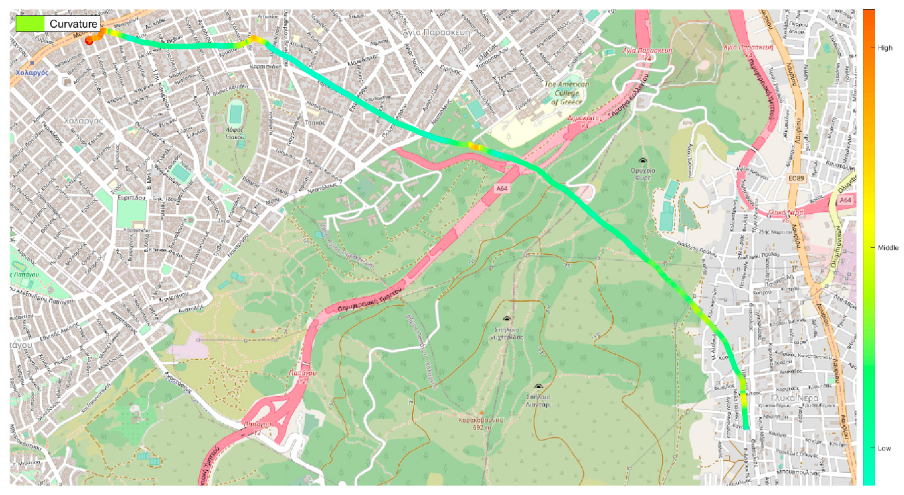
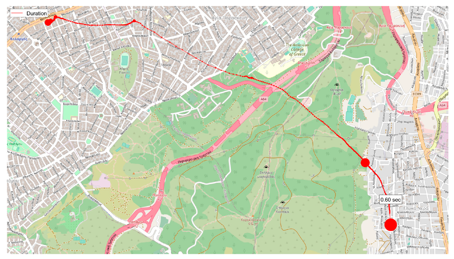
Function name
show_visualizations
Description
Exports 2D plots of the mouse movement trajectory, the deviations of both horizontal and vertical mouse coordinates over time, the curvature values across the trajectory and the duration of each coordinate point.
Syntax
function show_visualizations(A,InpImage,StimulusFigName,XYCoordsFigName,CurvatureFigName,DurationFigName,SaveToImage,SaveToFigure)
Input parameters
A: An array containing the tracked mouse movements of a trajectory. It can be given by functions movement_track or movement_track_seq.
InpImage: The visual stimulus image filename (e.g., “map.jpg”). All the main image file formats are supported.
StimulusFigName: Filename used to save the mouse movement trajectories as .fig and .png files.
XYCoordsFigName: Filename used to save the horizontal and vertical mouse coordinates over time as .fig and .png files.
CurvatureFigName: Filename used to save the horizontal and vertical mouse coordinates over time as .fig and .png files.
DurationFigName: Filename used to save the spatiotemporal distribution of the collected data as .fig and .png files.
SaveToImage: Flag indicating whether the figure(s) will be saved as .png image file(s) or not.
SaveToImage: Flag indicating whether the figure(s) will be saved as .fig MATLAB file(s) or not.
Output parameters
None.
Comments
The figures are created if a valid filename is provided. In order to omit a particular figure use symbols [] instead of a filename.
Example
show_visualizations(A,‘map.jpg’,‘StimFig’,[],‘CurvFig’,‘DurFig’,1,0);
In this example, the tracked mouse movements variable A is used, that corresponds to image “map.jpg”. Three figures are created as follows:
-
A stimulus figure named “StimFig” that depicts on the stimulis image the mouse trace (as a blue line) as well as the unique captured mouse points (as red circles)
-
A curvature figure named “CurvFig” that demonstrates the curvature at all the captured mouse points. By convention, low curvature values are depicted in green color while higher values are shown in red color.
-
A duration figure named “DurFig” that visualizes the duration time at each mouse point. Durations are depicted as circles where larger circle radii correspond to higher durations and vice versa.
The coordinates figure is omitted in this example, due to the empty filename parameter []. Finally, the figures are saved as .png files but not as .fig MATLAB files.
Function name
show_heatmap
Description
Create heatmap images of the mouse movement trajectory.
Syntax
function Heatmap = show_heatmap(A,InpImage,GaussStdDev,GaussScale,HeatmapFilename, HeatmapFigName,HeatIsolinesFigName,SaveToImage,SaveToFigure)
Input parameters
A: An array containing the tracked mouse movements of a trajectory. It can be given by functions movement_track or movement_track_seq.
InpImage: The visual stimulus image filename (e.g., “map.jpg”). All the main image file formats are supported.
GaussStdDev: Standard deviation of Gaussian filter.
GaussScale: Integer multiplication factor applied to GaussStdDev parameter that defines the kernel size.
HeatmapFilename: Filename used to save the source heatmap values as an image.
HeatmapFigName: Filename used to save the heatmap superimposed on the original image as .fig and .png files.
HeatIsolinesFigName: Filename used to save the 2.5D isolines surface of the mouse points’ spatial distribution as .fig and .png files.
SaveToImage: Flag indicating whether the figure(s) will be saved as .png image file(s) or not.
SaveToImage: Flag indicating whether the figure(s) will be saved as .fig MATLAB file(s) or not.
Output parameters
Heatmap: A 2D array containing the heatmap values.
Comments
The figures are created if a valid filename is provided. In order to omit a particular figure use symbols [] instead of a filename.
Example
HeatMap = show_heatmap(A,‘map.jpg’,32,6,‘heatmap.png’,”Heatmap2D’,‘HeatIsolines’,1,1);
In this example, the tracked mouse movements variable A is used, that corresponds to image map.jpg. The standard deviation of the Gaussian filter is set to 32 while a multiplication factor of 6 is used for the calculation of the kernel size. The function returns an array HeatMap that contains the calculated heatmap values. The heatmap is also saved as heatmap.png image file. A figure named Heatmap2D is created that depicts the heatmap superimposed on the original image. Additionally, another figure is created, titled HeatIsolines, that shows the spatial distribution of raw data using isolines. Finally, the figures are saved as .png files and as .fig MATLAB files.
Publisher’s Note: MDPI stays neutral with regard to jurisdictional claims in published maps and institutional affiliations.

