Article

Prostitution Arrest Spatial Forecasting in an Era of Increasing Decriminalization

by
Edward Helderop
1,*,
Tony H. Grubesic
1,
Dominique Roe-Sepowitz
2 and
Jorge A. Sefair
3
1
School of Public Policy, University of California Riverside, California, CA 92521, USA
2
School of Social Work, Arizona State University, Phoenix, AZ 85004, USA
3
Department of Industrial and Systems Engineering, University of Florida, Gainesville, FL 32603, USA
*
Author to whom correspondence should be addressed.
Urban Sci. 2023, 7(1), 2; https://doi.org/10.3390/urbansci7010002
Submission received: 11 November 2022 / Revised: 14 December 2022 / Accepted: 21 December 2022 / Published: 24 December 2022

Abstract

:
There is ongoing debate regarding the merits of decriminalization or outright legalization of commercial sex work in the United States. A few municipalities have officially legalized both the selling and purchasing of sex, while others unofficially criminalize purchasing sex but have decriminalized its sale. In addition, there are many other locales with no official guidance on the subject but have unofficially decriminalized sex work by designating specific areas in an urban landscape safe from law enforcement for commercial sex, by quietly ceasing to arrest sex sellers, or by declining to prosecute anyone selling or attempting to sell sex. Despite these efforts, it remains crucial to understand where in an urban area commercial sex exchanges occur—legalization and decriminalization may result in fewer arrests but is likely to increase the overall size of the sex market. This growth could result in an increase in sex trafficking victimization, which makes up the majority of commercial sex sellers in any domestic market. Given the distribution of prostitution activities in most communities, it is possible to use high-fidelity predictive models to identify intervention opportunities related to sex trafficking victimization. In this research, we construct several machine learning models and inform them with a range of known criminogenic factors to predict locations hosting high levels of prostitution. We demonstrate these methods in the city of Chicago, Illinois. The results of this exploratory analysis identified a range of explanatory factors driving prostitution activity throughout Chicago, and the best-performing model correctly predicted prostitution frequency with 94% accuracy. We conclude by exploring specific areas of under- and over-prediction throughout Chicago and discuss the implications of these results for allocating social support efforts.

1. Introduction

Crime prevention has long been a significant concern in many municipalities in the United States. As part of this effort, police departments, policymakers, and researchers have prioritized accurate crime prediction across space and time. These efforts have resulted in the rise of predictive policing [1,2]. The goal of predictive policing is to more efficiently direct limited police resources by predicting where and when crimes are likely to occur and who is likely to be responsible for those crimes. One can view virtually any quantitative analysis that results in a forecast of criminal activity and subsequent allocation of law enforcement resources as predictive policing. Integrating spatial and temporal elements into these models is essential because crime rates vary dramatically across the urban landscape, between neighborhoods [3], and even across streets [4,5].
Crime hotspot modeling has been a popular approach for visualizing and predicting criminal activity for several decades [6]. However, recent advances in modeling theory and computing power allow researchers to add complexity and fidelity to these models [7,8]. While more traditional, non-parametric approaches remain popular, including kernel density estimates [9], alternative analytical techniques show promise, including sentiment analysis [10], machine learning [11], and agent-based simulation [12,13] among others. Understandably, law enforcement agencies direct significant resources to develop accurate predictions of crime, hoping to reduce (or eliminate) interpersonal violence (e.g., assault, murder, rape), as well as property crimes throughout their jurisdictions [14].
The criminogenic factors that strongly correlate with one specific crime or type of crime (for example, property crime in general or muggings in particular) are different from those associated with other crimes or crime types. As a result, the best-performing crime prediction models aim to predict a single crime event or several closely-related crimes. In addition to the efficient application of law enforcement resources, there are several compelling reasons why predicting specific crime types is essential to quickly and efficiently provide services to victims. For prostitution specifically, this is a common motivation. Although many urban areas still criminalize the sale of sex with law enforcement arresting sex sellers, other locales are in the process of officially or unofficially decriminalizing sex work. This process means that the sex sellers are no longer criminals, but law enforcement may continue to arrest the customers (the people purchasing sex). A concurrent motivation for understanding where and when commercial sex transactions occur is providing social support services for sex sellers. Many sex sellers are victims of human trafficking (even in jurisdictions where sex work remains a crime), and many social service groups partner with law enforcement or operate independently to provide aid to these sex sellers [15].
At this point, it is essential to note that the treatment and portrayal of sex sellers in both media publications and research papers can be varied and often insensitive. In addition, there is an ongoing and unsettled debate over the potential benefits and drawbacks of decriminalizing sex work (more detail on this below) and even on the appropriate terms to respectfully describe the individuals engaged in these activities. Throughout the remainder of this paper, we will use the term ‘prostitution’ to refer to the specific crime of selling or attempting to sell sex. However, we will refer to the individuals engaged in sex work as prostituted persons or sex sellers rather than prostitutes. We do this primarily because the term prostitute has significant negative connotations associated with the crime and the broader morality surrounding commercial sex. Additionally, we will use the term sex trafficker to describe the third-party person who induces a person to participate in prostitution and the term customer to refer to the purchasers of commercial sex.
There are many compelling reasons for communities and social outreach groups to focus on commercial sex, including public health concerns [16]. In addition, from an economic perspective, there are important reasons to encourage sex sellers to find alternative income sources. These interventions may include efforts to assist individuals in avoiding sexually transmitted infections [17], assisting with basic needs like food or housing, or attempts to help individuals transition out of prostitution [18]. These voluntary interventions are also critically important in creating exit pathways for victims of sex trafficking.
The exposure of sex sellers to substantial physical and psychological abuse makes an escape without any outside intervention almost impossible—even in cases where a victim is not held physically captive. A repeated cycle of abuse, coercive control, and positive reinforcement by the trafficker can create a trauma bond, in which a sex seller may not realize they are a victim, and they rely entirely on the trafficker for food, money, and shelter [19]. In addition, sex sellers who are also victims of human trafficking may feel hopeless and isolated because of their movement to a new location where they know no one besides their trafficker [20]. This retention technique is a common tactic used by traffickers. Outreach agencies work to overcome these obstacles by acting as a supportive party to victims. Organizations provide various services, such as housing, healthcare, counseling, legal advocacy, employment opportunities, and escape from the situation [21].
Given this background, law enforcement and social service agencies will benefit from accurately identifying locations in an urban landscape home to high levels of commercial sex to best target where to provide services. This study aims to develop several spatially explicit and predictive models using a large set of urban variables operating across multiple spatial scales that help identify areas of prostitution in the urban landscape and deliver vital social services to the community. We demonstrate the efficacy of these models in the city of Chicago, Illinois, but the results are generalizable to any urban area in the United States.

2. Background

2.1. Spatial Crime Forecasting

Before developing more sophisticated statistical techniques that quantified the relationship between facets of crime and demographic or areal characteristics, scholars typically explored the relationship between crime and space via mapping (as early as the mid-1800s) [22]. These early efforts mapped the locations of crimes and one or two other demographic factors in an area. As the field of spatial statistics matured, it became possible to explore how the characteristics of a specific place impacted the frequency, type, and likelihood of crimes, which allowed for initial work in crime forecasting [23]. Throughout the 1970s and 1980s, a variety of place-based crime theories were proposed, including the routine activity theory [24], environmental criminology [25], and the scanning, analysis, response, and assessment process [26], among others. Their common element is recognizing that the location of the crime is important [27,28].
As spatial statistical understanding and available computing power increased over the past several decades, so did the overall sophistication of crime forecasting techniques. At their most basic level, forecasting methods employ simple statistical regressions with a relatively coarse resolution [29], while more complicated efforts increase the spatial (or temporal) resolution and employ sophisticated machine learning techniques [30]. For example, in 1982, Brown [31] used a basic spatial regression to identify significant clusters of violent crime throughout Chicago. Similar efforts matured over the next several decades, with modern studies employing neural networks to process enormous amounts of data and forecast crime over large areas with fine spatial and temporal resolutions [32].
Crime forecasting remains challenging, with explanatory criminogenic factors varying between crime types, urban areas, and even the scale at which one examines the crimes. Ansari, Hofkens, and Pianta (2020) [33] find that early childhood school absenteeism is strongly related to the likelihood that a teenager or young adult will end up arrested for a crime. This outcome mirrors other work that finds links between the likelihood of an arrest and a general index of the socioeconomic status of an arrested individual [34]. In addition to the relationship between individual characteristics and crime, many studies examine how the environmental characteristics of an area make it likelier to play host to crimes. Public disinvestment in an area is correlated with increasing crime rates, as is the presence of crime itself. There is evidence of a vicious cycle in which visible crime in an area makes future crime in that same area likelier [35].
However, not all relationships between crime and its determinants are as intuitive or straightforward. For example, MacDonald, Hipp, and Gil (2013) [36] found that neighborhoods throughout Los Angeles with higher immigrant densities have lower crime rates. However, Kubrin and Ishizawa (2012) [37] found the opposite—areas with higher immigrant densities had higher crime rates than expected. A close examination of these and similar studies reveal the importance of forecasting specific crime types and differences between urban areas. The results also underscore the importance of specifying the scale at which a study operates. Property and violent crime, for example, occur in different locations, and one can categorize each category of crime by unique sets of urban features [8,38].

Potential for Bias in Predictive Policing

Predictive policing is a data-driven strategy that uses large datasets dealing with historical crime patterns to predict future elements of crime, including crime locations, perpetrator characteristics, and victim characteristics. There is debate over whether this type of data-driven predictive policing is biased. This debate occurs in traditional media [39,40,41] and in academic literature [42,43]. There are concerns that predictive policing will entrench historic racial or socioeconomic biases held by the police and engrained within the data sources. Specifically, by training on historical data, which may be biased, the resulting predictions may also be biased. For example, in the United States, a Black person is five times likelier to be stopped by the police without cause. Furthermore, a Black person is twice as likely to be arrested as a white person [39]. However, recent empirical work found no evidence of systemic bias after the Los Angeles police department deployed predictive policing algorithms to determine where future crimes were likeliest to occur [42].
Nevertheless, it is essential to acknowledge that the merits of predictive policing remain an open question within the literature—even as the underlying algorithms evolve and improve. For this paper, we use historic arrest data in the city of Chicago. Within this context, it is critical to acknowledge that every crime incident within a city (e.g., Chicago) does not yield an arrest. This disconnect happens for many reasons, including racial and economic bias on behalf of law enforcement agencies [44], police presence bias, in which most police presence concentrates in relatively few neighborhoods [45], and the willingness of specific neighborhoods to call the police or tolerate crime [46]. As a result, our training dataset captures only arrests—it does not capture all crimes that occur in a city.

2.2. Commercial Sex in Urban Areas

Modern studies that focus primarily on predicting the location of prostitution in an urban area are rare [47]. Unsurprisingly, there is more focus on crimes that attract more public attention via their immediate visibility in a community—gun crimes, for example. Additionally, some cities in the United States have begun officially or unofficially decriminalizing the sale of sex (this may take the form of continuing to arrest and prosecute the purchasers of sex in an attempt to shrink the overall size of the sex market; [48]). This strategy reflects a growing consensus that the sex sellers themselves are primarily victims and arresting them for the sale of sex is counterproductive when it comes to the larger goal of helping people leave commercial sex work [49]. Although arrests for prostitution in an area may decrease after decriminalization, the actual size of an urban area’s sex market can increase, and the redirected police resources and attention can contribute to or be perceived as more permissive of additional sex trafficking [50]. As a result, accurately identifying urban characteristics that lead to high amounts of prostitution activity is a crucial way to combat sex trafficking, even in an environment in which the sale of sex itself is not a criminal activity [51]. It is challenging to derive any detailed information when examining arrests of human trafficking, specifically. While obviously a crime, it is rare for suspects to be arrested for trafficking rather than an attendant crime that is often performed simultaneously. Furthermore, when arrests do occur, they rarely occur at the ’scene of the crime,’ so to speak, but rather often at a trafficker’s place of residence or at a controlled location arranged via a law enforcement operation. As a result, the spatial data contained within the arrest record will not necessarily shed any light on where future traffickers whose existences are unknown could be interdicted.
Until 2013, prostitution was a felony offense in the state of Illinois. Since then, it was recategorized as a misdemeanor, although one that can still carry jail time. This shift reflected a belief among judges and district attorneys’ offices throughout the state that prosecuting sex sellers is ineffective in rehabilitating them and combating exploitative sex work and sex trafficking. In turn, the implemented changes influenced police behavior, dramatically reducing the number of prostitution arrests made each year in Chicago. In 2021, for example, there were only 21 prostitution arrests, down from around 6000–7000 per year during the aughts.
Nevertheless, official or unofficial decriminalization of sex work in the United States is rare enough that we must continue to explore its impacts on the sex market size, the sex sellers themselves, and host communities. Cunningham and Shah (2018) [52], for example, found that the decriminalization of indoor sex work in a Rhode Island community did increase the overall size of the market (specifically, there were more participants and more exchanges) but resulted in fewer reported rape offenses and fewer reported sexually transmitted infections by the sex sellers. Raphael (2018) [53], however, found that decriminalization leads to more sex trafficking, primarily because the traffickers see decriminalized sex markets as safer and more lucrative. In fact, the frequency of sex sellers that are also or were also victims of human trafficking is high; with some research finding that prostitution is the primary or only motive behind most trafficking cases in the United States [54,55,56]. Although a full exploration of the current debate about the benefits and drawbacks of sex work legalization is outside the scope of this manuscript, it is essential to note that it is not a settled topic [57].

3. Methods

3.1. Study Area and Data

This study takes place in the city of Chicago, Illinois. Chicago is the third-largest city in the United States by population and is located along the southwestern shore of Lake Michigan. It is a diverse, densely-settled region, home to around 2.7 million people. Chicago provides an ideal location for our study for several reasons. First, the city’s stance on the criminality of prostitution also mirrors most other cities, with a recent goal of reducing arrests for nonviolent crimes [58], even if the sale of sex remains technically illegal. Second, Chicago is committed to generating and maintaining robust, publicly available data on various municipal topics. Detailed spatial crime data, in particular, can be challenging to find in many U.S. cities, and its existence in Chicago means it is possible to generate a spatially explicit, high-fidelity crime prediction models for the city. Third, Chicago publicly provides essential infrastructure data (e.g., walking paths, hospitals, bus stops). When combined with relevant social and demographic data, this mix of indicators provides a strong foundation for empirical modeling. Lastly, Chicago’s geographic and demographic profile is similar to many other large cities in the United States, so our results are broadly generalizable to other locations.

3.2. Forecasting Prostitution

The primary goal of this paper is to develop prostitution forecasting models rather than explanatory models for prostitution. Methodologically, this distinction is important because the development of predictive models diverges from explanatory models in several ways [59]. Most analysts evaluate the quality of explanatory models using goodness of fit and statistical significance metrics. Furthermore, efforts to avoid misspecification, Type I and II errors, multicollinearity, endogeneity, heteroscedasticity, and autocorrelation are essential for developing viable explanatory models. However, this is not necessarily the case for predictive models. In contrast, key metrics for evaluating predictive models include parsimony, predictive accuracy, and practical deployment [59]. As a result, obedience to strict statistical principles in developing prostitution forecasting models is not as essential as it might be if our goal was to develop an explanatory model. We recognize these differences and use a suite of variables that provide the most practical, parsimonious, and predictive forecasts of prostitution activity in Chicago. Additionally, while we highlight some metrics for evaluating explanatory models (e.g., model fit, statistical significance), this is for the convenience of readers and is not necessarily central to evaluating model performance.

3.3. A Model for Predicting Locations of Prostitution Activity

We use a wide variety of data sets for the modeling efforts in this paper. Although spatial crime modeling work is relatively common, prostitution-specific work is limited. As a result, this demands that we cast a wide net for potential urban criminogenic factors. Using several combinations of these factors, we performed a type of ablation study in which neural network models were trained using different sets of input variables in order to determine the set of independent variables that results in the ‘best’ model (the one that achieved the highest predictive accuracy). Specifically, we generated, trained, and tested models using a wide variety of the different combinations of input variables to determine which unique set resulted in the ‘best’ model, judging by predictive accuracy. By and large, these variables capture measures of urban land-use, social disorganization, public (dis)investment, and criminal opportunity. While criminogenic factors for different crimes are often similar, the construction of high-fidelity models requires identifying those unique to the specific crime in question. For a complete list of datasets used to build our models and their provenance, see Table 1. All of these datasets come from the Chicago Data Portal [60], the most recent five-year American Community Survey (ACS) survey (2015–2019) [61], or the North American Industry Classification System (using Esri Business Analyst; [62]). In addition, we use four basic shapefiles to delineate our study; a Chicago city boundary shapefile [60], a Census block group shapefile [63], a Cook County address point shapefile [64], and a Chicago Police Department beat shapefile [60].

3.3.1. Geocoding Masked Crime Data

The crime data provided by the city of Chicago is, understandably, masked. Many municipalities mask crime data to preserve household-level anonymity. Specifically, each crime is associated with an address in the city of Chicago, and the street number of each address is anonymized as follows: ‘2500 Main St.’ becomes ‘25XX Main St.’ The last two digits of each street number are replaced by ‘XX’, regardless of the number of total digits in that street number. The street name is not changed, nor is the police beat in which the crime occurred. Geocoding masked data is challenging. It requires minimizing potential errors while maintaining sufficient anonymity in any publications to satisfy the original mandate of the dataset. In order to achieve this, we followed the medoid geocoding technique [65].
For its application in Chicago, the medoid technique requires the complete address point database available via the Cook County Assessor’s office. For each crime observation, we consider all of the possible matching addresses. For example, if a crime observation reads ‘25XX Main St.,’ all valid addresses that fall along the 2500 block of Main St. are grouped into a working list. This list would include 2500 Main St., 2510 Main St., 2512 Main St., and any additional addresses that conform. This working list represents all potential addresses for a given crime—known as candidate addresses. Next, we remove each candidate address that falls outside the police beat associated with the crime observation. This step removes those addresses from the wrong street for situations where two streets have the same name. If the candidate list contains only two possible matches, we randomly select one and use that address as the ‘correct’ address for the crime event. Finally, we generate a convex hull around the potential address set for crime events with more than two potential addresses and select/assign the medoid for geocoding. Specifically, the medoid address is the centermost address—the address that minimizes the aggregated distance to each other address on the list. See [65] for more technical details.
It is worth noting that while this process seeks to minimize the geocoding error, there is no guarantee that it identifies the correct address from the masked observations. Instead, our efforts for geocoding crime events to the centermost candidate address help reduce the likelihood of large spatial errors in the geocoding process. This reduction in spatial error is critical for subsequent steps in the analysis process, including aggregating crime event data into Census administrative units or some other type of spatial tessellation (details to follow). Based on the average size of the convex hulls and a manual spot check performed on a random subset of the prostitution data, we are confident that all or nearly all crimes were associated with the correct polygon/administrative unit during the aggregation process.

3.3.2. Hexagonal Fishnet Aggregation

We chose to use hexagonal cells as the unit of analysis for these models. There are three primary benefits to using hexagons. First, the centroid-to-centroid distances of hexagonal tessellations are constant, unlike square grids (which, when using a queen’s contiguity rule, have two different centroid-to-centroid distances—one for the neighbors that share an edge and one for the neighbors that share only a corner). This feature is critical for many fundamental spatial measurements used for the modeling process. Second, hexagons reduce potential sampling bias for prostitution events because the edge length to cell area ratio is smaller for hexagonal tessellations than for traditional square grids. Third, any crime event/point within a hexagon is closer to the hexagon centroid than any given point in an equal-area square. Again, these geometric features are critical for many fundamental spatial analysis routines.
Nevertheless, one fundamental limitation to using hexagonal grids is less of an issue for modern spatial analytics than those used years ago. Namely, hexagonal tessellations were more computationally difficult to generate and store. Hexagons also required more computational effort for developing spatial weights. Today, these historical challenges are largely moot and do not impact our geocomputational efforts. We conducted a sensitivity analysis to determine the ideal hexagonal cell size, which was 0.2 square kilometers. In order to arrive at this cell size, we fitted different models at a variety of different cell sizes, ranging from 0.05 square kilometers to 0.5 square kilometers. It is challenging to identify the ‘best’ cell size for studies like this—which is one reason that many rely on simply aggregating to Census block groups or tracts. Ultimately, we feel justified in our use of 0.2 square kilometer cells for several reasons. First, and perhaps most importantly, the same models trained at different cell sizes all had relatively similar results. While the fidelity varied (and was maximized at 0.2 square kilometers), the general patterns revealed by the models were consistent across the different sizes, providing some confidence that our results at a given size were not anomalous. Second, a hexagonal cell of 0.2 square kilometers captures an area of the urban landscape at which many of the criminogenic factors that we use to inform our model are operating. Third, by also including our explanatory factors as second-order effects (more detail on this below), the overall size of the cell matters slightly less—further mitigating the potential negative effects of choosing the ’wrong’ size.
The aggregation process for our various datasets included three steps. First, we assigned point data to their intersecting hexagon cells as a count (e.g., the total number of prostitution arrests in each cell was summed and assigned to that cell as an attribute). Second, since the ACS data is available only at the block group level, we use a weighted average approach to assign attributes to each overlapping hexagon. Specifically, each hexagonal cell adopted the weighted value of the data from any intersecting block group(s) based on the total areal coverage of that block group found in a given hexagon. For example, a hexagonal cell that contained 80% of one block group and 40% of another would be assigned a total population equivalent to 80% of that first block group plus 40% of the second. We acknowledge that this process introduces errors. However, because many block groups in Chicago are similar in size and density, this error does not dramatically impact the models. Nevertheless, a higher resolution source of these data (e.g., by the block rather than block group level) would further increase the fidelity of our models. Finally, each dataset was also spatially lagged across our study area. We assign the average second-order neighbor value (comprised of the six neighboring hexagons) to the hexagonal cells for each variable.
It is also worth noting that instead of introducing a custom tessellation, we could aggregate all of our point data to the block groups themselves. This alternative spatial conceptualization of the data would remove any error introduced by the polygon-to-polygon aggregation. In attempting this, however, we found that the irregular shapes of the block groups themselves introduced significantly more error via the presence of odd edge effects. Furthermore, it was more challenging to account for the second-order neighbor effects of several variables of interest. As a result, we found that the models using homogeneous hexagonal cells were higher fidelity than those using block groups as the spatial unit of analysis.

3.4. Model Generation

From a modeling perspective, there are many different options for developing a predictive framework, including classic inferential approaches [66] and more novel machine-learning techniques [67]. This paper explores both—evaluating the predictive performance of a spatially lagged logit regression model and an artificial neural network (ANN) model. We inform our model using a combination of criminological theory (detailed previously) and an exploratory data analysis to determine the ‘best’ suite of predictive variables. Specifically, by training multiple models with a range of available variables for Chicago, we identify the varying spatial scales of the predictive factors. For example, while bus stops exhibit a strong relationship to crime, the effects are typically hyperlocal—occurring close to the stops. In contrast, our exploratory analysis reveals that hospitals exhibit a weak anti-criminogenic over a larger area, so their presence as second-order factors improved our ability to predict prostitution.
Chicago and the state of Illinois have recently begun taking steps to decriminalize prostitution unofficially [68], and as a result, the prostitution arrest data for the city became less reliable beginning in 2017. We used prostitution arrest data from 2009 to 2016, inclusive for the model training and the primary testing dataset. While we have data from earlier years (since 2001), the city’s character has changed fairly significantly over the past several decades, and our infrastructure and demographic data are increasingly uncertain when considering historical arrests. After 2016, the number of prostitution arrests began dropping (e.g., there were only 21 prostitution arrests in 2021), so including these data may have produced a less reliable model. For this reason, this type of model would be even more effective in cities that were not decriminalizing prostitution—more recent arrest data results in a higher-fidelity model.
It is also important to note that prostitution arrests in Chicago concentrate in a handful of locales—a common phenomenon for urban sex work in the United States. As a result, the prostitution arrest counts for our cells exhibit a long-tailed distribution, with the majority having no prostitution arrests during our analysis period. For example, one cell had nearly 3000 arrests (averaging almost 1.5 arrests per day for the entire six-year period). Additionally, not all crimes result in an arrest, with the relationship between the two varying between neighborhoods and over time. Finally, the broader applications of studies like ours are to help law enforcement agencies and social outreach groups utilize their resources more efficiently. For these reasons, we sought to identify areas in the city associated with high prostitution rather than predict the specific count of arrests in each cell. As a result, we used a threshold value for the arrest counts to generate a binary high/low prostitution value. Based on a review of the frequency distribution of prostitution arrests in our study area’s cells, we chose a threshold value of three arrests. Any cells with more than three arrests were designated high-prostitution cells, while those with three or fewer arrests were low-prostitution. Interestingly, as the threshold value increases, our models’ efficiencies increase, indicating that our suite of independent variables effectively identifies areas of increasingly higher prostitution. Given the consistent performance of our models across a wide set of possible threshold values, we are confident that our results are not an artifact of the specific threshold value for which we report results for the remainder of this paper.
We used an 80/20 training-testing split for each of the models. Specifically, we randomly chose 80% of our cells for training the models and used the remaining 20% to test predictive performance. We used a grid search to identify the optimal values for the neural network size (e.g., number of hidden layer units; 45) and decay (e.g., regularization parameter; 0.05). Next, we generated a confusion matrix for each model to indicate the number of correct positive and negative predictions and the number of incorrect positive and negative predictions. We evaluated the model efficiency from that matrix by summing the correct predictions (positive and negative) and dividing by the total number of observations. These model efficiencies were the metrics by which we determined the appropriate suite of independent variables. In the next section, we discuss the results from our ‘best’ models—those that exhibited the highest efficiencies and were thus the most effective at accurately predicting high- and low-prostitution cells. In addition, we explored our model residuals to look for systematic incorrect predictions and manually identify any missing predictive factors. All model training and analysis was performed in R, using the packages ‘MASS’ and ‘nnet’.

4. Results

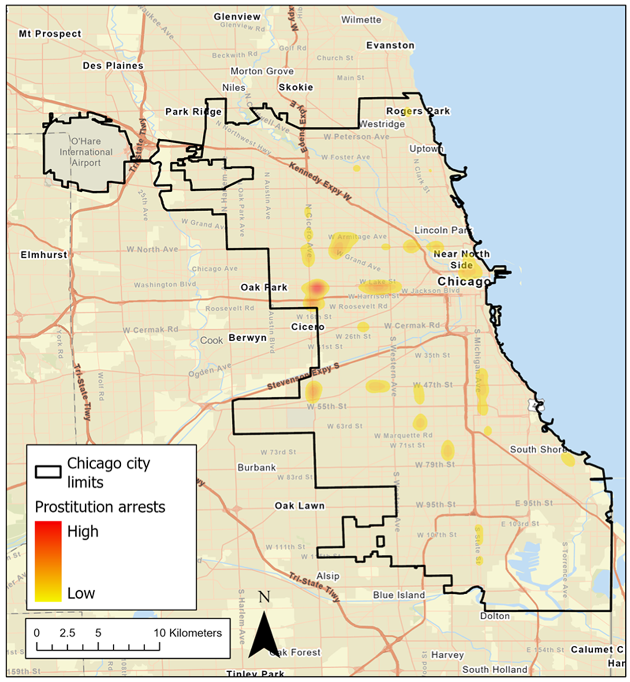
4.1. Spatial Footprint of Prostitution Arrests in Chicago

Prostitution arrests in Chicago are highly spatially concentrated (Figure 1). The primary epicenter of prostitution is at the intersection of three neighborhoods: the northwest corner of Lawndale, the southwest corner of West Garfield Park, and the southeast corner of South Austin, on the city’s west side. This cluster of activity centers is at the intersection of Illinois Route 50 (running north–south) and Interstate 290 (running east–west). From here, prostitution arrests remain relatively high on the corridor to the east, parallel to 290, especially on the north side of the highway. Interestingly, there is a duplicate pattern to the north, with an east–west corridor of prostitution running next to Route 64, terminating in another hotspot in the Near North and Gold Coast neighborhoods. Finally, the city’s south side also sees scattered areas of high prostitution, notably including a cluster in Washington Park, running parallel to Interstate 90.
Many of these neighborhoods experienced a significant decline after the 1960s, a result of a combination of riots after the assassination of Martin Luther King Jr., the closure of major industries (such as Sears and Western Electric), and the departure of many residents who could afford to leave (Steans Family Foundation, 2009) [69]. In a book about urban inequality, Kozol (2012) [70] noted that Lawndale had one supermarket, one bank, and 99 bars. However, this is not the case for every neighborhood that experiences increased prostitution arrests. For example, the area around the downtown loop is expensive and hosts high-end commercial and retail spaces. Prostitution arrests may be concentrated here due to higher-end clientele and additional police presence.

4.2. Model Performance
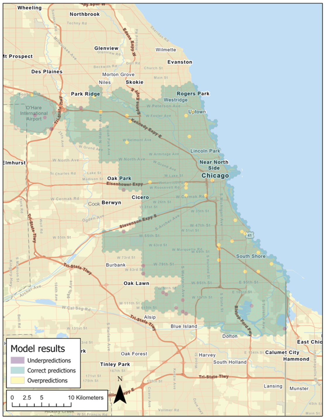
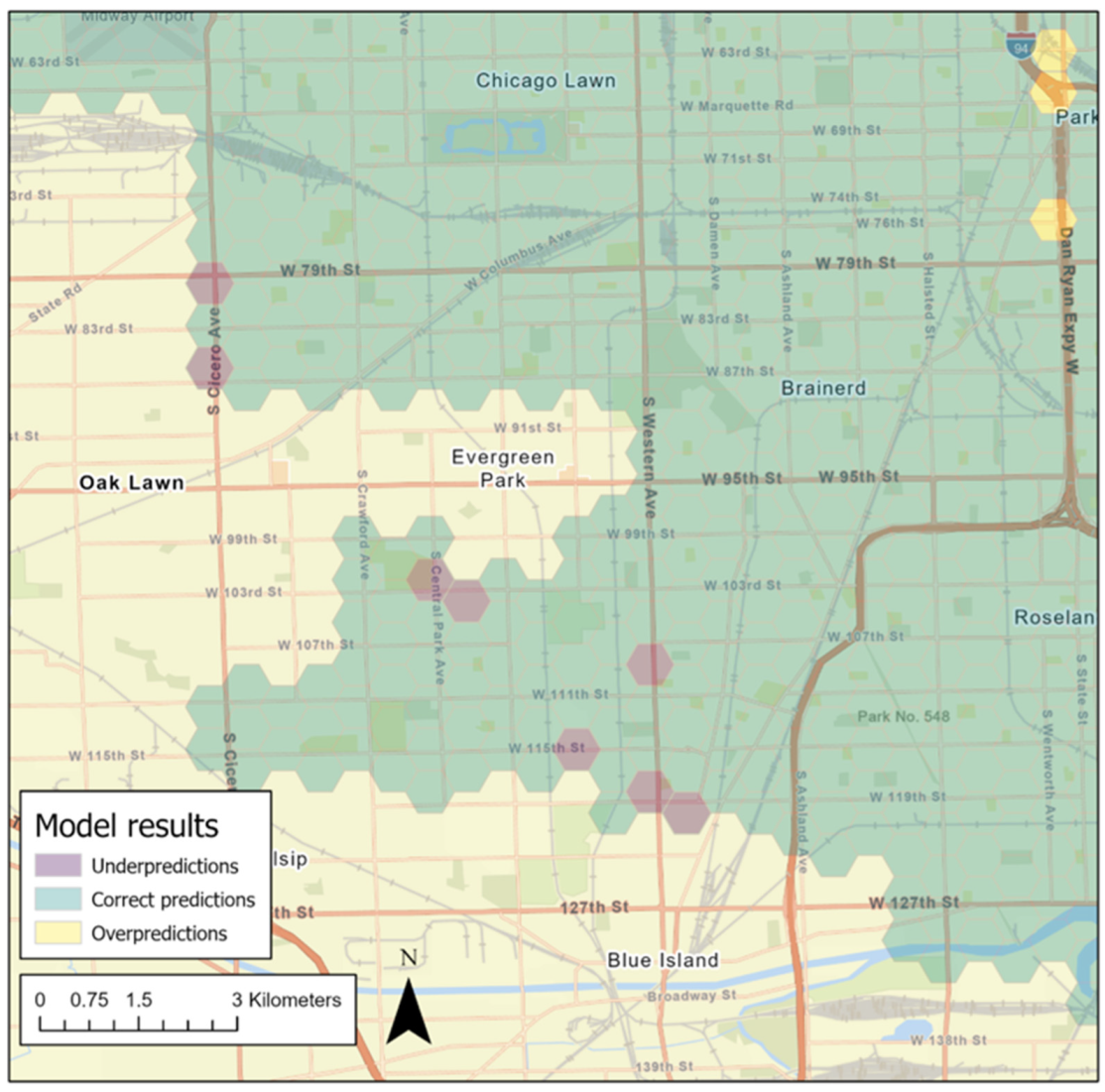
Both the logit model and neural network performed satisfactorily in terms of prediction power. However, the neural network outperformed the logistic regression in its predictive efficiency. The logistic regression had an 81% efficiency on the test set—in other words, it correctly classified 81% of the cells as either high or low prostitution, while the neural network had an efficiency of 94%. Of the 81% of the cells that the logistic regression correctly predicted, the neural network correctly predicted 99% (in other words, 80% of the cells in the study area were correctly predicted by both models). Of the rare cells that the logistic regression correctly predicted but the neural network incorrectly predicted, approximately two-thirds were low-prostitution cells (that the neural network incorrectly predicted as high-prostitution), with the remaining one third the opposite. Nevertheless, there were significantly more cells that the logistic regression predicted incorrectly that the neural network predicted correctly. Of these cells, approximately 80% were low-prostitution cells that were overpredicted by the logistic regression.
The neural network does not provide any interpretable information about the individual impact of each independent variable on the model. Although there are weights associated with the input layer of our neural network, without specifically training the model to provide interpretable parameters, the weights themselves do not shed light on the importance of individual input variables. However, that is not the case for the logit regression, which produces easily interpretable variable coefficients. These coefficients are not the same as neural network weights, and there is no guarantee that the variables that are identified as important by the logit regression are important in the ANN. Nevertheless, examining the logit regression coefficients does provide some information on the relationships between prostitution arrest frequency and the input variables. Table 2 contains the coefficient estimates and p-values for each of the variables in the model. For example, high prostitution cells are closer to major roads, are areas with low socioeconomic status, contain more liquor stores, bars, strip clubs, bus stops, more problem landlords, and have a higher black population. Hospitals provide a protective effect, with a significant negative correlation with prostitution for cells containing part of a hospital. That protection may extend to neighboring cells to some degree, but that relationship is not significant. Police station presence is not significant, nor are schools or parks. These results are in line with similar (previous) studies. Many of these factors are consistently criminogenic in urban areas in the United States. Several of these variables exhibit moderate multicollinearity, which is not a factor of concern for prediction [59,71]. Additionally, the neural network residuals exhibit significant spatial autocorrelation, with a global Moran’s i value of 0.23, and an associated p-value of <0.001. However, because we are interested in the predictive accuracy of our models, rather than drawing conclusions about the explanatory impact of different input variables (as would be the case in an explanatory model), no explicit corrections for spatial autocorrelation are needed or employed. Furthermore, due to the fact that neural networks are modeling non-linear relationships between the various variables, they rarely benefit from spatial autocorrelation correction to begin with [72,73,74].

Model Residuals

Figure 2 is a residual map of the neural network results. This model correctly classifies 94% of the cells across the city of Chicago. By examining the model’s residuals, we can identify problematic areas that the model cannot predict correctly. Because prostitution cases are such a long-tailed phenomenon in Chicago, a null model predicting low prostitution in every cell across our study area would result in an efficiency of around 60%—simply because that number of hexagons have three or fewer (usually zero) prostitution arrests in our dataset. The residual errors exhibit a relatively even distribution across the study area. Of note is that when the prediction is incorrect, our model tends to overpredict (i.e., our model predicts high prostitution in an actual low prostitution cell). Furthermore, most overpredictions occur along major highways or freeways, particularly highway interchanges. These cells may exhibit many characteristics associated with prostitution but are areas where prostitution arrests may not be possible. For example, there may be no pedestrian paths adjacent to these highways, or arrests may happen in developed areas immediately adjacent to these cells. Although we hoped to correct this by including pedestrian paths as an independent variable, that correction is insufficient. This result may also arise because all crimes in our dataset are associated with an address—and arrests may occur in these cells but are connected with the address of a neighboring cell because highway interchanges have few, if any, actual address points located alongside them.
Model underpredictions are rare (under 1% of the cells in the study area were underpredictions). These are cells in which the neural network incorrectly predicts low prostitution arrests. There are too few of these to discern a consistent pattern, but most occur in southwestern Chicago (see Figure 3). These neighborhoods are a mixture of large manufacturing, freight, and transportation lots, alongside residential streets. The neighborhoods are not impoverished or home to many other crimes, as a rule. It is challenging to identify any patterns for such a small sample, however—additionally, judging by the cells’ locations along the edge of our study area, there may be an edge effect influencing our model’s ability to predict this areas for which we are not accounting. Alternatively, it is possible that these areas are coming up as false positives due to the preponderance of highway interchanges, train track infrastructure, and the relative proximity of the Chicago-Midway airport. Areas with concentrated travel and shipping industry are often home to a high concentration of cheap hotels and motels that may serve as locations where commercial sex markets operate [15].

5. Discussion

In testing many potentially criminogenic factors in many different configurations, we determined the ‘best’ suite of predictive variables for the location of high prostitution arrests in Chicago. Many of these are unsurprising—these variables were initially selected as potential inclusions based on previous literature that found them to be criminogenic in studies that were at least similar to ours. However, most crime forecasting studies primarily examine violent crime. Because we were interested in forecasting prostitution, we explored a broad set of potential criminogenic factors, anticipating some differences between the sale of sex and violent crimes. To begin with, and in line with previous studies that have examined prostitution, street proximity and density are strongly linked with increased prostitution presence [75]. Road infrastructure like this provides some access for street-based commercial sex sales. Additionally, long-haul truckers patronize commercial sex sellers at particularly high rates [76]. As a result, prostitution activity often concentrates along major shipping and logistics corridors [15].
The presence of problem landlords is also a strong predictor of prostitution activity. To some degree, this factor likely reflects the overall character of a neighborhood. Specifically, one often finds problem landlords in impoverished neighborhoods that receive less public investment. In U.S. cities, these areas often have a majority of Black residents [77]. This result is a complicated mélange of factors, but broadly speaking, these areas are home to more crime in general, including prostitution. Additionally, these neighborhoods may attract more police presence, thus potentially resulting in more arrests [78]. Liquor stores and bars are similarly generally criminogenic [79,80] and may also reflect the overall character of their neighborhoods [81]. Combined, many of these factors may create a neighborhood with low social capital or social cohesion, thus creating situations in which the residents of an area are accepting of or at least ambivalent towards sex work.
It is important to note that not all high-prostitution areas in Chicago fit this mold. There are prominent hotspots in and immediately adjacent to wealthier regions of the city, such as the neighborhoods north of the downtown loop. Recall that the dataset indicates the location where the arrest occurred—although many of the sex sellers may not live in this area, they may be conducting business there. For instance, wealthier clientele may live and work in or near this region of Chicago, and commercial sex sellers who target higher-end clients may ultimately meet those clients in hotels or bars in this area. Additionally, the area may attract additional police presence and attention, and residents and workers in the area may be more willing to call the police if they notice anything amiss.

5.1. The Future of Decriminalization

Predicting prostitution will become even more critical in a future where decriminalization is common. By identifying the locations where the commercial sex market operates, law enforcement agents can arrest the facilitators of the sale of sex, including the purchasers and traffickers. Meanwhile, social service groups can reach victims to provide various types of aid. These efforts include providing exit pathways for sex seller that are (or were) trafficked. Trafficking itself is a challenging crime to study. In Chicago, for example, across 21 years of crime data (2001 to 2021), there were only 77 trafficking arrests, averaging fewer than four per year. This outcome is in line with the national average, in which only a few hundred human trafficking arrests are made yearly in the U.S. To the degree that human trafficking victims are forced to engage in sex work, understanding the spatial footprint of the commercial sex market remains important, even in a world where the act of selling sex itself is decriminalized or legal. While much of the attention focuses on social media and online commercial sex work, the reality is that sex work still requires the commercial sex seller to meet with the buyer, which requires being seen, and in some cases, being arrested for unlawfully selling sex. This requirement also includes the trafficker and the sex trafficking victims primarily using hotels and motels to live [82]. As communities develop new interventions to address sex trafficking, including victim-less undercover work looking for traffickers, this location information helps law enforcement make data-driven policing decisions. This predictive location information can also assist with targeted human trafficking identification and response training for the area, including convenience stores, bars, hotels, motels, liquor stores, and strip clubs. Social services will be able to prioritize their limited resources to focus on specific areas for street outreach and, if possible, establish agency locations local to the high prostitution- high sex trafficking victimization areas.
Meanwhile, decriminalization continues apace for sex work. In Nevada, there are eight rural counties in which prostitution is explicitly legal. This legality is codified in law. In other jurisdictions, the officiality of decriminalization varies. In some counties, district attorney officers have explicitly said they would not prosecute sex sellers for selling sexual acts (e.g., Washtenaw County, Michigan). In others, there may be no public statement, but arrests are declining, and actual convictions of sex traffickers and sex sellers are becoming rarer. This strategy is controversial. The criminalization of commercial sex work may further victimize sex sellers, leading them to avoid seeking medical treatment or going to the police when they become victims of a crime or are in danger [83]. However, in more than 30 cities in the U.S., being arrested for prostitution (as an adult) results in a plea agreement to attend a diversion program focused on assisting the participants to exit prostitution and connecting them to treatment, counseling, and support services. These diversion programs allow the victim to have contact with those outside the commercial sex work domain (e.g., buyers, traffickers, and other sex sellers) and, in some cases, give them the tools to leave sex work altogether. There is also evidence that legal strip clubs and brothels attract potentially violent sex offenders—they patronize these industries instead of committing acts of violence against criminalized sex sellers [84]. However, decriminalization may also increase the overall size of the sex market, particularly if communities decriminalize both buying and selling sex.

5.2. Limitations and Future Work

From the standpoint of predicting prostitution on its own, we face one major limitation common to many criminology studies. Arrest data, including comprehensive datasets like Chicago’s, are somewhat biased by the behaviors, priorities, and policies of law enforcement agencies, among other parties. Not all crimes in a city result in an arrest. There are many reasons for this, including racial bias, district attorney priorities, the willingness of residents to call the police, and historical neighborhood bias, among others. In addition, the specific arrest data we used to train our models are several years old due to the unofficial decriminalization of the sale of sex in the city of Chicago and the attendant decrease in arrests. As the city’s urban landscape changes over time, the outdated prostitution arrest data will fare worse. Prostitution arrests are much lower than they were several years ago, although this does not reflect a decrease in the size of the overall sex market in Chicago. In the long-term, this means that the spatial prediction of the location of commercial sex markets in cities that have decriminalized the act of selling sex will become increasingly difficult. Eventually, as arrest data becomes too dated to train a high-fidelity model, an alternative data source will be needed.
Two projects are ongoing to expand this work. The first is a simple expansion of this methodology to other cities in the United States. This expansion aims to demonstrate the overall resilience of our model construction and, more broadly, to identify which urban characteristics associated with prostitution locations can be generalized between different cities. Ideally, this will result in a better understanding of the urban conditions that promote (and discourage) prostitution. The second is a qualitative expansion of this work in which we are interviewing specifically victims of human trafficking forced to engage in commercial sex exchanges to understand their movements in and between cities. From this, we hope to target the portion of sex work that is explicitly linked to human trafficking, and it may shed light on other urban features that our model should include to increase its fidelity further. An additional project that may provide significant benefits to quantitative criminology in general would be to more rigorously examine the differences between different predictive models. Although we utilized both a logistic regression and an ANN, we did not structure the study to comprehensively compare the two in their predictive power or structure. Shedding light on the types of relationships that different frameworks are best able to model could help increase predictive efficiency across the field more generally. It may be possible to examine the rare cells in which the logistic regression outperformed the neural network to determine why—depending on those findings, the neural network model could be improved.

5.3. Conclusions

In this paper, we built several models that predicted the locations of prostitution arrests throughout the city of Chicago. We used a comprehensive set of training variables, and our best model accurately identified high-prostitution areas over 94% of the time. This work has important implications for helping track, predict, and prevent human trafficking. It will enable law enforcement groups and humanitarian outreach agencies to better direct their limited resources to help sex sellers transition out of sex selling situations while continuing to target traffickers themselves.

Author Contributions

Conceptualization, E.H. and D.R.-S.; methodology, E.H. and J.A.S.; validation, E.H. and T.H.G.; formal analysis, E.H.; data curation, E.H.; writing—original draft preparation, E.H. and D.R.-S.; writing—review and editing, E.H., T.H.G. and J.A.S.; visualization, E.H.; supervision, T.H.G.; project administration, J.A.S.; funding acquisition, J.A.S. All authors have read and agreed to the published version of the manuscript.

Funding

This material is based upon work supported by the National Science Foundation under Grant No. 2039917.

Conflicts of Interest

The authors declare no conflict of interest and the funders had no role in the design of the study; in the collection, analyses, or interpretation of data; in the writing of the manuscript; or in the decision to publish the results.

References

  1. Perry, W.L. Predictive Policing: The Role of Crime Forecasting in Law Enforcement Operations; Rand Corporation: Santa Monica, CA, USA, 2013. [Google Scholar]
  2. Meijer, A.; Wessels, M. Predictive policing: Review of benefits and drawbacks. Int. J. Public Adm. 2019, 42, 1031–1039. [Google Scholar] [CrossRef] [Green Version]
  3. Mohammad, B.; Gerber, M. Area-Specific Crime Prediction Models. Available online: http://ieeexplore.ieee.org/abstract/document/7838222/ (accessed on 18 February 2022).
  4. Tom-Jack, Q.T.; Bernstein, J.M.; Loyola, L.C. The Role of Geoprocessing in Mapping Crime Using Hot Streets. ISPRS Int. J. Geo-Inf. 2019, 8, 540. [Google Scholar] [CrossRef] [Green Version]
  5. Fei, Y.; Yu, Z.; Zhuang, F.; Zhang, X.; Xiong, H. An Integrated Model for Crime Prediction Using Temporal and Spatial Factors. In Proceedings of the 2018 IEEE International Conference on Data Mining (ICDM), Singapore, 17–20 November 2018; pp. 1386–1391. [Google Scholar] [CrossRef]
  6. Wilpen, G.; Olligschlaeger, A. Crime Hot Spot Forecasting with Data from the Pittsburgh [Pennsylvania] Bureau of Police, 1990–1998: Version 1. ICPSR Interuniv. Consort. Political Soc. Res. 2015. [Google Scholar] [CrossRef]
  7. Andresen, M.A.; Ha, O.K.; Davies, G. Spatially Varying Unemployment and Crime Effects in the Long Run and Short Run. Prof. Geogr. 2021, 73, 297–311. [Google Scholar] [CrossRef]
  8. Mohler, G. Marked Point Process Hotspot Maps for Homicide and Gun Crime Prediction in Chicago. Int. J. Forecast. 2014, 30, 491–497. [Google Scholar] [CrossRef]
  9. Tomoya, O.; Amemiya, M. Applying Crime Prediction Techniques to Japan: A Comparison between Risk Terrain Modeling and other Methods. Eur. J. Crim. Policy Res. 2018, 24, 469–487. [Google Scholar] [CrossRef]
  10. Chen, X.; Cho, Y.; Jang, S.Y. Crime Prediction Using Twitter Sentiment and Weather. In Proceedings of the 2015 Systems and Information Engineering Design Symposium, Charlottesville, VA, USA, 24 April 2015; pp. 63–68. [Google Scholar] [CrossRef]
  11. Alves, G.; Luiz, G.A.; Ribeiro, H.V.; Francisco, A. Rodrigues Crime Prediction through Urban Metrics and Statistical Learning. Phys. A Stat. Mech. Its Appl. 2018, 505, 435–443. [Google Scholar] [CrossRef] [Green Version]
  12. Caskey, T.R.; Wasek, J.S.; Franz, A.Y. Deter and protect: Crime modeling with multi-agent learning. Complex Intell. Syst. 2018, 4, 155–169. [Google Scholar] [CrossRef]
  13. Groff, E.R.; Johnson, S.D.; Thornton, A. State of the art in agent-based modeling of urban crime: An overview. J. Quant. Criminol. 2019, 35, 155–193. [Google Scholar] [CrossRef]
  14. Grant, D.; Moak, S.C.; Berthelot, E.R. Predictability of Gun Crimes: A Comparison of Hot Spot and Risk Terrain Modelling Techniques. Polic. Soc. 2016, 26, 312–331. [Google Scholar] [CrossRef]
  15. Edward, H.; Huff, J.; Morstatter, F.; Grubesic, A.; Wallace, D. Hidden in Plain Sight: A Machine Learning Approach for Detecting Prostitution Activity in Phoenix, Arizona. Appl. Spat. Anal. Policy 2019, 12, 941–963. [Google Scholar] [CrossRef]
  16. Konstantopoulos, M.W.; Ahn, R.; Alpert, E.J.; Cafferty, E.; McGahan, A.; Williams, T.P.; Burke, T.F. An international comparative public health analysis of sex trafficking of women and girls in eight cities: Achieving a more effective health sector response. J. Urban Health 2013, 90, 1194–1204. [Google Scholar] [CrossRef] [PubMed] [Green Version]
  17. Dallas, S.; Basu, I.; Das, S.; Jana, S.; Jane, M. Rotheram-Borus Empowering Sex Workers in India to Reduce Vulnerability to HIV and Sexually Transmitted Diseases. Soc. Sci. Med. 2009, 69, 1157–1166. [Google Scholar] [CrossRef] [Green Version]
  18. Martine, S.; Buhariwala, P.; Hassan, M.; O’Campo, P. Helping Women Transition out of Sex Work: Study Protocol of a Mixed-Methods Process and Outcome Evaluation of a Sex Work Exiting Program. BMC Women’s Health 2020, 20, 227. [Google Scholar] [CrossRef]
  19. Kaitlin, C.; Knight, L.; Mengo, C. Trauma Bonding Perspectives From Service Providers and Survivors of Sex Trafficking: A Scoping Review. Trauma Violence Abus. 2021, 23, 969–984. [Google Scholar] [CrossRef]
  20. Elizabeth, H.; Hidalgo, J. Invisible Chains: Psychological Coercion of Human Trafficking Victims. Intercult. Hum. Rights Law Rev. 2006, 1, 185. [Google Scholar]
  21. Davy, D. Understanding the Support Needs of Human-Trafficking Victims: A Review of Three Human-Trafficking Program Evaluations. J. Hum. Traffick. 2015, 1, 318–337. [Google Scholar] [CrossRef]
  22. Turnbull, L.S.; Hendrix, E.H.; Dent, B.D. Atlas of Crime: Mapping the Criminal Landscape|Office of Justice Programs. 2000. Available online: https://www.ojp.gov/ncjrs/virtual-library/abstracts/atlas-crime-mapping-criminal-landscape (accessed on 20 February 2022).
  23. Chamard, S. The history of crime mapping and its use by American police departments. In Alaska Justice Forum; the Justice Center at University of Alaska Anchorage: Anchorage, AK, USA, 2006; Volume 23, No. 3; pp. 4–8. [Google Scholar]
  24. Lawrence, E.C.; Felson, M. Social Change and Crime Rate Trends: A Routine Activity Approach. Am. Sociol. Rev. 1979, 44, 588–608. [Google Scholar] [CrossRef]
  25. Brantingham, P.J.; Brantingham, P.L. Environmental Criminolog|Office of Justice Programs. 1981. Available online: https://www.ojp.gov/ncjrs/virtual-library/abstracts/environmental-criminology (accessed on 20 February 2022).
  26. Spelman, W. Problem-Oriented Policing; U.S. Department of Justice, National Institute of Justice: Washington, DC, USA, 1987. [Google Scholar]
  27. Ourania, K.; Ristea, A.; Araujo, A.; Leitner, M. A Systematic Review on Spatial Crime Forecasting. Crime Sci. 2020, 9, 7. [Google Scholar] [CrossRef]
  28. Weisburd, D. Hot Spots Policing Experiments and Criminal Justice Research: Lessons from the Field. Ann. Am. Acad. Political Soc. Sci. 2005, 599, 220–245. [Google Scholar] [CrossRef]
  29. Wilpen, G.; Harries, R. Introduction to Crime Forecasting. Int. J. Forecast. 2003, 19, 551–555. [Google Scholar] [CrossRef]
  30. Bao, W.; Yin, P.; Bertozzi, A.L.; Brantingham, P.J.; Osher, S.J.; Xin, J. Deep Learning for Real-Time Crime Forecasting and Its Ternarization. Chin. Ann. Math. Ser. B 2019, 40, 949–966. [Google Scholar] [CrossRef] [Green Version]
  31. Brown, M. A Modelling the Spatial Distribution of Suburban Crime. Econ. Geogr. 1982, 58, 247–261. [Google Scholar] [CrossRef]
  32. Qi, W.; Jin, G.; Zhao, X.; Feng, Y.; Huang, J. CSAN: A Neural Network Benchmark Model for Crime Forecasting in Spatio-Temporal Scale. Knowl.-Based Syst. 2020, 189, 105120. [Google Scholar] [CrossRef]
  33. Arya, A.; Hofkens, T.L.; Pianta, R.C. Absenteeism in the First Decade of Education Forecasts Civic Engagement and Educational and Socioeconomic Prospects in Young Adulthood. J. Youth Adolesc. 2020, 49, 1835–1848. [Google Scholar] [CrossRef]
  34. Charlie, C.; Cesario, E.; Talia, D.; Vinci, A. A Data-Driven Approach for Spatio-Temporal Crime Predictions in Smart Cities. In Proceedings of the 2018 IEEE International Conference on Smart Computing (SMARTCOMP), Taormina, Italy, 17–24 June 2018. [Google Scholar] [CrossRef]
  35. Erica, R.; Galster, G. Neighborhood Disinvestment, Abandonment, and Crime Dynamics. J. Urban Aff. 2015, 37, 367–396. [Google Scholar] [CrossRef]
  36. John, M.M.; Hipp, J.R.; Gil, C. The Effects of Immigrant Concentration on Changes in Neighborhood Crime Rates. J. Quant. Criminol. 2013, 29, 191–215. [Google Scholar] [CrossRef]
  37. Kubrin, C.E.; Hiromi, I. Why Some Immigrant Neighborhoods Are Safer than Others: Divergent Findings from Los Angeles and Chicago. ANNALS Am. Acad. Political Soc. Sci. 2012, 641, 148–173. [Google Scholar] [CrossRef]
  38. Julian, C.; Louderback, E.R.; Vildosola, D.; Sen, S.R. Crime in an Affluent City: Spatial Patterns of Property Crime in Coral Gables, Florida. Eur. J. Crim. Policy Res. 2020, 26, 547–570. [Google Scholar] [CrossRef]
  39. Heaven, W.D. Predictive Policing Algorithms Are Racist. They Need to Be Dismantled. MIT Technology Review. Available online: https://www.technologyreview.com/2020/07/17/1005396/predictive-policing-algorithms-racist-dismantled-machine-learning-bias-criminal-justice/ (accessed on 29 September 2022).
  40. Siegel, E. How to Fight Bias with Predictive Policing. Scientific American Blog Network. Available online: https://blogs.scientificamerican.com/voices/how-to-fight-bias-with-predictive-policing/ (accessed on 29 September 2022).
  41. Gilbertson, A. Data-Informed Predictive Policing Was Heralded As Less Biased. Is It? The Markup. Available online: https://themarkup.org/the-breakdown/2020/08/20/does-predictive-police-technology-contribute-to-bias (accessed on 20 February 2022).
  42. Jeffrey, B.P.; Valasik, M.; Mohler, G.O. Does Predictive Policing Lead to Biased Arrests? Results from a Randomized Controlled Trial. Stat. Public Policy 2018, 5, 1–6. [Google Scholar] [CrossRef] [Green Version]
  43. Kiana, A.; Drobina, E.; Prioleau, D.; Richardson, B.; Purves, D.; Gilbert, J.E. A Review of Predictive Policing from the Perspective of Fairness. Artif. Intell. Law 2022, 33, 1–17. [Google Scholar] [CrossRef]
  44. Bulman, G. Law Enforcement Leaders and the Racial Composition of Arrests. Econ. Inq. 2019, 57, 1842–1858. [Google Scholar] [CrossRef]
  45. Huff, J. Understanding Police Decisions to Arrest: The Impact of Situational, Officer, and Neighborhood Characteristics on Police Discretion. J. Crim. Justice 2021, 75, 101829. [Google Scholar] [CrossRef]
  46. Patrick, J.C.; Napolitano, L.; Keating, J. We Never Call the Cops and Here Is Why: A Qualitative Examination of Legal Cynicism in Three Philadelphia Neighborhoods. Criminology 2007, 45, 445–480. [Google Scholar] [CrossRef]
  47. Gaurav, H.; Chawla, M.; Rasool, A. A Clustering Based Hotspot Identification Approach For Crime Prediction. Procedia Comput. Sci. Int. Conf. Comput. Intell. Data Sci. 2020, 167, 1462–1470. [Google Scholar] [CrossRef]
  48. Samuel, L.; Persson, P. Human Trafficking and Regulating Prostitution; SSRN Scholarly Paper; Social Science Research Network: Rochester, NY, USA, 2021. [Google Scholar] [CrossRef] [Green Version]
  49. Hayes-Smith, R.; Shekarkhar, Z. Why Is Prostitution Criminalized? An Alternative Viewpoint on the Construction of Sex Work. Contemp. Justice Rev. 2010, 13, 43–55. [Google Scholar] [CrossRef]
  50. Dempsey, M. Madden Decriminalizing Victims of Sex Trafficking. Am. Crim. Law Rev. 2015, 52, 207. [Google Scholar]
  51. U.S. Department of State. The Link between Prostitution and Sex Trafficking. Bureau of Public Affairs. 2004. Available online: https://2001-2009.state.gov/r/pa/ei/rls/38790.htm (accessed on 20 February 2022).
  52. Scott, C.; Shah, M. Decriminalizing Indoor Prostitution: Implications for Sexual Violence and Public Health. Rev. Econ. Stud. 2018, 85, 1683–1715. [Google Scholar] [CrossRef]
  53. Raphael, J. Decriminalization of Prostitution: The Soros Effect. Dign. A J. Anal. Exploit. Violence 2018, 3, 1. [Google Scholar] [CrossRef]
  54. Ella, C.; Bowers, K. Human Trafficking for Sex, Labour and Domestic Servitude: How Do Key Trafficking Types Compare and What Are Their Predictors? Crime Law Soc. Chang. 2019, 72, 9–34. [Google Scholar] [CrossRef] [Green Version]
  55. Erin, A.; Adamo, K. Decreasing Human Trafficking through Sex Work Decriminalization. AMA J. Ethics 2017, 19, 122–126. [Google Scholar] [CrossRef] [Green Version]
  56. Svitlana, B. Prostitution and Human Trafficking for Sexual Exploitation. Gend. Issues 2007, 24, 46–50. [Google Scholar] [CrossRef]
  57. Cassandra, E.D.; Das, J. Human Trafficking and Country Borders. Int. Crim. Justice Rev. 2017, 27, 278–288. [Google Scholar] [CrossRef]
  58. Josh, M.; Fewer, J.R. People in Cook County Are Being Charged with Crimes. Why Are Black People Making up a Larger Share of Defendants? Better Gov. Assoc. Available online: https://www.bettergov.org/news/fewer-people-in-cook-county-are-being-charged-with-crimes-why-are-black-people-making-up-a/ (accessed on 1 December 2021).
  59. Shmueli, G. To explain or to predict? Stat. Sci. 2020, 25, 289–310. [Google Scholar]
  60. Chicago Data Portal. 2017. Available online: https://data.cityofchicago.org/ (accessed on 20 February 2022).
  61. U.S. Census Bureau. 2015–2019 American Community Survey 5-Year Public Use Microdata Samples; U.S. Census Bureau: Washington, DC, USA, 2020.
  62. Esri. Esri Demographics Data Axle. 2021. Available online: https://doc.arcgis.com/en/esri-demographics/data/business.htm (accessed on 20 February 2022).
  63. U.S. Census Bureau. TIGER/Line Shapefiles; U.S. Census Bureau: Washington, DC, USA, 2019.
  64. Cook County GIS. 2022. Available online: https://hub-cookcountyil.opendata.arcgis.com/datasets/5ec856ded93e4f85b3f6e1bc027a2472_0/about (accessed on 20 February 2022).
  65. Edward, H.; Nelson, J.R.; Grubesic, T.H. Unmasking Mased Address Data: A Medoid Geocoding Solution. MethodsX, 2022; in press. [Google Scholar]
  66. Bruno, C.; Branco, P.; Pereira, S. Crime Prediction Using Regression and Resources Optimization. In Progress in Artificial Intelligence, edited by Francisco Pereira, Penousal Machado, Ernesto Costa, and Amílcar Cardoso, 513–524; Lecture Notes in Computer Science; Springer International Publishing: Cham, Switzerland, 2015. [Google Scholar] [CrossRef] [Green Version]
  67. Ae, C.S.; Paturu, V.A.; Yuan, S.; Pathak, R.; Atluri, V.; Adam, N.R. Crime Prediction Model Using Deep Neural Networks. In Proceedings of the 20th Annual International Conference on Digital Government Research, DG.O 2019, Dubai, United Arab Emirates, 18–20 June 2019; Association for Computing Machinery: New York, NY, USA, 2019. [Google Scholar] [CrossRef]
  68. Sweeney, L. Chicago’s “Decriminalization” of Sex Work. Loyala University School of Law. 2021. Available online: http://blogs.luc.edu/compliance/?p=4195 (accessed on 20 February 2022).
  69. Steans Family Foundation|North Lawndale History. 2009. Available online: http://www.steansfamilyfoundation.org/lawndale_history.shtml (accessed on 20 February 2022).
  70. Kozol, J. Savage Inequalities: Children in America’s Schools; Crown: New York, NY, USA, 2012. [Google Scholar]
  71. Mack, E.A.; Grubesic, T.H. Forecasting broadband provision. Inf. Econ. Policy 2009, 21, 297–311. [Google Scholar] [CrossRef]
  72. Angelos, M.; Rovolis, A.; Stamou, M. Property Valuation with Artificial Neural Network: The Case of Athens. J. Prop. Res. 2013, 30, 128–143. [Google Scholar] [CrossRef]
  73. Tang, Y.; Qiu, F.; Wang, B.; Wu, D.; Jing, L.; Sam, Z. A Deep Relearning Method Based on the Recurrent Neural Network for Land Cover Classification. GISci. Remote Sens. 2022, 29, 1344–1366. [Google Scholar] [CrossRef]
  74. Black, W.R. Spatial Interaction Modeling Using Artificial Neural Networks. J. Transp. Geogr. 1995, 3, 159–166. [Google Scholar] [CrossRef]
  75. Cory, P.H.; Ratcliffe, J.H. Testing for Temporally Differentiated Relationships among Potentially Criminogenic Places and Census Block Street Robbery Counts. Criminology 2015, 53, 457–483. [Google Scholar] [CrossRef]
  76. Yorghos, A.; Sönmez, S.; Shattell, M.; Kronenfeld, J. Sex Work in Trucking Milieux: Lot Lizards, Truckers, and Risk. Nurs. Forum 2012, 47, 140–152. [Google Scholar] [CrossRef] [Green Version]
  77. Duque Richard, B. Black Health Matters Too… Especially in the Era of COVID-19: How Poverty and Race Converge to Reduce Access to Quality Housing, Safe Neighborhoods, and Health and Wellness Services and Increase the Risk of Co-Morbidities Associated with Global Pandemics. J. Racial Ethn. Health Disparities 2021, 8, 1012–1025. [Google Scholar] [CrossRef] [PubMed]
  78. Mark, B.; Slocum, T.L.A.; Loeber, R. Illegal Behavior, Neighborhood Context, and Police Reporting by Victims of Violence. J. Res. Crime Delinq. 2013, 50, 75–103. [Google Scholar] [CrossRef]
  79. Grubesic, T.H.; Pridemore, W.A. Alcohol outlets and clusters of violence. Int. J. Health Geogr. 2011, 10, 1–12. [Google Scholar] [CrossRef] [Green Version]
  80. Grubesic, T.H.; Murray, A.T.; Pridemore, W.A.; Tabb, L.P.; Liu, Y.; Wei, R. Alcohol beverage control, privatization and the geographic distribution of alcohol outlets. BMC Public Health 2012, 12, 1–10. [Google Scholar] [CrossRef] [Green Version]
  81. Wei, R.; Grubesic, T.H.; Kang, W. Spatiotemporal patterns of alcohol outlets and violence: A spatially heterogeneous Markov chain analysis. Environ. Plan. B Urban Anal. City Sci. 2021, 48, 2151–2166. [Google Scholar] [CrossRef]
  82. Polaris. On-Ramps, Intersections, and Exit Routes. The Polaris Project. 2018. Available online: https://polarisproject.org/on-ramps-intersections-and-exit-routes/ (accessed on 20 February 2022).
  83. Janet, H.; Kotiswaran, P.; Shamir, H.; Thomas, C. From the International to the Local in Feminist Legal Responses to Rape, Prostitution/Sex Work, and Sex Trafficking: Four Studies in Contemporary Governance Feminism. Harv. J. Law Gend. 2006, 29, 335. [Google Scholar]
  84. Riccardo, C.; Sviatschi, M.M. The Effect of Adult Entertainment Establishments on Sex Crime: Evidence from New York City. Econ. J. 2022, 132, 147–198. [Google Scholar] [CrossRef]
Figure 1. A kernel density map of prostitution arrests from 2009–2016 in Chicago.
Urbansci 07 00002 g001
Figure 2. Neural network residuals. The green cells are those the model predicted correctly, while the purple cells are underpredictions (the model predicts that the hexagonal cell is a low prostitution arrest cell when it is a high prostitution arrest cell). Conversely, the yellow cells are overpredictions (the model predicts high prostitution arrests in a low prostitution arrest cell).
Urbansci 07 00002 g002
Figure 3. Most of the model underpredictions (areas where the model incorrectly predicted low prostitution arrests) occur in southwestern Chicago.
Urbansci 07 00002 g003
Table 1. List of the datasets used to develop the models in this paper.
DatasetTypeSource
CrimesLocation-masked spatial crime data, from 2001 to the present. Updated weekly.Chicago open data
Problem landlordsBuilding Code Scofflaw list. Identifies buildings with “serious and chronic code violations”.Chicago open data
Bus stopsChicago Transit Authority-generated bus stop shapefileChicago open data
HospitalsHospital locationsChicago open data
Liquor storesLocation of liquor stores (all businesses with the NAICS code 445310)Esri
Bars/strip clubsLocation of bars/strip clubs (all businesses with the NAICS code 722410)Esri
Police stationsPolice station locationsChicago open data
Pedestrian pathsTotal length of pedestrian pathsChicago open data
RoadsTotal length of roads, count of intersections, divided by road type (primary, secondary, and tertiary).Chicago open data
ParksTotal park acreageChicago open data
SchoolsTotal school acreageChicago open data
Water featuresTotal waterway/water feature acreageChicago open data
PopulationCount of the populationACS
Ethnicity/racePercentage of population that is black, white, Hispanic, Asian, Native American, or all others combined.ACS
Educational attainmentPercentage of population that has a high school diploma or equivalent, and the percentage with a Bachelor’s degreeACS
Household incomeMedian household incomeACS
Table 2. Coefficient estimates and p-values for the logistic regression seeking to classify cells as high or low prostitution. The entries in light green are significant at the 0.05 level.
CoefficientEstimatep-Value
Problem landlords0.85<0.001
Bus stops0.15<0.001
Hospitals (1st order)−0.820.02
Hospitals (2nd order)−0.650.1
Liquor stores0.280.007
Bars/strip clubs0.01<0.001
Police stations (1st order)0.880.122
Police stations (2nd order)0.550.11
School acreage−0.020.25
Park acreage−0.010.35
Pedestrian path length0.050.09
Road length (primary—1st order)0.02<0.001
Road length (primary—2nd order)0.39<0.001
Road length (secondary)0.27<0.001
Road intersection count0.33<0.001
Percent black1.35<0.001
Median household income−0.01<0.001
Disclaimer/Publisher’s Note: The statements, opinions and data contained in all publications are solely those of the individual author(s) and contributor(s) and not of MDPI and/or the editor(s). MDPI and/or the editor(s) disclaim responsibility for any injury to people or property resulting from any ideas, methods, instructions or products referred to in the content.

